Article

On Exact and Approximate Approaches for Stochastic Receptor-Ligand Competition Dynamics—An Ecological Perspective

by
Polly-Anne Jeffrey
1,
Martín López-García
1,*,
Mario Castro
2,
Grant Lythe
1 and
Carmen Molina-París
1
1
Department of Applied Mathematics, School of Mathematics, University of Leeds, Leeds LS2 9JT, UK
2
Instituto de Investigación Tecnológica (IIT) and Grupo Interdisciplinar de Sistemas Complejos (GISC), Universidad Pontificia Comillas, E-28015 Madrid, Spain
*
Author to whom correspondence should be addressed.
Mathematics 2020, 8(6), 1014; https://doi.org/10.3390/math8061014
Submission received: 15 May 2020 / Revised: 11 June 2020 / Accepted: 16 June 2020 / Published: 20 June 2020
(This article belongs to the Special Issue Stochastic Modeling in Biology)

Abstract

:
Cellular receptors on the cell membrane can bind ligand molecules in the extra-cellular medium to form ligand-bound monomers. These interactions ultimately determine the fate of a cell through the resulting intra-cellular signalling cascades. Often, several receptor types can bind a shared ligand leading to the formation of different monomeric complexes, and in turn to competition for the common ligand. Here, we describe competition between two receptors which bind a common ligand in terms of a bi-variate stochastic process. The stochastic description is important to account for fluctuations in the number of molecules. Our interest is in computing two summary statistics—the steady-state distribution of the number of bound monomers and the time to reach a threshold number of monomers of a given kind. The matrix-analytic approach developed in this manuscript is exact, but becomes impractical as the number of molecules in the system increases. Thus, we present novel approximations which can work under low-to-moderate competition scenarios. Our results apply to systems with a larger number of population species (i.e., receptors) competing for a common resource (i.e., ligands), and to competition systems outside the area of molecular dynamics, such as Mathematical Ecology.

1. Introduction

Receptors play a significant role in determining the fate of cells through the initiation of intra-cellular phosphorylation (signalling) cascades [1,2,3,4,5]. For receptors on the cellular membrane, these cascades can be initiated by the binding of a ligand molecule, in the extra-cellular medium, to the extra-cellular domain of the receptor, forming a monomer. Tyrosine residues on the intra-cellular tail of the bound receptor can become phosphorylated, in turn, allowing the receptor to interact with downstream signalling proteins in the cellular cytoplasm. The fate of the cell, for example division, death or migration, will be determined by the specific receptor-ligand interaction and by the number of phosphorylated monomers. Often, ligand molecules are capable of binding to more than one kind of receptor [4,6]. These receptors may be similar in structure, yet different receptor-ligand interactions might lead to strikingly diverse cellular outcomes [7]. The strength of the signalling determines cellular fate, and in some systems this strength can be assumed to be proportional to the number of monomers formed [8,9]. It is therefore important to quantify the number, and timescales of formation, of the different ligand-bound monomers on the cell membrane.
When a ligand can bind two or more receptor types, competition for a shared resource will arise. For example, a ligand which is shared by two receptors is the vascular endothelial growth factor A (VEGF-A), which can bind two different vascular endothelial growth factor receptors (VEGFRs), namely VEGFR1 and VEGFR2 [10]. Although both receptors bind the same ligand, they have been shown to have different functions in normal and tumour vasculature [11,12]. Shibuya [11] explains how, during embryogenesis, these receptors have opposing functions upon VEGF-A stimulation; VEGFR1 is a negative regulator for angiogenesis (the formation of new blood cells), whereas VEGFR2 is a positive regulator. In the same reference, it is argued that the receptors have differing roles in pathology and the author suggests that it may be useful, in the control of disease, to be able to inhibit the receptors individually. In the development of such inhibitors it is crucial to be able to quantify the number, and timescales to formation, of ligand-bound receptor monomers.
There have been many attempts in the literature to model, mostly deterministically, the interaction between specific receptors and their corresponding ligands [13,14,15,16,17,18]. Stochastic models, which are generally more complex to analyse, can be especially relevant when there are low copy numbers of some molecular species (ligands or receptors), or when the dynamics of a small number of molecules regulates cellular fate. Stochastic descriptions have been useful to quantify the timescales that characterise cellular responses, where the time to reach a threshold number of ligand-bound monomers has been shown to correlate with the time to signal initiation and cellular response [19,20]. A range of stochastic methods has been used to analyse these receptor-ligand systems [18,21,22,23,24]. Gurevich et al. propose a stochastic model for receptor-ligand binding, in particular, a continuous-time birth-and-death Markov process [23]. They argue that such a stochastic model can be relevant for some ligand molecules, such as pharmaceuticals or naturally produced cytokines (for example, IL-2), which can produce a cellular response at a very low dose. A continuous-time birth-and-death Markov process [23], as used by Gurevich et al., is a stochastic process in one variable, so that in a sufficiently small time interval Δ t , at most one change in the state of the variable can occur, either a birth, increasing the state variable by one, or a death, decreasing the state variable by one [25]. In 1961 Reuter [26] generalised these processes to two dimensions, framed within the theory of population dynamics in Mathematical Ecology, by considering Markov processes in two variables, for which the only possible transitions increase or decrease the value of a single variable by one, or simultaneously increase one variable whilst decreasing the other, both by one. Some of these processes were shown to be useful to represent competition dynamics between the two species for a shared resource [26]. In 1964 Iglehart [27] further generalised this idea to a multi-variate competition process with two or more variables (i.e., species).
Here we focus on a mathematical model for monomer formation, in which two different receptor species are competing for a shared ligand. We show how ligand competition leads to a bi-variate process of the kind considered by Reuter [26]. Our aim is to compute the steady-state distribution of the number of monomers of each type, and to quantify the timescales of formation of a particular kind of monomers. We also explore the timescales for monomer formation where bound monomers are only considered to be productive if they remain bound for longer than a given dwell time, τ . Attaining a threshold number of productive monomers has been proposed as a criterion of signal initiation for different receptor tyrosine kinases [18,19,20]. Since the two-dimensional process considered in this work leads to a quasi-birth-and-death process (QBD), a type of continuous-time Markov processes, it is possible to make use of matrix-oriented algorithmic methods [28]. These methods, used in queuing theory [28], have been used to analyse receptor-ligand models [29,30] and other systems in Mathematical Epidemiology [31,32].
The limitation of matrix-oriented approaches is their practical computational implementation. The space of states of a bi-variate stochastic process increases with the number of molecules in the system; large numbers are typical in experimental and physiological settings [10,11]. When more than two receptor species are present, or where intra-cellular dynamics is considered in the mathematical model, the dimensionality and number of states are further increased. Thus, in this paper, we propose analytical approximations for the summary statistics of interest. Our approximations, for the two-dimensional system of interest (i.e., two kinds of receptor competing for a common ligand), are motivated by the fact that, under excess of ligand, the processes representing ligand-bound monomer formation for the two different receptors are approximately independent. The structure of this paper is as follows. In Section 2 the bi-variate stochastic model for two kinds of receptor, R 1 and R 2 , with a shared ligand, L, is introduced. In Section 3 we describe how to analyse two summary statistics: (i) the steady-state distribution of the number of monomers and (ii) the time to reach N monomers for receptor type 2. We carry out this analysis by means of both (exact) matrix-oriented approaches and novel approximations. Having proposed these approximations, we then test their accuracy for a wide range of biologically relevant parameter values and numbers of molecules in Section 4. We also consider a different summary statistic: the time to reach a threshold number N of productive monomers (i.e., monomers that remain bound for longer than a given dwell time τ ). Finally, Section 5 provides a discussion of our results. Details of the matrix-oriented algorithms used in this paper are given in Appendix A and Appendix B. Appendix C has some additional numerical results, while Appendix D provides a comparison of the efficacy of the different computational methods.

2. A Stochastic Competition Model for Receptor-Ligand Interactions

We consider two receptor types, R 1 and R 2 , on the cell membrane, and a shared ligand, L, in the extra-cellular medium. Both receptors can associate with the ligand to form a ligand-bound monomer, which we denote by M 1 or M 2 , depending on the receptor type involved. We assume a spatially homogeneous distribution of molecules on the cell membrane and mass-action kinetics [33]. We also assume that these reactions occur with forward association rates k f , 1 and k f , 2 , respectively. We allow for the monomers, M 1 and M 2 , to dissociate into their constituent receptor and ligand, with rates k r , 1 and k r , 2 , respectively (see Figure 1a).
If we denote by n R , 1 and n R , 2 the total number of receptors available in the system, and by n L the total number of ligands, we can write n R , 1 = R 1 ( t ) + M 1 ( t ) and n R , 2 = R 2 ( t ) + M 2 ( t ) , for all t 0 , where R 1 ( t ) and R 2 ( t ) represent the number of free receptors of type 1 and 2, respectively, at time t, and M 1 ( t ) and M 2 ( t ) represent the number of monomers of type 1 and 2, respectively, at time t. Then, the process can be described as a bi-variate continuous-time Markov chain (CTMC) X = { X ( t ) = ( M 1 ( t ) , M 2 ( t ) ) : t 0 } , with M 1 ( t ) , M 2 ( t ) 0 for all t 0 , and the process X evolves over the state space S X = { ( m 1 , m 2 ) ( N { 0 } ) 2 : m 1 n R , 1 , m 2 n R , 2 , m 1 + m 2 n L } , where m 1 and m 2 are the number of type 1 and type 2 monomers, respectively, at any given time.
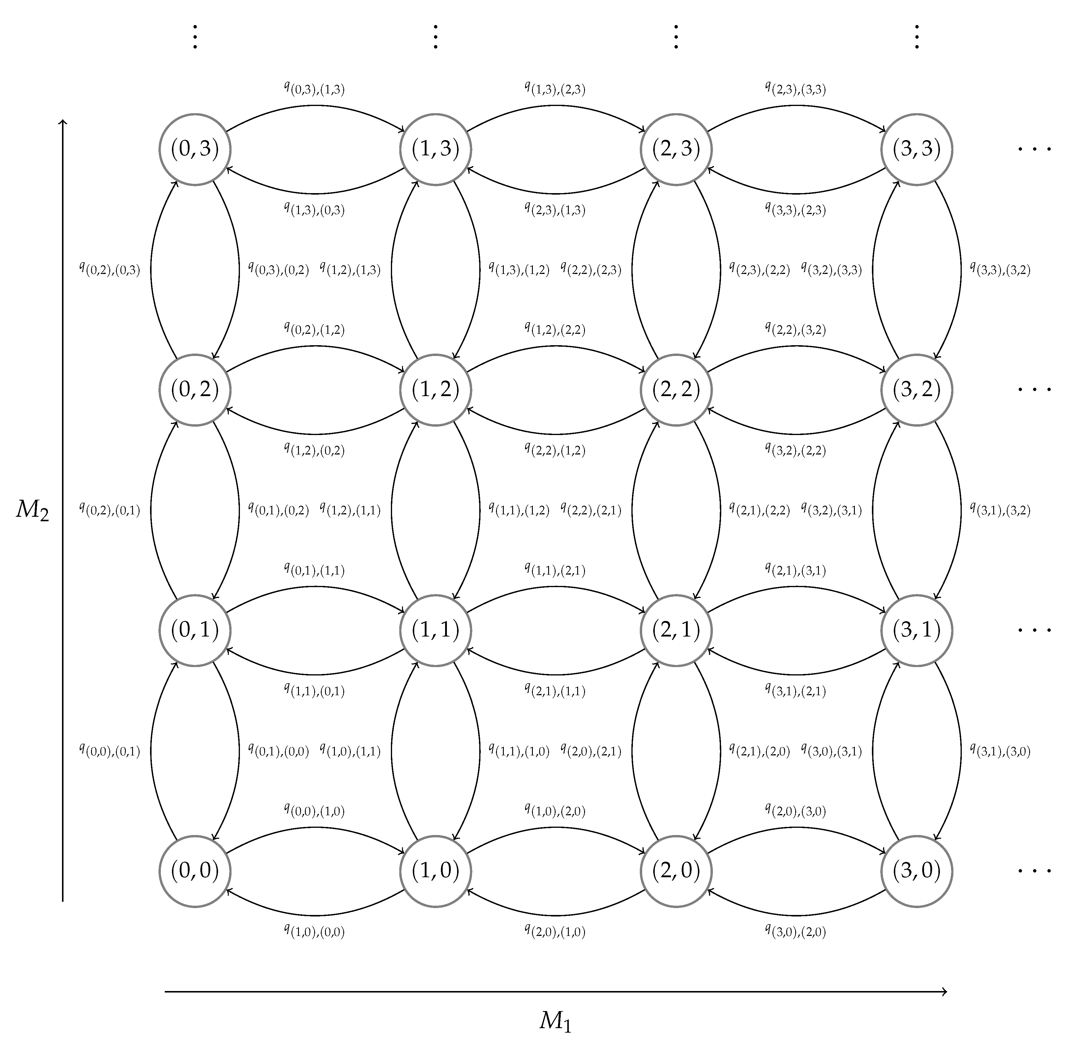
The dynamics of monomer formation and dissociation are then represented by jumps, or transitions, between states in S X , ( m 1 , m 2 ) ( m 1 , m 2 ) . The transition diagrams are shown in Figure 1b and Figure 2. We note that the boundaries of S X , which are not explicitly depicted in Figure 2, are determined by the conditions m 1 n R , 1 , m 2 n R , 2 and m 1 + m 2 n L . The infinitesimal transition rate from state ( m 1 , m 2 ) to state ( m 1 , m 2 ) , by assuming mass-action kinetics, is given by
q ( m 1 , m 2 ) , ( m 1 , m 2 ) = k f , 1 ( n R , 1 m 1 ) ( n L m 1 m 2 ) , if ( m 1 , m 2 ) = ( m 1 + 1 , m 2 ) , k r , 1 m 1 , if ( m 1 , m 2 ) = ( m 1 1 , m 2 ) , k f , 2 ( n R , 2 m 2 ) ( n L m 1 m 2 ) , if ( m 1 , m 2 ) = ( m 1 , m 2 + 1 ) , k r , 2 m 2 , if ( m 1 , m 2 ) = ( m 1 , m 2 1 ) , 0 , otherwise .
The process shown in Figure 2 is an example of a two-dimensional competition process, as introduced by Reuter [26] in 1961. In this type of process, jumps can be made from a given state to their nearest neighbours, as seen by the connecting arrows between states in Figure 2. Here we have two axes, each of which corresponds to a different receptor type, that is, the x-axis represents the number of type 1 monomers formed and the y-axis represents the number of type 2 monomers formed. In principle, as introduced by Iglehart [27] in his generalisation of Reuter’s work [26], one could add additional axes to represent further receptor variants competing for the same ligand; thus, expanding our model in Figure 1 to a multi-variate competition process (see the discussion in Section 5).
To illustrate the competition dynamics generated by the reactions in Figure 1a, we simulate in Figure 3 the stochastic model by means of the Gillespie algorithm [34]. We simulate the process for different numbers of molecules and K d values of the reactions, where K d , i = k r , i k f , i for i { 1 , 2 } . We vary these parameter values, as well as the number of available receptors of type 2, to see the effect on the competition dynamics. In all plots in Figure 3, n L = 10 2 , k r , 1 = k r , 2 = 10 3 s-1 and n R , 1 = 10 2 .
In the first plots of each row in Figure 3, we see that the process favours the formation of M 1 over M 2 . In this case, receptor type 1 out-competes receptor type 2 for ligand binding. In the second plot of each row, the number of molecules and rate constants governing the formation of M 1 and M 2 are identical and hence we see that the time courses for the two monomers are at a similar level, and are sometimes overlapping. Finally in the third plots of each row, we see that the receptors of type 2 are out-competing the receptors of type 1, and hence the time courses for M 2 are above those of M 1 . We also notice from Figure 3 that in some of the plots the process appears to reach a steady state by the end of the time course. One of the aims of this paper therefore, is to examine the effect of the rate constants and the number of molecules on the steady-state distribution of the process.
In Section 3 we compute two summary statistics of interest, namely the steady-state distribution of monomers on the cell surface [29,35] and the mean time to reach N monomers of one receptor type [29,36]. For each summary statistic, we present a computationally efficient matrix-analytic approach for its exact analysis, which can be implemented for low receptor and ligand numbers. Throughout this paper we will refer to this method of analysis as the exact matrix-analytic approach (EMA). Along with the exact analysis, and for scenarios where the large number of molecules leads to a huge number of states in S X , in turn making the EMA computationally intractable, we propose novel approximations to compute the proposed summary statistics. Finally, in Section 4 we compare the exact methods with the approximations, in order to quantify the goodness of the new approximations under different parameter regimes (i.e., in terms of the parameter values ( k f , 1 , k r , 1 , k f , 2 , k r , 2 ) of the model and the number of molecules).

3. Summary Statistics

3.1. Steady-State Distribution

In this section we analyse the steady-state distribution for the mathematical model defined in Section 2. We show how this distribution can be analytically computed by solving matrix equations in a computationally efficient way. Since this methodology is computationally limited by the number of molecules in the system, we propose as well approximations, which are based on the analysis of the process X when n L + or, equivalently, n L n R , 1 , n R , 2 . That is, instances when the competition for ligand is low. This analysis, when adjusting the number of available ligands to an effective number of ligands, leads to an approximation that can be used in low-to-moderate competition scenarios.

3.1.1. Exact Matrix-Analytic Approach (EMA)

The steady-state distribution for the model in Figure 1 is described in terms of the following probabilities
π ( m 1 , m 2 ) E M A = lim t + P { ( M 1 ( t ) , M 2 ( t ) ) = ( m 1 , m 2 ) } , ( m 1 , m 2 ) S X ,
which can be stored in a row vector π = ( π ( m 1 , m 2 ) , ( m 1 , m 2 ) S X ) for any given order of states in S X . These probabilities correspond to the number of monomers, of type 1 and type 2, respectively, found on the cellular surface at late times. They are known to satisfy [28] the system of equations
π · Q = 0 # S X , π · 1 # S X = 1 ,
where Q is the infinitesimal generator of the CTMC X , # S X is the number of states in the state space, 0 a is a row vector of zeros with length a and 1 a is a column vector of ones with length a.
The infinitesimal generator Q encodes the infinitesimal transition rates. Since the transitions described in Figure 2 only occur between adjacent states (see also Figure 1b), it is possible to order the states in S X so that Q is tri-diagonal by blocks, as shown in Appendix A. This means that the process X can be described as a level-dependent quasi-birth-and-death (LD-QBD) process [28]. For this type of process, efficient computational methods exist to solve Equation (2). In particular we use Algorithm A1, as presented in Appendix A, to compute the probabilities π ( m 1 , m 2 ) E M A for all ( m 1 , m 2 ) S X . Once these probabilities are in hand, one can compute the mean number of monomers at steady-state as
E E M A [ M 1 ] = m 1 = 0 N 1 m 1 m 2 = 0 m i n ( N 2 , n L m 1 ) π ( m 1 , m 2 ) E M A , E E M A [ M 2 ] = m 2 = 0 N 2 m 2 m 1 = 0 m i n ( N 1 , n L m 2 ) π ( m 1 , m 2 ) E M A ,
with N 1 = m i n ( n R , 1 , n L ) and N 2 = m i n ( n R , 2 , n L ) . However, as the number of molecules increases (see Appendix A), Algorithm A1 becomes computationally expensive, and an alternative approach needs to be considered.

3.1.2. No-Competition Approximation (NCA) under Excess of Ligand

We seek to find an approximation to the steady-state distribution which can be computationally tractable even for a large state space. To this aim, we note that as n L + (or, equivalently, n L n R , 1 , n R , 2 ), the two populations of monomers behave independently of one another given the excess of ligand. We therefore hypothesised that we could approximate the steady-state distribution in the large n L limit by considering two independent Markov chains for the variables M 1 ( t ) and M 2 ( t ) . In the limit n L + , given that the monomers are linked only by the number of ligands present, the steady-state probabilities for the two-dimensional process will be precisely equal to the product of the steady-state probabilities for the one-dimensional processes modelling M 1 ( t ) and M 2 ( t ) . This product, in the limit n L + , comprises what we denote by the no-competition approximation (NCA).
In particular, we define two independent Markov chains
X 1 = { M 1 ( t ) : t 0 } , X 2 = { M 2 ( t ) : t 0 } ,
for the monomers M 1 and M 2 , respectively, with state spaces
S X 1 = { m 1 N 0 = N { 0 } : m 1 N 1 } , S X 2 = { m 2 N 0 : m 2 N 2 } .
We note that, since the number of monomers in each CTMC can only increase or decrease by one unit in every transition (by means of monomer formation or dissociation), each CTMC X j , for  j { 1 , 2 } , is a birth-and-death process as depicted in Figure 4, with λ n = k f , j ( n R , j n ) ( n L n ) and μ n = k r , j n .
In the limit n L + , one can consider a constant number of ligands (not depleted by monomer formation); the binding rates then become λ n = k f , j n L ( n R , j n ) . For these rates, Equation (2) can be easily solved [25], as follows
π m 1 = lim t + P ( M 1 ( t ) = m 1 ) = n R , 1 m 1 k f , 1 n L k r , 1 + k f , 1 n L m 1 k r , 1 k r , 1 + k f , 1 n L n R , 1 m 1 , 0 m 1 N 1 ,
π m 2 = lim t + P ( M 2 ( t ) = m 2 ) = n R , 2 m 2 k f , 2 n L k r , 2 + k f , 2 n L m 2 k r , 2 k r , 2 + k f , 2 n L n R , 2 m 2 , 0 m 2 N 2 ,
which can be identified as binomial distributions. For these one-dimensional birth-and-death processes, X 1 and X 2 , one can determine the expected values of monomers in steady-state as
E N C A [ M 1 ] = m 1 = 0 N 1 m 1 π m 1 = k f , 1 n R , 1 n L k r , 1 + k f , 1 n L , E N C A [ M 2 ] = m 2 = 0 N 2 m 2 π m 2 = k f , 2 n R , 2 n L k r , 2 + k f , 2 n L .
In the limit n L + , the steady-state distribution of the process X is given by
π ( m 1 , m 2 ) N C A = π m 1 × π m 2 , ( m 1 , m 2 ) S X .
We note that, when n L + , one gets N 1 = n R , 1 , N 2 = n R , 2 and S X = { ( m 1 , m 2 ) N 0 2 : 0 m 1 N 1 , 0 m 2 N 2 } = S X 1 × S X 2 , so that Equations (4)–(7) are consistent.
It is clear that Equation (7) will also provide a reasonable approximation to the steady-state distribution when the number of ligands is much greater than the number of receptors, that is, n L n R , 1 , n R , 2 , since we are then in a situation in which there is very little competition between the receptors for available ligand, and hence, ligand depletion can be neglected, leading to two independent birth-and-death processes for the two different monomer populations. On the other hand, when n L is comparable in magnitude to n R , 1 + n R , 2 , Equation (7) overestimates the probabilities to reach higher numbers of monomers of each type, since it does not take into account the fact that ligands are being depleted by the formation of monomers in the competing Markov chain. To effectively approximate the steady-state distribution in scenarios where n L n R , 1 + n R , 2 , we propose to employ an effective number of ligands available to each birth-and-death process, n L * , which is lower than the total number of ligands in the two-dimensional process, n L . We propose that this effective number of ligands, and therefore an approximation to the steady-state distribution, can be reached iteratively using an algorithmic approach.

3.1.3. Moderate-Competition Approximation (MCA)

Here we propose Algorithm 1 to compute an approximate steady-state distribution, π ( m 1 , m 2 ) M C A , which can be used when n L n R , 1 + n R , 2 . In Algorithm 1, we iteratively reduce the total number of ligands available in each independent birth-and-death process X 1 and X 2 , by subtracting from n L the expected number of each monomer type in steady-state computed from the previous iteration. In each iteration i, the mean number of monomers in steady-state under the NCA approximation, E N C A , ( i ) [ M 1 ] and E N C A , ( i ) [ M 2 ] , are computed, and they are used to compute an effective number of free ligands available N L ( i + 1 ) , at iteration i + 1 . The iterative scheme stops once these mean values are close enough for two consecutive iterations, as determined by a threshold value ϵ . We note that the final number of ligands considered, n L * = N L ( i ) in the last iteration, can be seen as an effective number of ligands that reflects the competition for shared resources.
Algorithm 1 Iterative approximation for the steady-state distribution, ( π ( m 1 , m 2 ) M C A : ( m 1 , m 2 ) S X ) .
1:
i = 0 , N L ( i ) = n L ;
2:
Compute E N C A , ( i ) [ M 1 ] and E N C A , ( i ) [ M 2 ] from Equation (6), using N L ( i ) as the number of ligands in the system, instead of n L ;
3:
while E N C A , ( i ) [ M 1 ] E N C A , ( i 1 ) [ M 1 ] > ϵ or E N C A , ( i ) [ M 2 ] E N C A , ( i 1 ) [ M 2 ] > ϵ or i < 1 do:
4:
     i = i + 1 ;
5:
     N L ( i ) = ( n L E N C A , ( i 1 ) [ M 1 ] E N C A , ( i 1 ) [ M 1 ] ) α + N L ( i 1 ) ( 1 α ) ;
6:
    Compute E N C A , ( i ) [ M 1 ] and E N C A , ( i ) [ M 2 ] from Equation (6), using N L ( i ) instead of n L ;
7:
end while.
8:
Compute π m 1 N C A , ( i ) , for 0 m 1 N 1 , and π m 2 N C A , ( i ) , for 0 m 2 N 2 , from Equations (4)-(5)      using N L ( i ) instead of n L ;
9:
Compute π ( m 1 , m 2 ) M C A = π m 1 N C A , ( i ) × π m 2 N C A , ( i ) , ( m 1 , m 2 ) S X ;
10:
return π ( m 1 , m 2 ) M C A = π ( m 1 , m 2 ) M C A ( m 1 , m 2 ) S X π ( m 1 , m 2 ) M C A , ( m 1 , m 2 ) S X ; ▹ MCA steady-state distribution  
11:
return E M C A [ M 1 ] = m 1 = 0 N 1 m 1 m 2 = 0 m i n ( N 2 , n L m 1 ) π ( m 1 , m 2 ) M C A ; ▹ Mean number of type 1 monomers  
12:
return E M C A [ M 2 ] = m 2 = 0 N 2 m 2 m 1 = 0 m i n ( N 1 , n L m 2 ) π ( m 1 , m 2 ) M C A ; ▹ Mean number of type 2 monomers
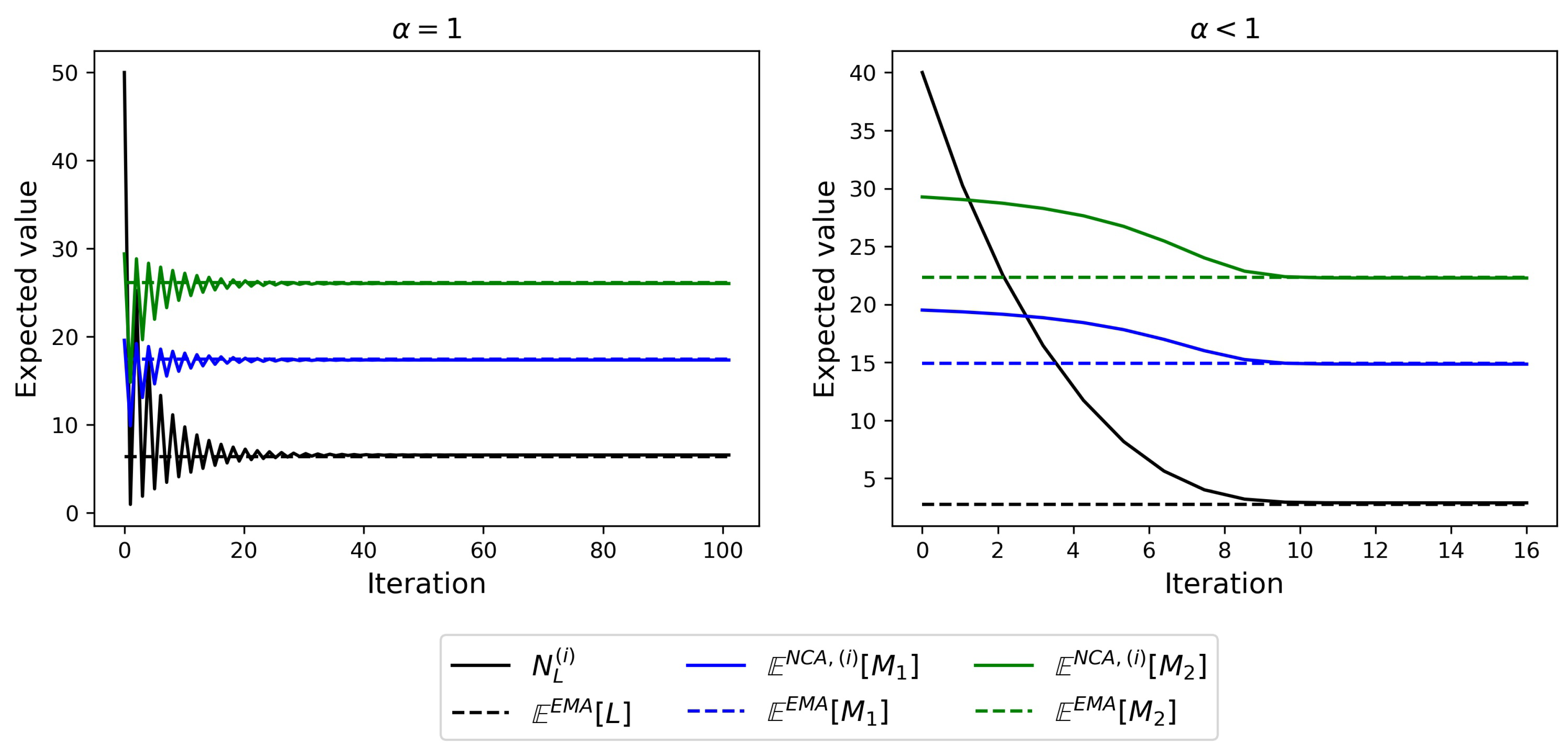
The parameter α ( α [ 0 , 1 ] ) is a tuning parameter needed in situations where n L < n R , 1 + n R , 2 . It modulates the convergence speed of the algorithm. We set α = 1 when n L n R , 1 + n R , 2 , since in this case it is impossible for n L E N C A , ( i 1 ) [ M 1 ] E N C A , ( i 1 ) [ M 1 ] to be negative at any iteration. Otherwise, when n L < n R , 1 + n R , 2 , the parameter α is chosen between 0 and 1 such that the effective number of ligands at every iteration in the algorithm is positive. Our numerical exploration indicates that the the choice of α does not affect the resulting steady-state probabilities π ( m 1 , m 2 ) M C A . When α = 1 , the expected number of monomers and ligands in steady-state exhibit damped oscillations as they converge. An example of this can be found on the left plot of Figure 5. When α < 1 , for values of α for which the algorithm converges, the expected number of monomers and ligands in steady-state either exhibit damped oscillations as they converge (for larger values of α ), or they decrease monotonically in convergence (for smaller values of α ). An example of monotonic convergence can be seen in the right plot of Figure 5. We found that for values of α for which there is monotonic convergence, the smaller the value of α , the more iterations the algorithm requires to converge. We note that in Figure 5, the mean number of free ligands in steady-state, as predicted by the EMA, is given by E E M A [ L ] = n L E E M A [ M 1 ] E E M A [ M 2 ] . Interestingly, we note how the values of N L ( i ) tend, in the limit i + , to this mean number of free ligands in steady-state.
In Section 4.1, we conduct a comprehensive numerical exploration of the accuracy of the MCA calculated with Algorithm 1 when compared to the exact steady-state distribution (EMA).

3.2. Timescales of Monomer Formation

In this section we study a second summary statistic of interest; namely the timescales of monomer formation. For the bi-variate process X , we define
T ( m 1 , m 2 ) ( N ) = i n f { t 0 : M 2 ( t ) = N | ( M 1 ( 0 ) , M 2 ( 0 ) ) = ( m 1 , m 2 ) } , ( m 1 , m 2 ) S X ,
to be the time to reach N monomers of type 2 (without loss of generality, since our arguments would similarly apply to type 1 monomers) given the initial state ( m 1 , m 2 ) S X . N can be any arbitrary value M 2 ( 0 ) < N N 2 , since T ( M 1 ( 0 ) , M 2 ( 0 ) ) ( M 2 ( 0 ) ) 0 .
Following the same strategy as that of Section 3.1, we first analyse T ( m 1 , m 2 ) ( N ) by means of an exact matrix-analytic approach. This implies solving a matrix equation for the two-dimensional process X described in Figure 2. This EMA is once again computationally limited by the number of molecules in the system. Thus, we analyse T ( m 1 , m 2 ) ( N ) in the limit as n L + (i.e., under effectively no competition for the shared ligand). We call this approximation the NCA. Based on this approximation, we propose the MCA, where an effective number of ligands is considered when computing this summary statistic.

3.2.1. Exact Matrix-Analytic Approach (EMA)

In this case, we can efficiently analyse T ( m 1 , m 2 ) ( N ) , for ( m 1 , m 2 ) S X with m 2 N , by means of first-step arguments. We omit the index N from now on to simplify our notation. One can, according to arguments described in Appendix B, compute the l-th order moment of T ( m 1 , m 2 ) , E T ( m 1 , m 2 ) l , by solving the system of linear equations:
Δ ( m 1 , m 2 ) E T ( m 1 , m 2 ) l = k f , 1 ( n R , 1 m 1 ) ( n L m 1 m 2 ) E T ( m 1 + 1 , m 2 ) l + k r , 1 m 1 E T ( m 1 1 , m 2 ) l + k f , 2 ( n R , 2 m 2 ) ( n L m 1 m 2 ) E T ( m 1 , m 2 + 1 ) l + k r , 2 m 2 E T ( m 1 , m 2 1 ) l + l E T ( m 1 , m 2 ) l 1 ,
with Δ ( m 1 , m 2 ) = k f , 1 ( n R , 1 m 1 ) ( n L m 1 m 2 ) + k r , 1 m 1 + k f , 2 ( n R , 2 m 2 ) ( n L m 1 m 2 ) + k r , 2 m 2 . This system of equations can be efficiently solved by arranging the states of the bi-variate Markov process X in levels L ( k ) , 0 k N 2 , as done for the steady-state distribution and detailed in Appendix A and Appendix B. We note that the system of equations given by Equation (8) can be solved in a iterative manner, for increasing values of l, where moments of order l can be computed once moments of order l 1 have been calculated (see Algorithm A2 in Appendix B). For l = 1 , we can then compute the mean time to reach N type 2 monomers, E E M A [ T ( m 1 , m 2 ) ( N ) ] , making use of the exact matrix-analytic methodology.

3.2.2. No-Competition Approximation (NCA) under Excess of Ligand

As an approximation under no competition ( n L + ), we can compute the mean time to reach N type 2 monomers by considering the independent one-dimensional birth-and-death process X 2 . In particular, we can analyse T m 2 ( N ) = i n f { t 0 : M 2 ( t ) = N | M 2 ( 0 ) = m 2 } for the process X 2 .
Let us focus on the mean value E [ T m 2 ( N ) ] for m 2 = 0 (that is, no type 2 monomers initially in the system), although we note that our arguments can be easily modified for different initial states 0 < m 2 < N , or for higher order moments of T m 2 ( N ) . It is clear that, for N = 1 , E [ T 0 ( 1 ) ] = 1 λ 0 . It is also clear from a first-step argument [25] that
E [ T i ( i + 1 ) ] = 1 λ i + μ i λ i E [ T i 1 ( i ) ] .
This allows one to recursively obtain
E [ T 0 ( N ) ] = 1 λ 0 + j = 1 N 1 μ 1 μ j λ 0 λ j i = 1 j λ 0 λ i 1 μ 1 μ i + 1 ,
which is similar to the well-known extinction time expressions for a one-dimensional birth-and-death process [25]. Thus, we propose the following approximation
E N C A [ T ( 0 , 0 ) ( N ) ] = 1 λ 0 + j = 1 N 1 μ 1 μ j λ 0 λ j i = 1 j λ 0 λ i 1 μ 1 μ i + 1 ,
when n L n R , 1 + n R , 2 .
In the case when n L is comparable to n R , 1 + n R , 2 , it is clear that E N C A [ T ( 0 , 0 ) ( N ) ] will underestimate the exact mean time to reach N type 2 monomers, E E M A [ T ( 0 , 0 ) ( N ) ] , since it does not take into account the ligands being depleted by the formation of monomers in the competing Markov chain. Thus, we propose next, an approximate method (MCA) to calculate E [ T ( 0 , 0 ) ( N ) ] , which can be used under low-to-moderate competition scenarios (i.e., when n L n R , 1 + n R , 2 ).

3.2.3. Moderate-Competition Approximation (MCA)

Since the NCA underestimates the time to reach N type 2 monomers, we now define the MCA, in order to approximately account for the depletion of ligand. In particular, we propose to compute E M C A [ T ( 0 , 0 ) ( N ) ] by implementing Equation (9), but with an effective number of free ligands
n L * = n L E [ M 1 ] ,
where E [ M 1 ] is the mean number of type 1 monomers in steady-state. We note here that, ideally, one would use E E M A [ M 1 ] in Equation (10). Alternatively, if this is computationally not feasible, one can use its approximation E M C A [ M 1 ] instead. From a practical perspective this does not seem crucial, since as we show in Section 4, E E M A [ M 1 ] and E M C A [ M 1 ] are almost equal (to integer value) in most of the scenarios considered.
We expect that the EMA will be approximated best by the NCA or the MCA depending on the number of molecules n R , 1 , n R , 2 and n L and the parameter values k f , 1 , k f , 2 , k r , 1 and k r , 2 . We explore the relationship between the EMA, NCA and MCA in terms of the parameters values and numbers of molecules in Section 4.2.

4. Results

In this section we analyse the behaviour of the different approximations described in Section 3 and compare them with the exact matrix-analytic approach. We do so numerically and for a wide range of parameter values and numbers of molecules, so as to identify regions of the parameter space for which the approximations are most accurate. In order to reduce the complexity of the numerical exploration we consider only the K d value for each reaction in Figure 1, where K d , i = k r , i / k f , i for i { 1 , 2 } , and not the individual forward and backward rate constants, by fixing k r , 1 = k r , 2 = 10 3  s−1 [6,37]. The value chosen for these rates is the common rate at which VEGFR1 and VEGFR2 dissociate their shared ligand, VEGF-A. The K d values and numbers of each receptor type are varied within the ranges given in Table 1, inspired from Reference [24] (Table 3), and which correspond to VEGFR1, VEGFR2 and VEGF-A. Finally, the number of ligands, n L , is varied to consider different competition regimes between the receptors, so that the comparisons between the EMA, NCA and MCA can be studied.

4.1. Steady-State Distribution

In this section we wish to compare the steady-state distributions computed via the EMA and the MCA, to determine how well the approximation works under different combinations of parameter values and number of molecules. We first present (see the first three columns of Figure 6) a comparison of the steady-state distributions computed via the EMA, NCA and MCA, for different numbers of ligands, n L , and where the number of receptors and other parameter values remain constant (see Table 1). In these heatmaps, the colour of each state indicates its steady-state probability. In the fourth and fifth columns, the colour represents the absolute difference | π ( m 1 , m 2 ) E M A π ( m 1 , m 2 ) N C A | or | π ( m 1 , m 2 ) E M A π ( m 1 , m 2 ) M C A | , respectively, for each state ( m 1 , m 2 ) S X . As the number of ligands, n L , decreases and becomes comparable to n R , 1 + n R , 2 , the NCA approximation worsens since the number of monomers of each type is overestimated. In contrast, we see that the MCA approximation remains similar to the EMA distribution, even for the lowest value of n L . It also better captures the mean number of monomers in steady-state than the NCA.
Having seen in Figure 6 that the MCA is able to accurately capture the steady-state distribution computed with the EMA for the specific number of molecules and parameter values chosen, we now seek to quantify the accuracy of the MCA for a wide range of parameter values and numbers of molecules. The Hellinger distance
H ( { π ( m 1 , m 2 ) E M A } ( m 1 , m 2 ) S X , { π ( m 1 , m 2 ) M C A } ( m 1 , m 2 ) S X ) 1 2 ( m 1 , m 2 ) S X π ( m 1 , m 2 ) E M A π ( m 1 , m 2 ) M C A 2 ,
is a way to measure the similarity between two discrete probability distributions. The Hellinger distance (HD) can take values between 0 and 1, where lower values indicate that the probability distributions are more similar.
Analysis of the Hellinger distances between the steady-state distributions can be found in Appendix C. Here, we focus on competing strength parameters. In particular, in Figure 7 we display scatter plots of the Hellinger distance as a function of the parameters n R , j / K d , j , j { 1 , 2 } . We note that the summary parameter n R , j / K d , j is an indicator of the competing strength of receptor type j, which will be large whenever there are many of these receptors in the system and/or they have high affinity for the common ligand. In Figure 7 we sample 10 3 parameter values ( K d , 1 , K d , 2 , n R , 1 , n R , 2 ) within the ranges of Table 1, from uniform distributions n R , j U ( 20 , 200 ) and K d , j = 10 x with x U ( 1 , 4 ) , for j { 1 , 2 } . We observe that the HD decreases with increasing n L , so that in the third plot where n L = 500 , the HD is relatively small, even for the largest sampled values of n R , 1 / K d , 1 and n R , 2 / K d , 2 . From the first plot in which n L = 10 2 , representing a high competition scenario, we observe larger values of the HD, especially when n R , 1 / K d , 1 and n R , 2 / K d , 2 are large. On the other hand, in the n L = 250 plot, smaller values of the competition strength parameters still lead to relatively small distances, indicating that even when n L is small comparable to n R , 1 + n R , 2 the approximation can still be reasonable if n R , 1 / K d , 1 and n R , 2 / K d , 2 are relatively small.
Although it is clear that there is some disparity between the probability distributions, especially when the competition is the highest, we note that the expected number of monomers in steady-state (not reported here) are almost identical between the two methods of computation. In particular, for all the sets ( K d , 1 , K d , 2 , n R , 1 , n R , 2 , n L ) of parameter values considered in Figure 7, the percentage error 100 · | 1 E E M A [ M j ] / E M C A [ M j ] | , j { 1 , 2 } , when computing the mean values through the MCA, instead of the EMA, is less than 5 % in all 10 3 cases. In fact, the overwhelming majority of parameter choices (991 out of 10 3 ) lead to the same mean values to integer precision, when choosing ϵ = 10 5 in Algorithm 1, even if the resulting Hellinger distance is relatively large.

4.2. Timescales of Monomer Formation

In this section we carry out a similar numerical exploration to that of Section 4.1, of the accuracy of the NCA and MCA for the expected time to reach N monomers of type 2. We note here that, while the NCA for the steady-state distribution can be seen as a necessary step to then propose the MCA in Algorithm 1, but where the MCA is always expected to behave better than the NCA, the NCA and the MCA can both lead to reasonable and complementary approximations to the EMA when studying the time to reach N type 2 monomers. Thus, our objective in this section is to compare the expected value of T ( 0 , 0 ) ( N ) derived via the EMA and the NCA/MCA. We plot in Figure 8 the mean time to reach N monomers, where N is represented as a percentage P of the steady-state number of monomers, N = P 100 E E M A [ M 2 ] , by means of the EMA, NCA and MCA. In low competition scenarios (e.g., large n L or when K d , 1 K d , 2 so that the dynamics of formation of type 1 monomers does not significantly affect the timescales of formation of type 2 monomers), the three approaches lead to almost indistinguishable results. For low-to-moderate competition settings, the MCA leads to a reasonable approximation. It is worth noting that the MCA and NCA seem to lead to lower and upper bounds for the mean time under analysis: the NCA always underestimates the timescales of type 2 monomer formation, by considering that there are n L ligands available, neglecting ligand depletion due to type 1 monomer formation competition; while the MCA tends to overestimate the timescales of type 2 monomer formation because one considers only n L E [ M 1 ] ligands available (that is, we remove from the beginning all the ligands occupied by steady-state type 1 monomers, even if these monomers may take some time to form). Since this steady-state amount of type 1 monomers takes some time to form, some of these ligands might still be able to contribute to the formation of type 2 monomers during early times, leading to the observed overestimation. Still, it is striking how well both approximations work when K d , 1 K d , 2 , even when the number of ligands is even less than the total number of receptors available in the system ( n L = 100 < 200 = n R , 1 + n R , 2 ).
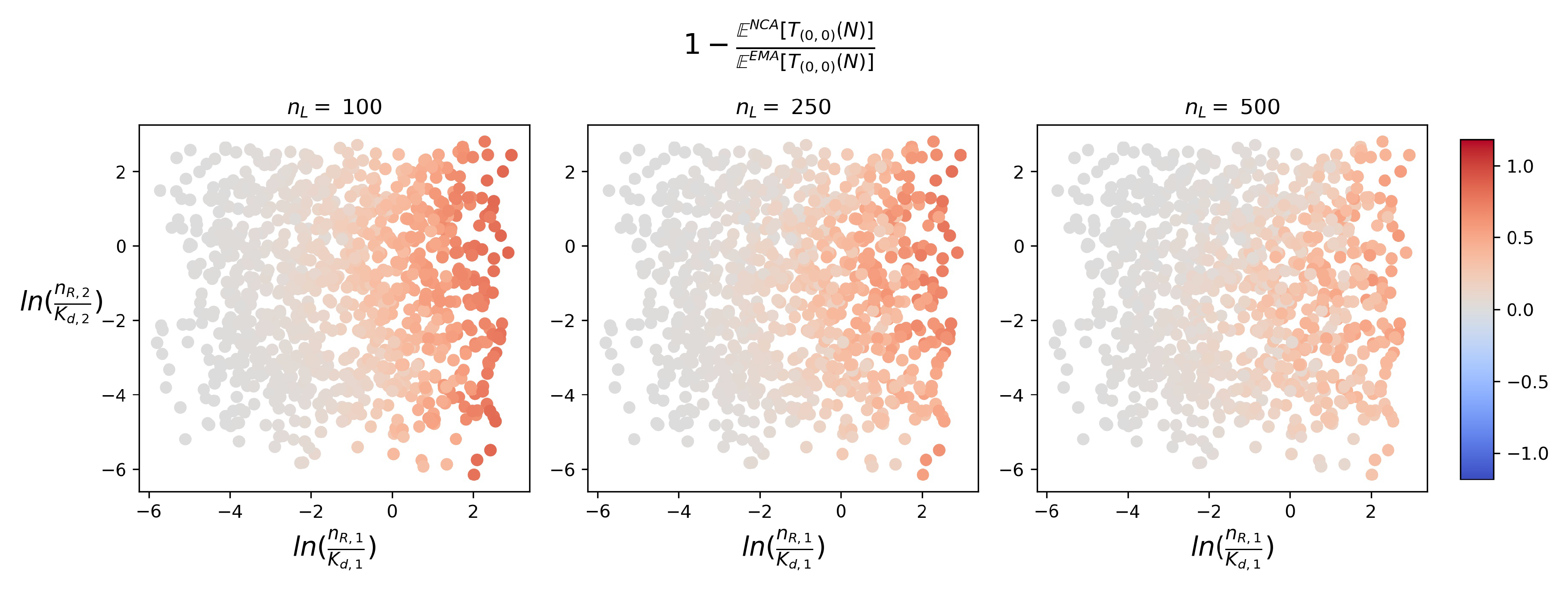
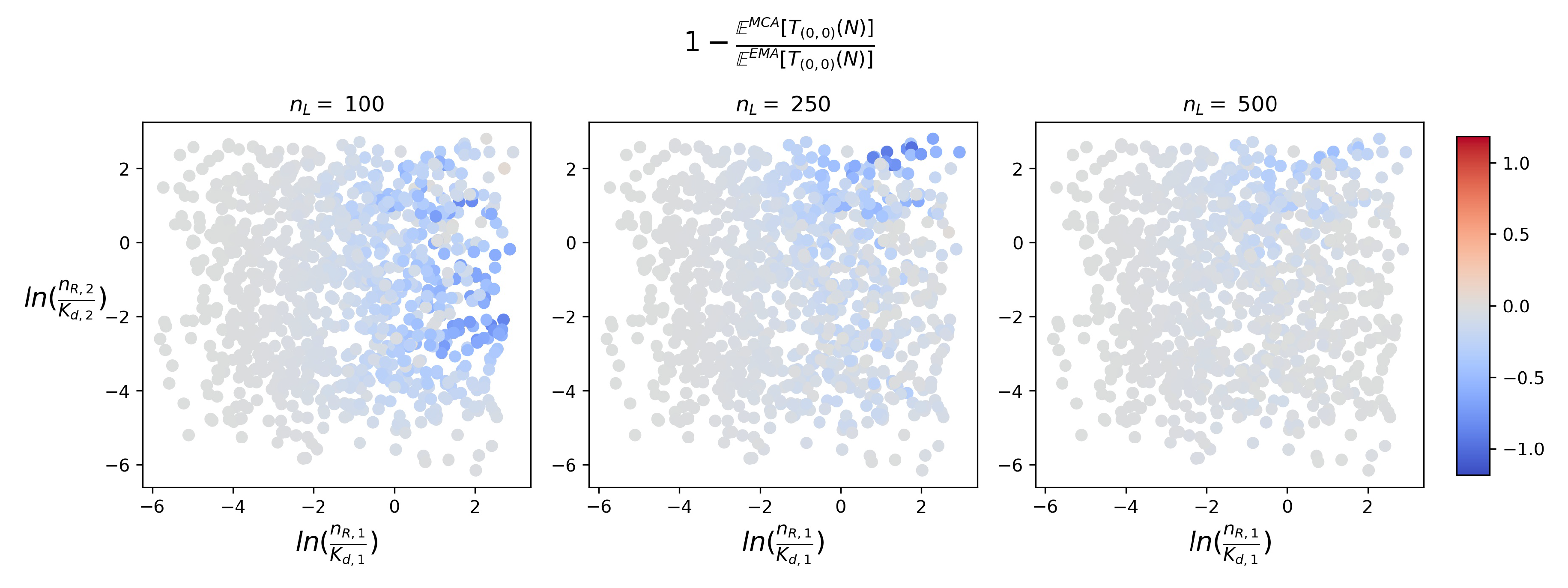
Analysis of the two approximations over a range of parameter values and number of molecules can be found in Appendix C. Here, and in order to better illustrate the effect of competition on the goodness of the NCA and MCA, we plot in Figure 9 and Figure 10 similar scatter plots to those of Figure 7, where we plot the relative differences between the mean times instead of the HD. From the first plot in Figure 9 we see that the relative difference increases with the competing strength parameter n R , 1 K d , 1 . However, similarly to the case of the steady-state distributions, as we increase n L , the competition from R 1 decreases and the NCA improves. For the sampled parameter sets, in general it seems that the MCA outperforms once again the NCA. Similarly to the NCA, the performance of the MCA tends to improve with large enough values of n L , where in the third plot of Figure 10 in which n L = 500 , more than half of the sampled parameter sets lead to an approximation with a relative error smaller than 5 % . It is clear that the MCA will behave rather well in situations where n L is large enough and, in particular, of a different order of magnitude to n R , 1 + n R , 2 ; for example, for n L = 2000 (data not shown here; note that n R , 1 + n R , 2 ranges from 40 to 400), an overwhelming majority of scenarios (more than 90 % ) in Figure 10 lead to MCA predictions with relative errors smaller than 5 % . Encouragingly also, we see that in Figure 9, all of the sampled points have relative differences greater than 0, which implies that the NCA always underestimates the EMA. This is expected given that the formation of monomers of type 2 will happen faster if there is no competition from another receptor, as assumed in the NCA. A similar pattern can be seen in Figure 10, in which the MCA tends to overestimate the EMA, leading to negative values of the relative difference. This is true for the majority of the points sampled. However, it is not always true as 6 of the 10 3 points sampled lead to very slightly positive relative differences (for  n L = 100 and n L = 250 only).
We finally note that the NCA may behave better than the MCA in situations where the mean steady-state number of type 1 monomers is perhaps non-negligible, but the timescales of type 1 monomer formation are significantly slower than the timescales of type 2 monomer formation. In these situations, considering an effective number of ligands n L E [ M 1 ] in Equation (10) might lead to worse predictions, since this ligand depletion might take very long to occur, and should, thus, be neglected, so that the NCA would prevail. An example of this behaviour can be seen in the left plot of Figure A3 in Appendix C.

4.3. Time to Signal Initiation: Reaching a Threshold Number of Productive Monomers

We illustrate an extension of our methodology by considering a stochastic descriptor that is linked to signal initiation for some receptor tyrosine kinases (RTKs)—the time to reach a threshold number N of productive monomers on the cell surface. In References [19,20], the authors hypothesise that signal initiation of T cells through the T cell receptor (TCR) is determined by the time a threshold number, N, of productive monomers is reached. A productive monomer is considered to be a receptor that remains bound to the ligand, for at least a dwell time τ . In References [19,20] the authors compute the mean time, T ( N , τ ) to reach N productive monomers. Note that T ( 0 , 0 ) ( N ) represents the time to reach a threshold number N of simultaneously bound monomers in the system, while T ( N , τ ) does not require these events to be simultaneous, but instead requires the corresponding monomers to be productive, based on the hypothesis that “counting devices are at work to allow signal accumulation, decoding and translation into biological responses”, as expressed in Reference [19].
The model in Figure 1a is proposed in Reference [19] when analysing T ( N , τ ) with a single receptor type (the TCR). Under ligand excess, authors in Reference [19] propose the approximation:
T ( N , τ ) = τ + 1 k f n L N n R + 1 2 ! N n R 2 + ,
where k f is the forward binding rate of the receptor, n R is the number of receptors available in the system, and N = e x p ( k r τ ) N represents the average number of binding events required for N productive ones to be reached. Recall that dissociation of a monomer occurs after an exponentially-distributed random time E x p ( k r ) , where k r is the dissociation rate of the receptor.
The authors in Reference [19] make use of experimental data to test two different hypotheses: that (a) the timescale of a T cell response correlates with the time it takes to have had N receptor-ligand complexes bound for at least a threshold dwell time, τ , each; or that (b) the timescale of a T cell response correlates with the time a threshold number, N, of TCRs must be occupied at equilibrium. Their conclusion is that experimental data supports hypotheses (a), but not (b). The descriptor T ( N , τ ) has been proposed in References [19,20] for the T cell receptor, and a similar hypothesis has been considered for other RTKs [18,29]. We make use of the methods introduced in previous sections, to compute T ( N , τ ) for a model as described in Figure 1a, where the receptor of interest for signal initiation (receptor 1) has a competitor (receptor 2) for binding the ligand.
We note that, by following similar arguments to those above, the NCA approximation for T ( N , τ ) consists of applying Equation (12) with the total number of ligands in the system n L , thus neglecting competition from receptor 2. On the other hand, as described in the MCA approximation, we may use Equation (12) with n L replaced by the effective number of ligands n L * = n L E [ M 2 ] .
Figure 11 shows a comparison between the mean time T ( N , τ ) , computed making use of the NCA and MCA approximations, and numerical simulations ( T S I M ( N , τ ) ). The matrix-analytic approach for this descriptor is not applicable since τ is fixed. We note that the time T ( N , τ ) to reach N productive type 1 monomers is not well estimated by the NCA (using Equation (12) with n L ligands) in situations where n L is not large enough (e.g., n L = 100 in Figure 11). The worst estimates are obtained in scenarios where the competing strength of receptor 1 is low, and that of receptor 2 is high, as one would expect. On the other hand, the MCA approach, using an effective number of ligands n L * , is better, even for a small number of ligands. In general, we observe that the MCA approximation gives good estimates of T ( N , τ ) over a wide range of parameter values: N and τ .

5. Discussion

In this paper, our focus has been on the modelling of receptor competition for a shared ligand. We have expressed this process as a multi-variate (bi-variate, in this case) competition process, as defined by Reuter [26] and Iglehart [27] in the area of Mathematical Ecology. We have shown how this leads to the study of a bi-dimensional structured continuous-time Markov chain; in particular, a level-dependent quasi-birth-and-death-process. For this process, our interest is in the analysis of two summary statistics related to late time (the steady-state distribution of monomers) and transient (the timescales of type 2 monomer formation, or of productive type 1 monomer formation) dynamics. For these summary statistics, it is possible to implement first-step arguments which lead to the study of systems of linear equations, where the number of equations is equal to (for the steady-state distribution), or potentially less than (for the timescales of monomer formation), the number of states in the CTMC, # S X . Since we are dealing with a LD-QBD process, there are matrix-oriented algorithms available in the literature [28], which we have exploited, that allow one to efficiently solve these systems.
The main limitation of this matrix-oriented approach is that the number of equations increases with the number of states, which turns out to increase with the number of molecules in the system, typically large in in vivo and in vitro settings [24]. Thus, we have proposed several approximations based on the analysis of the process in low-to-moderate competition scenarios (e.g., when the number of competing receptors is small, there is excess of ligand, or the competing receptor has a relatively low affinity compared to the other receptor). These approximations lead to the analysis of independent one-dimensional birth-and-death processes, for which analogous computations can be carried out much more efficiently. Our numerical results suggest that these approximations could be exploited in a wide range of parameter regimes, which have been explored inspired from values corresponding to the VEGF1 and VEGF2 receptors, which can bind the shared ligand, VEGF-A.
A striking advantage of using our approximate methods to compute the stochastic descriptors presented here is that the computational cost is much less than the cost of computing the same descriptors in an exact fashion (EMA). In Appendix D, Figure A4 and Figure A5, we present heatmaps of the central processing unit (CPU) times to run each method for both descriptors and a range of the numbers of molecules, n R , 1 and n R , 2 . From this analysis we find that, for the maximal values of n R , 1 and n R , 2 considered, the EMA takes over 40 min to compute the steady-state distribution, whereas the NCA and MCA can compute the distribution in a matter of seconds. Similarly, the EMA takes over 25 min to compute the mean time to reach N = n R , 2 2 monomers of type 2 for the maximal values of n R , 1 and n R , 2 considered, whereas the NCA and MCA again only take a few seconds. We note that as well as the CPU times, the EMA for both descriptors requires a large amount of memory for large values of n R , 1 and n R , 2 , whereas for the NCA and MCA the memory required is minimal. Results in Figure A4 and Figure A5 (see Appendix D) suggest that, due to both computational memory and time constrains, the MCA and NCA would allow us to analyse the summary statistics of interest in this system when dealing with numbers of molecules significantly beyond those that can be considered when implementing matrix-analytic approaches.
In this paper we have considered a system of two receptors which share a common ligand. We note, however, that the modelling framework, and the analytic and approximate methods of analysis of the summary statistics, could be extended and applied to any other system in which two species compete for a shared resource. For example, our model here could be reversed to represent two ligand molecules competing for a shared receptor, such as the competition by several ligands for the epidermal growth factor receptor (EGFR) (see Roepstorff et al. [38]). For example, two major ligands for the EGFR are the epidermal growth factor (EGF) and transforming growth factor α (TGF- α ). There are many other examples of multiple ligands stimulating the same receptor system to which our methodology could be applied [4,39,40]. Moreover, since our methods have been framed within processes originally devised in Mathematical Ecology, it is to be expected that they could be extended to more general competition processes in this area [41,42,43], not restricted to molecular dynamics.
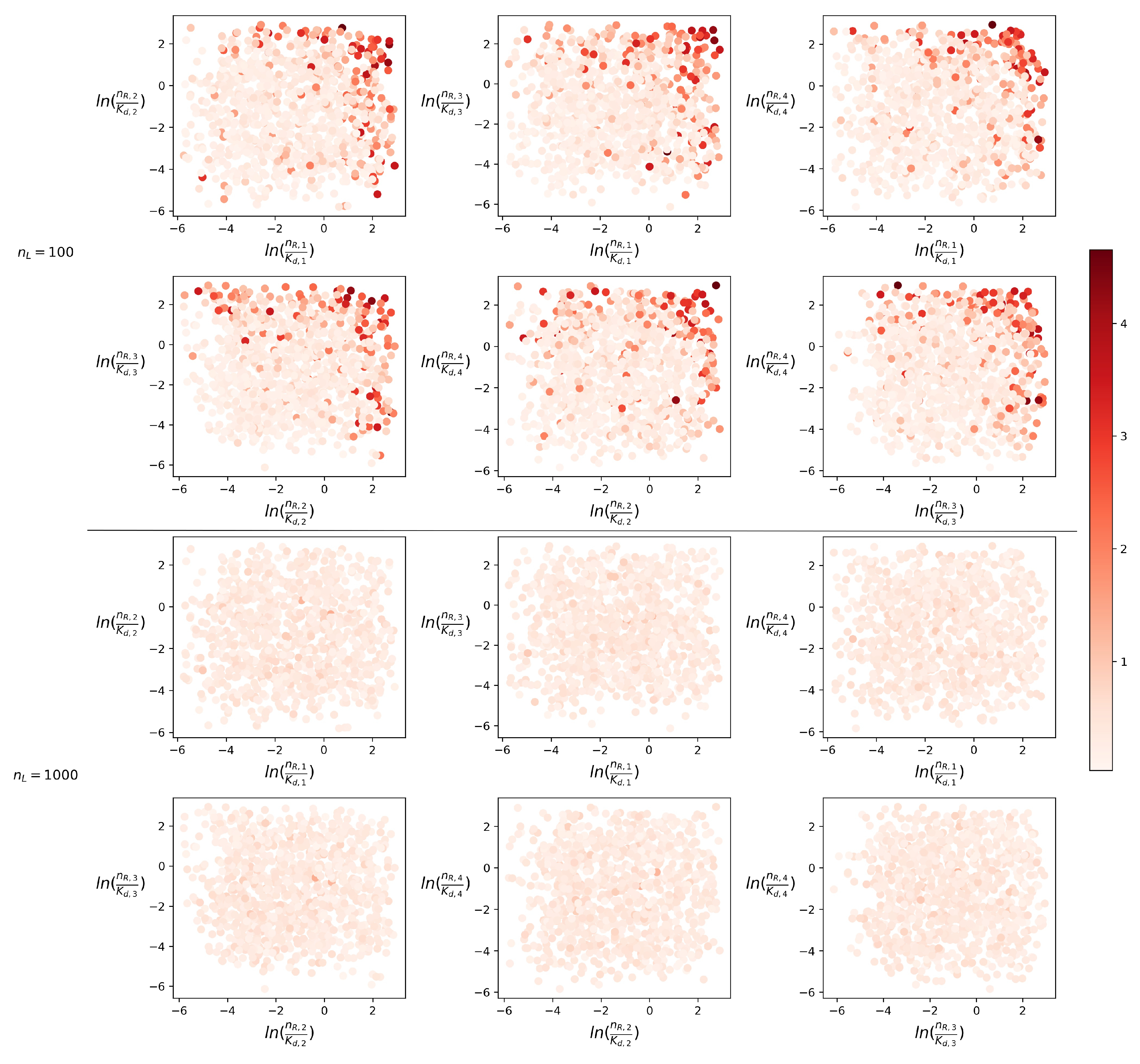
Similarly, although our methods have been presented for bi-variate processes, they could in principle be extended to higher dimensions, where the competition of M species for a shared resource (a structured M-dimensional continuous-time Markov chain) could be approximated as M independent birth-and-death processes, or as a different combination of lower-dimensional LD-QBDs if some competing sub-groups of species need to be analysed jointly. This can be especially useful since, while the systems of equations we are dealing with in the original bi-variate process are, when  n R , 1 + n R , 2 n L , of size ( n R , 1 + 1 ) · ( n R , 2 + 1 ) (see Appendix A), they would be of size ( n R , 1 + 1 ) · ( n R , 2 + 1 ) ( n R , M + 1 ) for a system with M receptors, making the matrix-oriented approach not feasible in practice. On the other hand, our approximations would be dealing instead with M independent birth-and-death processes, each of them of size n R , j + 1 , j { 1 , , M } . To illustrate the applicability of our approach in these higher-dimensional processes, we consider a situation with four different receptors competing for a common ligand. We plot in Figure 12 the absolute difference between the mean number of monomers in steady-state computed via the MCA and the mean number computed via stochastic simulations, for a wide range of parameter values, thus characterising different competition strengths for each receptor. We note that for the parameter regimes considered here (e.g., number of receptors ranging up to 2 × 10 2 for each species), the matrix-analytic approach is clearly unfeasible since it would require the analysis of CTMCs with more than 10 9 states. Thus, our NCA and MCA approximations allow one to analyse several descriptors of interest without having to implement these, numerically expensive, analytical methods. In particular, Figure 12 shows that the MCA approximation is able to capture, with high accuracy, these mean values of interest even for a small number of ligands (i.e., potentially high competition scenarios), unless the competing strengths of several receptors are too large. Even in these large competition scenarios, the MCA approach is able to estimate well these mean quantities for moderate ligand numbers (e.g., n L = 10 3 in Figure 12).
Finally, a clear limitation of our approach is that it has focused on receptor-ligand binding dynamics without taking into account additional reactions such as receptor synthesis, degradation or internalisation. Our analysis can be generalised to include those scenarios; for example, when modelling the surface and intra-cellular dynamics of two kinds of receptor competing (on the surface) for a common ligand, one could use our techniques to disentangle this competition, by the consideration of an effective number of ligands, so that the two intra-cellular processes can be separately studied. In the same way, our methodology has the potential to be of use in other settings. For example, since links between Queuing Theory and receptor-ligand interactions have been already established [44,45] (e.g., the two receptors in our system can be considered as two types of customers, waiting to be served by the common ligand (i.e., server)), one could explore the applicability of our NCA and MCA approximations to Queueing Systems (e.g., by modelling a multidimensional M/M/c system with k different types of arrivals being served by c common servers, as k independent M/M/c systems with an effective number of servers c * ). This is out of the scope of this manuscript and remains an area for future work.

Author Contributions

Conceptualization, P.-A.J., M.L.-G., M.C., G.L. and C.M.-P.; Data curation, P.-A.J.; Formal analysis, P.-A.J., M.L.-G. and M.C.; Funding acquisition, C.M.-P.; Investigation, P.-A.J. and M.L.-G.; Methodology, P.-A.J., M.L.-G. and M.C.; Software, P.-A.J.; Supervision, M.L.-G., G.L. and C.M.-P.; Visualization, P.-A.J.; Writing—Original draft, P.-A.J. and M.L.-G.; Writing—Review & editing, P.-A.J., M.L.-G., M.C., G.L. and C.M.-P. All authors have read and agreed to the published version of the manuscript.

Funding

PJ is supported by the EPSRC, AstraZeneca and Smith Institute (Smith Institute CASE studentship, award reference 1969354). MC is partially supported by grants FIS2016-78883-C2-2-P and PID2019-106339GB-I00 (Ministerio de Economía, Industria y Competitividad - Agencia Estatal de Investigación).

Acknowledgments

Numerical work was undertaken on ARC3, which is part of the High Performance Computing facilities at the University of Leeds, UK. We acknowledge and are grateful to the International Centre for Mathematical Sciences (ICMS), Edinburgh, where early discussions of this work took place during a Research in Groups programme (MLG, MC, GL and CMP).

Conflicts of Interest

The authors declare no conflict of interest.

Data Availability

Python (version 3.7) codes for computing the steady-state distribution and expected times to reach N monomers of type 2, via the EMA, NCA and MCA can be found in the public repository, “https://github.com/PollyJeffrey/Competition-modelling-paper”.

Abbreviations

   The following abbreviations are used in this manuscript:
EMAExact matrix-analytic approach
NCANo-competition approximation
MCAModerate-competition approximation

Appendix A

In this appendix we explain how the tri-diagonal by blocks structure of the infinitesimal generator matrix Q in Section 3 results from a particular ordering of the states in S X . We note first that the number of states in S X is
# S X = k = 0 N 2 ( m i n ( N 1 , n L k ) + 1 ) ,
where N 1 = m i n ( n R , 1 , n L ) and N 2 = m i n ( n R , 2 , n L ) . In fact, it is possible to obtain explicit formulae for the number of states in S X depending on the values of n R , 1 , n R , 2 and n L , as
# S X = ( n R , 1 + 1 ) ( n R , 2 + 1 ) , if n R , 1 + n R , 2 n L , ( n L n R , 1 + 1 ) ( n R , 1 + 1 ) + ( n R , 1 + n R , 2 n L ) ( n R , 1 + n L n R , 2 + 1 ) 2 , if n R , 1 n R , 2 n L and n R , 1 + n R , 2 > n L , ( n L n R , 2 + 1 ) ( n R , 2 + 1 ) + ( n R , 1 + n R , 2 n L ) ( n R , 2 + n L n R , 1 + 1 ) 2 , if n R , 2 n R , 1 n L and n R , 1 + n R , 2 > n L , ( n R , 2 + 1 ) ( 2 n L n R , 2 + 2 ) 2 , if n R , 1 > n L and n R , 2 < n L , ( n R , 1 + 1 ) ( 2 n L n R , 1 + 2 ) 2 , if n R , 1 < n L and n R , 2 > n L , ( n L + 1 ) ( n L + 2 ) 2 , if n R , 1 n L and n R , 2 n L .
This state space can be organised into levels, as follows,
S X = k = 0 N 2 L ( k ) , L ( k ) = { ( m 1 , m 2 ) S X : m 2 = k } , 0 k N 2 .
Thus, level L ( k ) = { ( 0 , k ) , ( 1 , k ) , . . . , ( m i n ( N 1 , n L k ) , k ) } contains those states representing k type 2 monomers present on the cell surface at any given time. If, when constructing the matrix Q , one orders the states by levels with L ( 0 ) L ( 1 ) . . . L ( N 2 ) , and states within each level L ( k ) as ( 0 , k ) ( 1 , k ) ( m i n ( N 1 , n L k ) , k ) , this leads to a tri-diagonal by blocks infinitesimal generator. In particular, from the transition diagram in Figure 2, it is clear that only transitions between adjacent states are allowed. This means that from any state ( m 1 , m 2 ) L ( m 2 ) , the next event in the Markov chain can take the process to either another state in level L ( m 2 ) , a state in level L ( m 2 + 1 ) , or a state in level L ( m 2 1 ) , by means of an association or dissociation reaction involving M 1 , an association to form M 2 or a dissociation of M 2 , respectively. Thus, since the process only moves up or down by a maximum of one level after each transition, the CTMC X is a level-dependent quasi-birth-and-death process (LD-QBD) [46], and the infinitesimal generator matrix Q is tri-diagonal by blocks. Q is given by
Q = Q 0 , 0 Q 0 , 1 0 0 0 Q 1 , 0 Q 1 , 1 Q 1 , 2 0 0 0 Q 2 , 1 Q 2 , 2 0 0 0 0 0 Q N 2 1 , N 2 1 Q N 2 1 , N 2 0 0 0 Q N 2 , N 2 1 Q N 2 , N 2 .
We note that each level L ( k ) contains J ( k ) = # L ( k ) = m i n ( N 1 , n L k ) + 1 states, so that each sub-matrix Q k , k has dimensions J ( k ) × J ( k ) . Sub-matrices Q k , k are given as follows:
  • For 1 k N 2 ,
    ( Q k , k 1 ) i , j = k r , 2 k , if j = i , 0 , otherwise ,
    for 0 i J ( k ) and 0 j J ( k 1 ) .
  • For 0 k N 2 1 ,
    ( Q k , k + 1 ) i , j = k f , 2 ( n R , 2 k ) ( n L i k ) , if j = i , 0 , otherwise ,
    for 0 i J ( k ) and 0 j J ( k + 1 ) .
  • For 0 k N 2 ,
    ( Q k , k ) i , j = k f , 1 ( n R , 1 i ) ( n L i k ) , if j = i + 1 , k r , 1 i , if j = i 1 , ( k f , 1 ( n R , 1 i ) ( n L i k ) + k r , 1 i + k f , 2 ( n R , 2 k ) ( n L i k ) + k r , 2 k ) , if j = i , 0 , otherwise ,
    for 0 i J ( k ) and 0 j J ( k ) .
This tri-diagonal by blocks form of the infinitesimal generator allows us to solve the steady-state matrix equations, Equation (2), with Algorithm A1, where π is comprised of row vectors π 0 , π 1 , , π N 2 which contain the ordered probabilities π ( m 1 , m 2 ) for the states in the corresponding level, π k = π ( 0 , k ) E M A , π ( 1 , k ) E M A , , π ( m i n ( N 1 , n L k ) , k ) E M A , 0 k N 2 . We note that Algorithm A1 is just an adapted version of the linear level reduction algorithm [47].
Algorithm A1 Computation of the steady-state distribution { π ( m 1 , m 2 ) E M A , ( m 1 , m 2 ) S X }  [47,48].
1:
H 0 = Q 0 , 0
2:
for k = 1 , , N 2 do
3:
     H k = Q k , k Q k , k 1 H k 1 1 Q k 1 , k
4:
end for
5:
Evaluate π N 2 * by solving π N 2 * H N 2 = 0 J ( N 2 ) with π N 2 * 1 J ( N 2 ) = 1
6:
for k = N 2 1 , , 0 do
7:
     π k * = π k + 1 * Q k + 1 , k H k 1
8:
end for
9:
for k = 0 , , N 2 do
10:
     π k = 1 k = 0 N 2 π k * 1 J ( k ) π k *
11:
end for
12:
return π = ( π 0 , , π N 2 ) ▹ EMA steady-state distribution

Appendix B

In this Appendix we present the details of the calculation of the moment of order l of the time to reach N monomers of type 2, starting from any initial state ( m 1 , m 2 ) , as introduced in Section 3. These moments can be obtained from the Laplace-Stieltjes transform of T ( m 1 , m 2 ) ( N ) , given by
ϕ ( m 1 , m 2 ) N ( z ) = E e z T ( m 1 , m 2 ) ( N ) , R ( z ) 0 .
The index N will be omitted from now on to simplify notation. Using a first-step argument, one finds the following system of linear equations
ϕ ( m 1 , m 2 ) ( z ) = k f , 1 ( n R , 1 m 1 ) ( n L m 1 m 2 ) z + Δ ( m 1 , m 2 ) ϕ ( m 1 + 1 , m 2 ) ( z ) + k r , 1 m 1 z + Δ ( m 1 , m 2 ) ϕ ( m 1 1 , m 2 ) ( z ) + k f , 2 ( n R , 2 m 2 ) ( n L m 1 m 2 ) z + Δ ( m 1 , m 2 ) ϕ ( m 1 , m 2 + 1 ) ( z ) k r , 2 m 2 z + Δ ( m 1 , m 2 ) ϕ ( m 1 , m 2 1 ) ( z ) ,
for ( m 1 , m 2 ) S X with m 2 < N , and where Δ ( m 1 , m 2 ) = k f , 1 ( n R , 1 m 1 ) ( n L m 1 m 2 ) + k r , 1 m 1 + k f , 2 ( n R , 2 m 2 ) ( n L m 1 m 2 ) + k r , 2 m 2 . Boundary conditions are given by ϕ ( m 1 , m 2 ) ( z ) 1 if m 2 = N , since T ( m 1 , m 2 ) ( m 2 ) 0 .
We note that E [ T ( m 1 , m 2 ) l ] = ( 1 ) l d l d z l ϕ ( m 1 , m 2 ) ( z ) z = 0 . Thus, once the Laplace-Stieltjes transforms are in hand, if we multiply Equation (A1) by ( 1 ) l , differentiate it with respect to zl times, and set z = 0 , we obtain the system of equations (8) for E T ( m 1 , m 2 ) l , for any l 1 .
Moreover, by arranging the states in S X in levels as in Appendix A, we note that each equation in the system (8) corresponds to an initial state ( m 1 , m 2 ) k = 0 N 1 L ( k ) , so that one can rewrite Equation (8) in matrix form as follows
m ( l ) = A m ( l ) + b ( l )
where
m ( l ) = m 0 ( l ) m 1 ( l ) m N 1 ( l ) , m k ( l ) = E [ T ( 0 , k ) l ] E [ T ( 1 , k ) l ] E [ T ( m i n ( N 1 , n L k ) , k ) l ] , 0 k N 1 .
Vector b ( l ) is also organised in sub-vectors as
b ( l ) = b 0 ( l ) b 1 ( l ) b N 1 ( l )
which are obtained from the ( l 1 ) t h order moments, as ( b k ( l ) ) ( m 1 , m 2 ) = l Δ ( m 1 , m 2 ) ( m k ( l 1 ) ) ( m 1 , m 2 ) , for all ( m 1 , m 2 ) L ( k ) ; we note that sub-vectors m k ( 0 ) are just column vectors of ones. Matrix A is given by
A = A 0 , 0 A 0 , 1 0 J ( 0 ) × J ( 2 ) 0 J ( 0 ) × J ( N 2 ) 0 J ( 0 ) × J ( N 1 ) A 1 , 0 A 1 , 1 A 1 , 2 0 J ( 1 ) × J ( N 2 ) 0 J ( 1 ) × J ( N 1 ) 0 J ( 2 ) × J ( 0 ) A 2 , 1 A 2 , 2 0 J ( 2 ) × J ( N 2 ) 0 J ( 2 ) × J ( N 1 ) 0 J ( N 2 ) × J ( 0 ) 0 J ( N 2 ) × J ( 1 ) 0 J ( N 2 ) × J ( 2 ) A N 2 , N 2 A N 2 , N 1 0 J ( N 1 ) × J ( 0 ) 0 J ( N 1 ) × J ( 1 ) 0 J ( N 1 ) × J ( 2 ) A N 1 , N 2 A N 1 , N 1 .
The sub-matrices A k , k are defined as follows:
  • For 1 k N 1 ,
    ( A k , k 1 ) i , j = k r , 2 k Δ ( i , k ) , if j = i , 0 , otherwise ,
    where 0 i J ( k ) and 0 j J ( k 1 ) .
  • For 0 k N 2 ,
    ( A k , k + 1 ) i , j = k f , 2 ( n R , 2 k ) ( n L i k ) Δ ( i , k ) , if j = i , 0 , otherwise ,
    where 0 i J ( k ) and 0 j J ( k + 1 ) .
  • For 0 k N 1 ,
    ( A k , k ) i , j = k f , 1 ( n R , 1 i ) ( n L i k ) Δ ( i , k ) , if j = i + 1 , k r , 1 i Δ ( i , k ) , if j = i 1 , 0 , otherwise ,
    where 0 i J ( k ) and 0 j J ( k ) .
Equation (A2) can then be solved efficiently using Algorithm A2 to obtain the l t h order moments of the random variable T ( m 1 , m 2 ) . In this algorithm, I a denotes the a × a identity matrix.
Algorithm A2 Moments of the random variable T ( m 1 , m 2 ) .
1:
( b k ( 1 ) ) ( m 1 , m 2 ) = 1 Δ ( m 1 , m 2 ) for all ( m 1 , m 2 ) L ( k ) , for k = 0 , , N 1
2:
R 0 = I J ( 0 ) A 0 , 0
3:
for p = 1 , , l do
4:
     S 0 = R 0 1 · b 0 ( p )
5:
    for k = 1 , N 1 do
6:
         R k = I J ( k ) A k , k A k , k 1 R k 1 1 A k 1 , k
7:
         S k = R k 1 A k , k 1 S k 1 + R k 1 b k ( p )
8:
    end for
9:
     m N 1 ( p ) = S N 1
10:
    for k = N 2 , , 0 do
11:
         m k ( p ) = S k + R k 1 A k , k + 1 m k + 1 ( p )
12:
    end for
13:
     ( b k ( p + 1 ) ) ( m 1 , m 2 ) = p + 1 Δ ( m 1 , m 2 ) ( m k ( p ) ) ( m 1 , m 2 ) , for all ( m 1 , m 2 ) L ( k ) , for k = 0 , , N 1
14:
end for
15:
return m ( l ) = ( m 0 T , , m N 1 T ) T l t h order moment of T ( m 1 , m 2 )

Appendix C

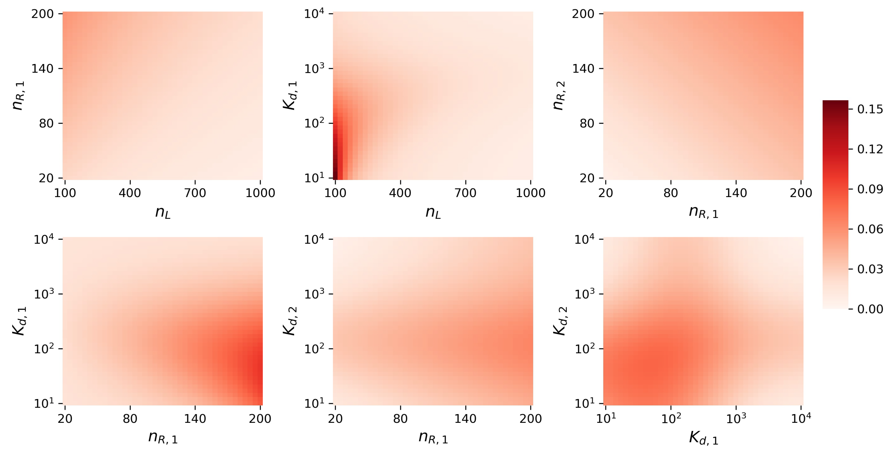
In this Appendix we analyse how similar the distributions { π ( m 1 , m 2 ) E M A } ( m 1 , m 2 ) S X and { π ( m 1 , m 2 ) M C A } ( m 1 , m 2 ) S X are for different parameter values ( K d , 1 , K d , 2 , n R , 1 , n R , 2 , n L ) , by plotting the corresponding Hellinger distance (HD) in Figure A1. The range of parameter values considered here allows us to consider scenarios of low to moderate and high competition between the two receptors for the shared ligand. The HD seems to be lower than 0.16 for all of the scenarios considered, even though in some of them, the number of ligands is significantly smaller than the total number of receptors (e.g., n L = 250 < 400 = 200 + 200 = n R , 1 + n R , 2 ). The number of molecules in the system does not, by itself, explain the goodness of the MCA; the dissociation constants K d , 1 and K d , 2 need also to be taken into account. Settings where both K d , 1 and K d , 2 are large (indicating the lowest affinity for ligand) correspond to low competition, since a small number of monomers of each type is formed, and then the baseline number of ligands considered, n L = 250 , is sufficient for the competition to be negligible. On the other hand, scenarios where for example, K d , 1 is small, can still lead to low competition if n L is sufficiently increased, or alternatively if n R , 1 decreased.
Figure A1. Hellinger distance between the steady-state distributions { π ( m 1 , m 2 ) E M A } ( m 1 , m 2 ) S X and { π ( m 1 , m 2 ) M C A } ( m 1 , m 2 ) S X . Baseline parameter values (that is, the value chosen in each plot for any parameter that has been fixed) are n R , 1 = 10 2 , n R , 2 = 10 2 , K d , 1 = 10 3 , K d , 2 = 10 3 and n L = 250 . We set the threshold parameter ϵ = 10 5 for the MCA.
Mathematics 08 01014 g0a1
When focusing on the time to reach N monomers of type 2, and similarly to the comprehensive sensitivity analysis carried out in Figure A1 for the steady-state distributions, we vary in Figure A2 the parameters ( K d , 1 , K d , 2 , n L , n R , 1 , n R , 2 ) in pairs, and plot heatmaps of the relative differences,
1 E N C A [ T ( 0 , 0 ) ( N ) ] E E M A [ T ( 0 , 0 ) ( N ) ] and 1 E M C A [ T ( 0 , 0 ) ( N ) ] E E M A [ T ( 0 , 0 ) ( N ) ] ,
for N = E E M A [ M 2 ] , so that T ( 0 , 0 ) ( N ) encodes the timescales for type 2 monomers to reach steady-state. We note that the MCA seems to better approximate the exact mean time in almost all parameter regimes explored in Figure A2. We expect however that the NCA might perform better in some scenarios (some of them can be identified in Figure A2), for example, when N is small (see Figure 8). Still, we observe in Figure A2 (left) that the NCA performs relatively well in parameter regimes representing low natural competition from R 1 , for example when K d , 1 is relatively large (indicative of low affinity of R 1 for L) and/or n R , 1 is small. In Figure A2 (right), this effect of competition from receptors of type 1 is reduced, and the MCA in general performs much better thanks to the effective ligand numbers considered in Equation (10), which takes into account ligand depletion due to receptor competition. We note that the MCA and the NCA lead to very similar, and almost exact, results under very low competition scenarios, since when E [ M 1 ] 0 , n L * n L in Equation (10) and thus, the two approximations are effectively the same.
Figure A2. Relative difference between the EMA and NCA (left) and MCA (right) expected times to reach N monomers of type 2. Baseline parameter values are n R , 1 = 10 2 , n R , 2 = 10 2 , K d , 1 = 10 3 , K d , 2 = 10 3 and n L = 250 .
Mathematics 08 01014 g0a2
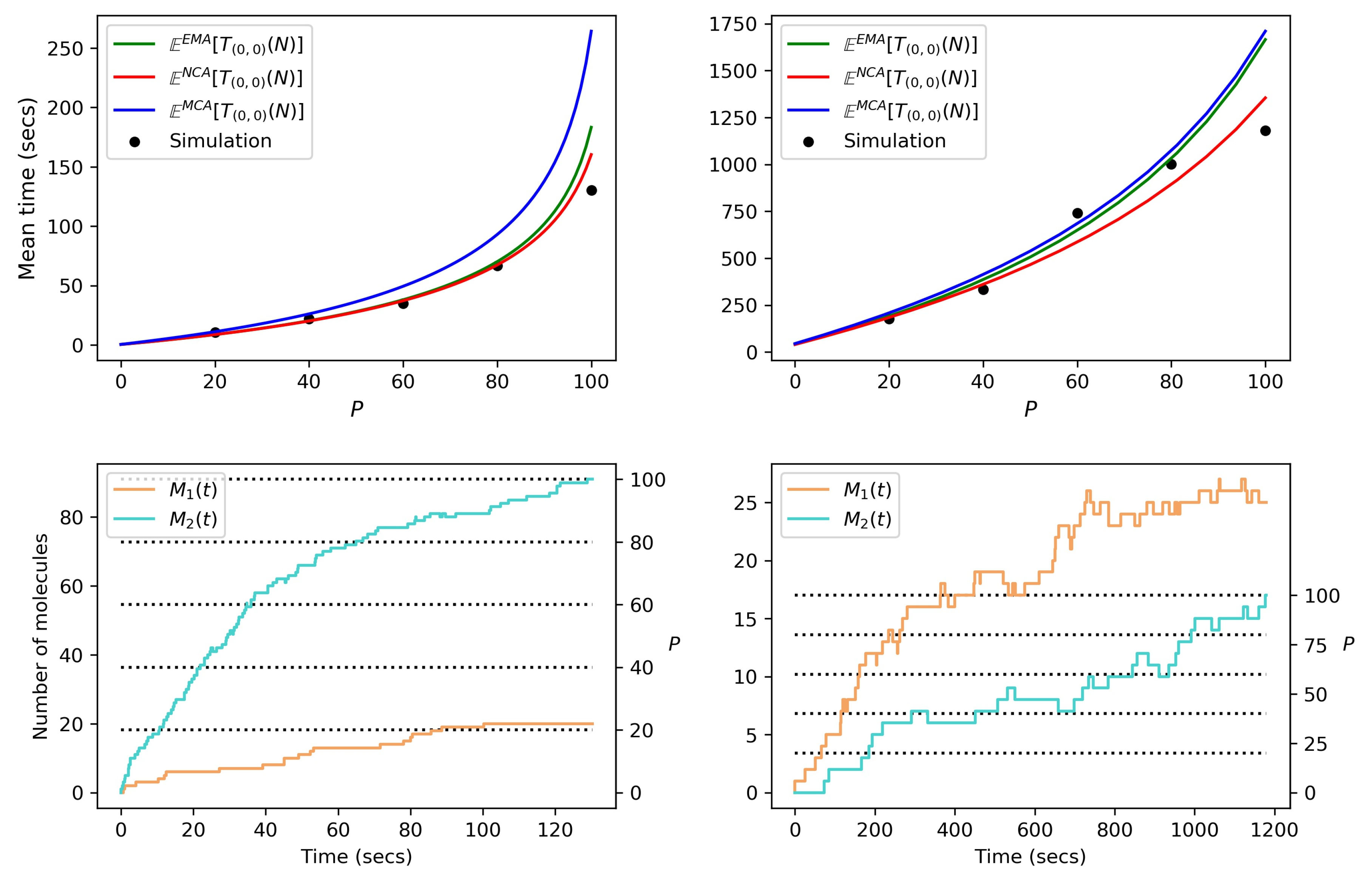
As mentioned in Section 4.2, there are some situations in which the NCA behaves better than the MCA. For example, the NCA seems to lead to better predictions than the MCA in Figure A3 (left), where the formation of type 2 monomers occurs more rapidly than that of type 1 monomers. In this figure, by carrying out a single stochastic (Gillespie) simulation of the process, we get a particular realisation of the time T ( 0 , 0 ) ( N ) to reach N = P 100 E E M A [ M 2 ] type 2 monomers, for different values of P; in particular, for P = 20 , 40, 60, 80 and 100 % of the average number of monomers in steady-state, we get the dots plotted in Figure A3 (top). On the other hand, in situations where the type 1 receptor is a strong competitor, such as in Figure A3 (right), the MCA outperforms the NCA.
Figure A3. Top: Comparison between the mean times computed using the EMA, NCA and MCA. P represents a percentage of the mean steady-state value, as in Figure 8, so that N = P 100 E E M A [ M 2 ] . Bottom: Stochastic realisations of the processes analysed in the top scenarios, leading to stochastic realisations (plotted as black dots in top plots) of random variable T ( 0 , 0 ) ( N ) for N = P 100 E E M A [ M 2 ] and different values of P. Left: n R , 1 = n R , 2 = 10 2 , K d , 1 = 10 2 and K d , 2 = 10 . Right: n R , 1 = 50 , n R , 2 = 10 2 , K d , 1 = 10 and K d , 2 = 10 3 . Number of ligands n L = 250 .
Mathematics 08 01014 g0a3

Appendix D

In this appendix we illustrate the computational advantage of using our approximations. In Figure A4 and Figure A5, a simple computational comparison between the NCA/MCA and the EMA is presented. In particular, we plot heatmaps of the central processing unit (CPU) times to run each method, for a range of numbers of the molecules n R , 1 and n R , 2 . In both figures, we set n L = 10,000 and K d , 1 = K d , 2 = 1000 . We note that, for a large number of ligands such as n L = 10,000, the computational cost of the EMA just depends on the values of n R , 1 and n R , 2 in Figure A4 and Figure A5 (see Appendix A, Algorithms A1 and A2), and is independent of K d , 1 and K d , 2 . The colour bar on each figure represents the CPU time for the computation of the summary statistic, with units minutes. We notice that, as expected, the EMA requires the largest amount of time to compute both descriptors since, especially when n R , 1 and n R , 2 are large, the method involves the computation of relatively large matrix inverses. There is a similar trend for both the NCA and MCA approaches to compute the steady-state distribution, that is, the larger n R , 1 and n R , 2 , the greater the CPU time. We see that, whereas the CPU time under the EMA takes up to a maximum of approximately 45 min, the NCA and MCA take less than 1 min for all numbers of molecules considered. For the second descriptor, we observe from Figure A5 that the EMA takes roughly half the CPU time as the EMA for the steady state distribution in Figure A4. This is since we are considering a value of N = n R , 2 2 , for the expected times and hence we are only inverting half the matrices as required in Figure A4. Again we see for the expected times in Figure A5, that the NCA and MCA are strikingly faster to compute than the EMA. As expected, the NCA in this case does not depend on the value of n R , 1 since this quantity does not feature in the calculation. For the MCA however, we must first compute E M C A [ M 1 ] using the MCA for the steady-state distribution and hence the CPU times here do depend on n R , 1 .
In Figure A6, we explore in more detail specific pixels from Figure A4 and Figure A5. In particular we choose 3 values of n R , 2 , corresponding to the 3 columns in Figure A6 and vary on the x-axis of each plot, the value of n R , 1 . We are thus considering in each plot of Figure A6, a cross-section of the heatmaps in Figure A4 and Figure A5. The top row of Figure A6 relates to the steady-state distribution descriptor and hence the y-axis of the plots in this row is the Hellinger distance. The second row in the figure relates to the expected times to reach N monomers of type 2 descriptor and hence the y-axis of the plots in this row is the relative difference as plotted in Figure 9 and Figure 10. Finally the colour bar represents the CPU time saved with units minutes, by computing the descriptors using the approximations (NCA and MCA) instead of the analytic (EMA). For the steady state descriptor in the first row we see that as expected the Hellinger distance between the EMA and the NCA increases as n R , 1 increases, whereas the Hellinger distance between the EMA and the MCA remains almost constant, indicating that this approximation works very well for these numbers of molecules. As we increase n R , 1 and n R , 2 we find that the time saved by using the NCA or MCA increases. In the second row we note that both the NCA and MCA worsen as approximations as we increase n R , 1 , but this worsening is only very slight (the relative differences are always 1 ). Again we see that as we increase n R , 1 and n R , 2 the time saved by using the NCA or MCA increases. From this figure we see that there is a “playoff” between the Hellinger distance or relative difference and the CPU time saved, but for the numbers of molecules and parameter values considered here, the time saved clearly outweighs the slight deviation from the EMA result caused by using the MCA for the steady state distribution and both the NCA and MCA for the expected times descriptor.
Figure A4. Comparison of CPU time (in minutes) required to compute the steady-state distribution for the EMA, NCA and MCA for different receptor numbers.
Mathematics 08 01014 g0a4
Figure A5. Comparison of CPU time (in minutes) required to compute the mean time to reach N = n R , 2 2 monomers of type 2 for the EMA, NCA and MCA for different receptor numbers.
Mathematics 08 01014 g0a5
Figure A6. Top: Playoff between the Hellinger distance, the value of n R , 1 and the CPU time saved by considering either the NCA or MCA instead of the EMA when computing the steady state distribution. Bottom: Playoff between the relative difference, the value of n R , 1 and the CPU time saved by considering either the NCA or MCA instead of the EMA when computing the expected time to reach N monomers of type 2. In all plots, n L = 10,000 and K d , 1 = K d , 2 = 1000 .
Mathematics 08 01014 g0a6

References

  1. Santos, S.D.; Verveer, P.J.; Bastiaens, P.I. Growth factor-induced MAPK network topology shapes Erk response determining PC-12 cell fate. Nat. Cell Biol. 2007, 9, 324. [Google Scholar] [CrossRef] [PubMed]
  2. Katoh, M.; Katoh, M. FGF signaling network in the gastrointestinal tract. Int. J. Oncol. 2006, 29, 163–168. [Google Scholar] [CrossRef] [PubMed] [Green Version]
  3. Ernst, M.; Jenkins, B.J. Acquiring signalling specificity from the cytokine receptor gp130. Trends Genet. 2004, 20, 23–32. [Google Scholar] [CrossRef] [PubMed]
  4. Chen, S.; Guo, X.; Imarenezor, O.; Imoukhuede, P. Quantification of VEGFRs, NRP1, and PDGFRs on endothelial cells and fibroblasts reveals serum, intra-family ligand, and cross-family ligand regulation. Cell. Mol. Bioeng. 2015, 8, 383–403. [Google Scholar] [CrossRef]
  5. Hackel, P.O.; Zwick, E.; Prenzel, N.; Ullrich, A. Epidermal growth factor receptors: critical mediators of multiple receptor pathways. Curr. Opin. Cell Biol. 1999, 11, 184–189. [Google Scholar] [CrossRef]
  6. Weddell, J.C.; Imoukhuede, P.I. Integrative meta-modeling identifies endocytic vesicles, late endosome and the nucleus as the cellular compartments primarily directing RTK signaling. Integr. Biol. 2017, 9, 464–484. [Google Scholar] [CrossRef] [Green Version]
  7. Riese, D.J.; Stern, D.F. Specificity within the EGF family/ErbB receptor family signaling network. Bioessays 1998, 20, 41–48. [Google Scholar] [CrossRef]
  8. López-García, M.; Nowicka, M.; Fearnley, G.W.; Ponnambalam, S.; Lythe, G.; Molina-París, C. Performance measures in stochastic processes and the matrix-analytic approach. In Quantitative Biology: Theory, Computational Methods, and Models; Springer: Cham, Switzerland, 2018; pp. 379–402. [Google Scholar]
  9. Starbuck, C.; Lauffenburger, D.A. Mathematical model for the effects of epidermal growth factor receptor trafficking dynamics on fibroblast proliferation responses. Biotechnol. Progress 1992, 8, 132–143. [Google Scholar] [CrossRef]
  10. Cross, M.J.; Dixelius, J.; Matsumoto, T.; Claesson-Welsh, L. VEGF-receptor signal transduction. Trends Biochem. Sci. 2003, 28, 488–494. [Google Scholar] [CrossRef]
  11. Shibuya, M. Differential roles of vascular endothelial growth factor receptor-1 and receptor-2 in angiogenesis. BMB Rep. 2006, 39, 469–478. [Google Scholar] [CrossRef]
  12. Dikov, M.M.; Ohm, J.E.; Ray, N.; Tchekneva, E.E.; Burlison, J.; Moghanaki, D.; Nadaf, S.; Carbone, D.P. Differential roles of vascular endothelial growth factor receptors 1 and 2 in dendritic cell differentiation. J. Immunol. 2005, 174, 215–222. [Google Scholar] [CrossRef] [PubMed] [Green Version]
  13. Kozer, N.; Barua, D.; Orchard, S.; Nice, E.C.; Burgess, A.W.; Hlavacek, W.S.; Clayton, A.H. Exploring higher-order EGFR oligomerisation and phosphorylation—A combined experimental and theoretical approach. Mol. bioSyst. 2013, 9, 1849–1863. [Google Scholar] [CrossRef] [PubMed] [Green Version]
  14. Lauffenburger, D.A.; Linderman, J.J. Receptors: Models for Binding, Trafficking, and Signaling; Oxford University Press on Demand: Oxford, UK, 1996. [Google Scholar]
  15. Waters, C.M.; Oberg, K.C.; Carpenter, G.; Overholser, K.A. Rate constants for binding, dissociation, and internalization of EGF: Effect of receptor occupancy and ligand concentration. Biochemistry 1990, 29, 3563–3569. [Google Scholar] [CrossRef] [PubMed]
  16. Klein, P.; Mattoon, D.; Lemmon, M.A.; Schlessinger, J. A structure-based model for ligand binding and dimerization of EGF receptors. Proc. Natl. Acad. Sci. USA 2004, 101, 929–934. [Google Scholar] [CrossRef] [Green Version]
  17. Blinov, M.L.; Faeder, J.R.; Goldstein, B.; Hlavacek, W.S. A network model of early events in epidermal growth factor receptor signaling that accounts for combinatorial complexity. Biosystems 2006, 83, 136–151. [Google Scholar] [CrossRef]
  18. Alarcón, T.; Page, K.M. Stochastic models of receptor oligomerization by bivalent ligand. J. R. Soc. Interface 2006, 3, 545–559. [Google Scholar] [CrossRef] [Green Version]
  19. Currie, J.; Castro, M.; Lythe, G.; Palmer, E.; Molina-París, C. A stochastic T cell response criterion. J. R. Soc. Interface 2012, 9, 2856–2870. [Google Scholar] [CrossRef] [Green Version]
  20. Castro, M.; van Santen, H.M.; Férez, M.; Alarcón, B.; Lythe, G.; Molina-París, C. Receptor pre-clustering and T cell responses: Insights into molecular mechanisms. Front. Immunol. 2014, 5, 132. [Google Scholar] [CrossRef] [Green Version]
  21. Bel, G.; Munsky, B.; Nemenman, I. The simplicity of completion time distributions for common complex biochemical processes. Phys. Biol. 2009, 7, 016003. [Google Scholar] [CrossRef] [Green Version]
  22. Resat, H.; Ewald, J.A.; Dixon, D.A.; Wiley, H.S. An integrated model of epidermal growth factor receptor trafficking and signal transduction. Biophys. J. 2003, 85, 730–743. [Google Scholar] [CrossRef] [Green Version]
  23. Gurevich, K.G.; Agutter, P.S.; Wheatley, D.N. Stochastic description of the ligand—Receptor interaction of biologically active substances at extremely low doses. Cell. Signal. 2003, 15, 447–453. [Google Scholar] [CrossRef]
  24. López-García, M.; Nowicka, M.; Bendtsen, C.; Lythe, G.; Ponnambalam, S.; Molina-Paris, C. Stochastic models of the binding kinetics of VEGF-A to VEGFR1 and VEGFR2 in endothelial cells. arXiv 2016, arXiv:1606.07269. [Google Scholar]
  25. Allen, L.J. An Introduction to Stochastic Processes with Applications to Biology; Chapman and Hall/CRC: Boca Raton, FL, USA, 2010. [Google Scholar]
  26. Reuter, G. Competition processes. In Proceedings of the 4th Berkeley Symposium Mathematcial Statistics and Probability, Berkeley, CA, USA, 20 June–30 July 1961; Volume 2, pp. 421–430. [Google Scholar]
  27. Iglehart, D.L. Multivariate competition processes. Ann. Math. Stat. 1964, 35, 350–361. [Google Scholar] [CrossRef]
  28. Latouche, G.; Ramaswami, V.; Kulkarni, V. Introduction to matrix analytic methods in stochastic modeling. J. Appl. Mathe. Stoch. Anal. 1999, 12, 435–436. [Google Scholar]
  29. López-García, M.; Nowicka, M.; Bendtsen, C.; Lythe, G.; Ponnambalam, S.; Molina-París, C. Quantifying the phosphorylation timescales of receptor–ligand complexes: A Markovian matrix-analytic approach. Open Biol. 2018, 8, 180126. [Google Scholar] [CrossRef] [Green Version]
  30. De la Higuera, L.; López-García, M.; Lythe, G.; Molina-París, C. IL-2 Stimulation of Regulatory T Cells: A Stochastic and Algorithmic Approach. In Modeling Cellular Systems; Springer: Cham, Switzerland, 2017; pp. 81–105. [Google Scholar]
  31. Economou, A.; Gómez-Corral, A.; López-García, M. A stochastic SIS epidemic model with heterogeneous contacts. Physica A Stat. Mech. Appl. 2015, 421, 78–97. [Google Scholar] [CrossRef] [Green Version]
  32. López-García, M. Stochastic descriptors in an SIR epidemic model for heterogeneous individuals in small networks. Math. Biosci. 2016, 271, 42–61. [Google Scholar] [CrossRef] [Green Version]
  33. Steinfeld, J.I.; Francisco, J.S.; Hase, W.L. Chemical Kinetics and Dynamics; Prentice Hall: Englewood Cliffs, NJ, USA, 1989; Volume 3. [Google Scholar]
  34. Gillespie, D.T. A general method for numerically simulating the stochastic time evolution of coupled chemical reactions. J. Comput. Phys. 1976, 22, 403–434. [Google Scholar] [CrossRef]
  35. Stroock, D.W. An Introduction to Markov Processes; Springer Science & Business Media: Berlin, Germany, 2013; Volume 230. [Google Scholar]
  36. Karlin, S. A First Course in Stochastic Processes; Academic Press: Cambridge, MA, USA, 2014. [Google Scholar]
  37. Weddell, J.C.; Imoukhuede, P. Quantitative characterization of cellular membrane-receptor heterogeneity through statistical and computational modeling. PLOS ONE 2014, 9, e97271. [Google Scholar] [CrossRef] [Green Version]
  38. Roepstorff, K.; Grandal, M.V.; Henriksen, L.; Knudsen, S.L.J.; Lerdrup, M.; Grøvdal, L.; Willumsen, B.M.; Van Deurs, B. Differential effects of EGFR ligands on endocytic sorting of the receptor. Traffic 2009, 10, 1115–1127. [Google Scholar] [CrossRef]
  39. Schmidt, A.M.; Du Yan, S.; Yan, S.F.; Stern, D.M. The biology of the receptor for advanced glycation end products and its ligands. Biochim. Biophys. Acta (BBA) Mol. Cell Res. 2000, 1498, 99–111. [Google Scholar] [CrossRef] [Green Version]
  40. Ma, B.; Shatsky, M.; Wolfson, H.J.; Nussinov, R. Multiple diverse ligands binding at a single protein site: A matter of pre-existing populations. Protein Sci. 2002, 11, 184–197. [Google Scholar] [CrossRef] [PubMed]
  41. Gómez-Corral, A.; López-García, M. Extinction times and size of the surviving species in a two-species competition process. J. Math. Biol. 2012, 64, 255–289. [Google Scholar] [CrossRef]
  42. Gómez-Corral, A.; López-García, M. On the number of births and deaths during an extinction cycle, and the survival of a certain individual in a competition process. Comput. Math. Appl. 2012, 64, 236–259. [Google Scholar] [CrossRef] [Green Version]
  43. Gómez-Corral, A.; López-García, M. Lifetime and reproduction of a marked individual in a two-species competition process. App. Math. Compu. 2015, 264, 223–245. [Google Scholar] [CrossRef] [Green Version]
  44. Wedagedera, J.R.; Burroughs, N.J. T-cell activation: A queuing theory analysis at low agonist density. Biophys. J. 2006, 91, 1604–1618. [Google Scholar] [CrossRef] [Green Version]
  45. Wedagedara, J. Some large deviation estimates for an Erlang queue of phosphorylated T-cell receptors. J. Natl. Sci. Found. Sri Lanka 2011, 39, 03–12. [Google Scholar] [CrossRef] [Green Version]
  46. Kulkarni, V.G. Modeling and Analysis of Stochastic Systems; Chapman and Hall/CRC: Boca Raton, FL, USA, 2016. [Google Scholar]
  47. Gaver, D.; Jacobs, P.; Latouche, G. Finite birth-and-death models in randomly changing environments. Adv. Appl. Probab. 1984, 16, 715–731. [Google Scholar] [CrossRef]
  48. Gómez-Corral, A.; López-García, M. Perturbation analysis in finite LD-QBD processes and applications to epidemic models. Numer. Linear Algebra Appl. 2018, 25, e2160. [Google Scholar] [CrossRef] [Green Version]
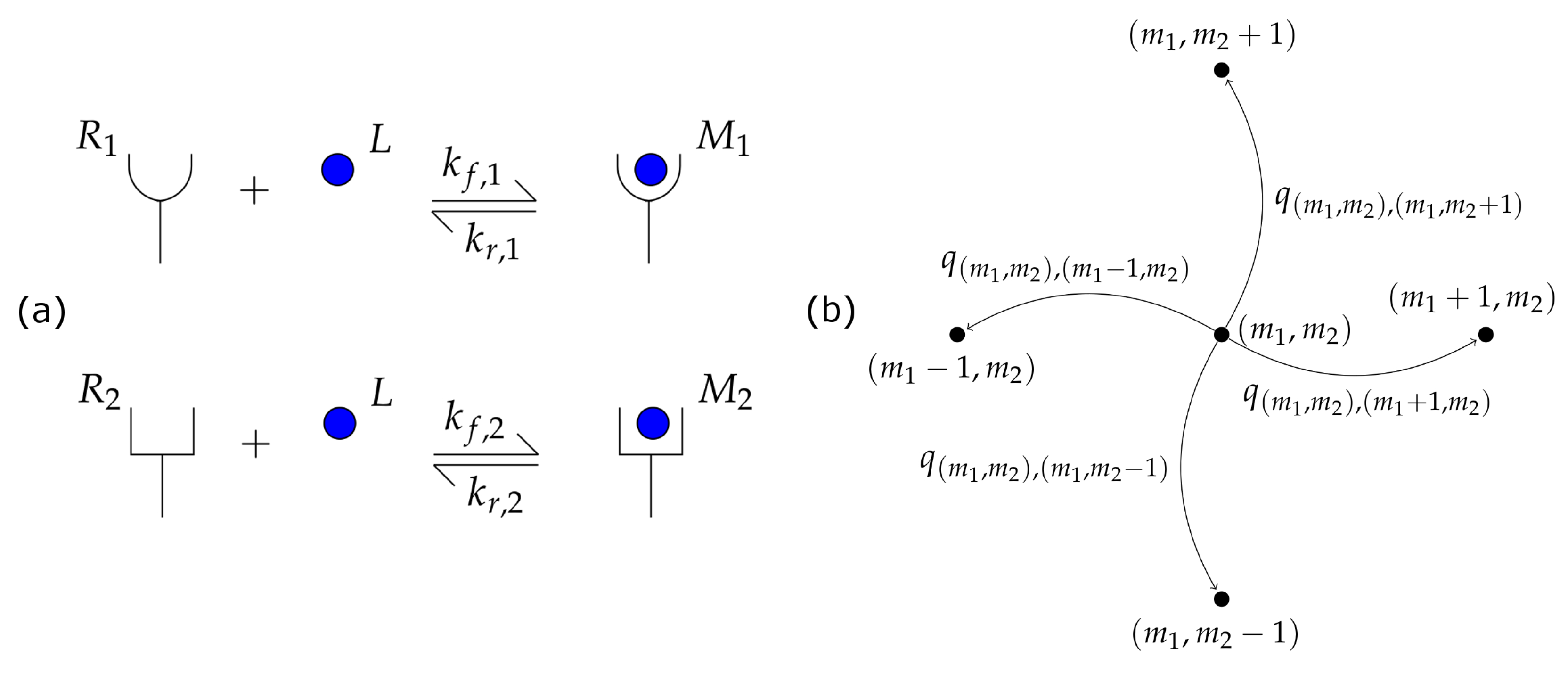
Figure 1. (a) Model reactions with two receptor types and one shared ligand. (b) Transition diagram for adjacent states in the continuous-time Markov chain (CTMC) X .
Mathematics 08 01014 g001
Figure 2. A diagram of the two-dimensional Markov process X . Each state in the process represents a number of monomers of each type ( m 1 , m 2 ) , and the transitions between states represent formation and dissociation of type 1 and type 2 monomers over time. The maximal values of m 1 and m 2 will depend on the parameters n R , 1 , n R , 2 and n L , and will determine the overall shape of S X .
Mathematics 08 01014 g002
Figure 3. Gillespie simulations of the competition process showing the effect of varying rate constants and number of molecules on the time evolution of the monomers, M 1 ( t ) and M 2 ( t ) . In the first row, for equal K d values we vary the number, n R , 2 , of type 2 receptors. In the second row, for equal number of receptors we vary K d , 2 .
Mathematics 08 01014 g003
Figure 4. Diagram for the birth-and-death process X j , j { 1 , 2 } .
Mathematics 08 01014 g004
Figure 5. Examples of how Algorithm 1 converges when n L n R , 1 + n R , 2 (left plot, n L = 50 ) and when n L < n R , 1 + n R , 2 (right plot, n L = 40 ). Iterative mean values E N C A , ( i ) [ M 1 ] , E N C A , ( i ) [ M 2 ] and N L ( i ) converge to the exact values E E M A [ M 1 ] , E E M A [ M 2 ] and E E M A [ L ] . In both plots, ϵ = 10 5 , n R , 1 = 20 , n R , 2 = 30 , K d , 1 = 1 , K d , 2 = 1 , and α = 0.2 for the right plot.
Mathematics 08 01014 g005
Figure 6. Comparison of the steady-state distributions for the EMA, NCA and MCA. The number of receptors are n R , 1 = n R , 2 = 10 2 , and K d , 1 = K d , 2 = 10 3 . The fourth and fifth columns of plots represent the absolute differences between probabilities, | π ( m 1 , m 2 ) E M A π ( m 1 , m 2 ) N C A | and | π ( m 1 , m 2 ) E M A π ( m 1 , m 2 ) M C A | , respectively.
Mathematics 08 01014 g006
Figure 7. Hellinger distance between the steady-state distributions { π ( m 1 , m 2 ) E M A } ( m 1 , m 2 ) S X and { π ( m 1 , m 2 ) M C A } ( m 1 , m 2 ) S X plotted for sampled values n R , j U ( 20 , 200 ) and K d , j = 10 x with x U ( 1 , 4 ) , for j { 1 , 2 } , and for different numbers of ligand n L { 100 , 250 , 500 } . We set the threshold parameter ϵ = 10 5 for the Moderate-Competition Approximation (MCA).
Mathematics 08 01014 g007
Figure 8. Comparison between the expected times to reach N monomers of type 2, computed using the Exact Matrix-Analytic Approach (EMA), No-Competition Approximation (NCA) and the MCA, for K d , 2 = 10 3 and different values of n L { 100 , 500 , 2500 } and K d , 1 { 10 2 , 10 3 , 10 4 } (i.e., K d , 1 K d , 2 , K d , 1 = K d , 2 or K d , 1 K d , 2 ). For all plots the number of receptors are n R , 1 = n R , 2 = 10 2 , and initial state ( m 1 , m 2 ) = ( 0 , 0 ) . P represents a percentage of the mean steady-state value, so that N = P 100 E E M A [ M 2 ] .
Mathematics 08 01014 g008
Figure 9. Relative difference between the EMA and NCA mean times to reach N monomers of type 2, plotted for 10 3 sampled parameter values in Figure 7, and for n L { 100 , 250 , 500 } .
Mathematics 08 01014 g009
Figure 10. Relative difference between the EMA and MCA mean times to reach N monomers of type 2, plotted for 10 3 sampled parameter values in Figure 7, and for n L { 100 , 250 , 500 } .
Mathematics 08 01014 g010
Figure 11. Relative difference 1 T j ( N , τ ) T S I M ( N , τ ) , j { N C A , M C A } , between the mean time T ( N , τ ) computed through the NCA and MCA approaches, and the time computed through stochastic simulations, for n L { 10 2 , 10 3 } . In these scenarios, 10 3 parameter sets have been sampled by varying the number of receptors n R 1 and n R 2 between 100 and 400, K d , 1 and K d , 2 rates vary between 10 1 and 10 4 , and setting k r , 1 = k r , 2 = 10 3 s 1 . In these examples, N = 10 and τ = k r , 1 1 , so that a monomer is considered to be productive if it lasts for longer than its average lifetime.
Mathematics 08 01014 g011
Figure 12. Absolute difference i = 1 4 | E M C A [ M i ] E S I M [ M i ] | between the mean number of monomers in steady-state computed through simulations and the MCA approach, for n L { 10 2 , 10 3 } . 10 3 parameter sets are sampled by considering the number of receptors n R , j U ( 20 , 200 ) and K d , j = 10 x with x U ( 1 , 4 ) , j { 1 , 2 , 3 , 4 } . We set k r , j = 10 3 s 1 for j { 1 , 2 , 3 , 4 } .
Mathematics 08 01014 g012
Table 1. Ranges for the parameter values and numbers of molecules in the model.
ParameterRangeUnit
K d , 1 , K d , 2 [ 1 × 10 1 1 × 10 4 ] molecules
n R , 1 , n R , 2 [ 2 × 10 1 2 × 10 2 ] molecules