Representations of Generalized Self-Shrunken Sequences

Abstract

Output sequences of the cryptographic pseudo-random number generator, known as the generalized self-shrinking generator, are obtained self-decimating Pseudo-Noise (PN)-sequences with shifted versions of themselves. In this paper, we present three different representations of this family of sequences. Two of them, the p and G-representations, are based on the parameters p and G corresponding to shifts and binary vectors, respectively, used to compute the shifted versions of the original PN-sequence. In addition, such sequences can be also computed as the binary sum of diagonals of the Sierpinski’s triangle. This is called the B-representation. Characteristics and generalities of the three representations are analyzed in detail. Under such representations, we determine some properties of these cryptographic sequences. Furthermore, these sequences form a family that has a group structure with the bit-wise XOR operation.

1. Introduction

Most of the devices that form part of the Internet-of-Things (IoT) require cryptographic security features to prevent users from data losses and the risks related to an improper use of passwords. Putting into effect cryptographic security is complicated. Most of the security systems are based on true random numbers, but their generation is really a difficult task [1,2]. Many popular random “noise” algorithms, for example, algorithms that are part of IoT devices, end up to be imperfect, showing glitches that make them predictable and vulnerable. Some weaknesses are never (publicly) found out, creating a false sense of security. The devices in which flaws are detected are those with the most flagrant errors and those most popular, for example, algorithms A5 in GSM communications cryptanalyzed in [3,4], the generator RC4 for encrypting Internet traffic cryptanalyzed in [5] or the J3Gen generator for low-cost passive RFID tags cryptanalyzed in [6]. To sum up, it is hard to build a true random number generator that can provide a strong cryptographic foundation for system security, especially for IoT devices (see [7,8]).

Pseudo-Random Number Generators (PRNGs) are reproducible and deterministic algorithms [9,10] used to generate random number sequences for cryptographic applications, such as key and nonces generation, digital signatures, and IoT security. These applications require various statistical properties, such as low autocorrelation, large period and linear complexity, rich dimensional distribution of the output sequence, and uniformity of distribution for large quantities of generated numbers (see ([11], Chapter 2) for more details).

Binary sequences produced by maximal-length Linear Feedback Shift Registers (LFSRs), called Pseudo-Noise (PN)-sequences [12], have been widely used in many diverse applications such as digital broadcasting, mobile wireless communications, e-commerce or cryptography (stream ciphers) [13,14]. In order to ensure practical cryptographic stability, it is necessary to destroy the linearity inherent to PN-sequences via different non-linear procedures.

LFSRs play an important role in the design of cryptographic PRNGs [15,16]. Among the most popular families of cryptographic sequence generators based on PN-sequences we can enumerate: non-linear filters with only one LFSR, combination generators that involve several LFSRs, clock-controlled registers where one LFSR controls the clock of the others or irregular decimation-based generators [11]. We focus our attention on this latter family.

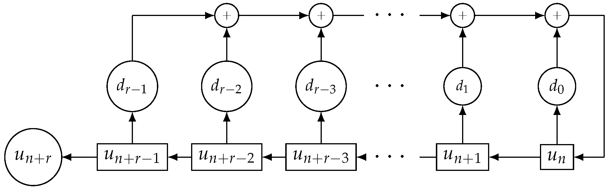
Generally speaking, the regular decimation [17] of a sequence ${\left\{a_i\right\}}_{i\ge 0}$ by distance d is a new sequence obtained by taking every d-th term of ${\left\{a_i\right\}}_{i\ge 0}$, that is, ${\left\{a_{d·i}\right\}}_{i\ge 0}$. Nevertheless, it is the irregular decimation of PN-sequences [18], which can be considered as a powerful PRNG, producing sequences with good cryptographic properties, such as long periods, good distribution of zeros and ones along the sequence, large linear complexity, and two-valued autocorrelation properties.

In the literature, there are three well-known irregularly decimated generators: the shrinking generator [19], made up of two LFSRs with different lengths, the self-shrinking generator [20], based on the self-decimation of one single PN-sequence, and the generalized self-shrinking generator (GSSG) [21], which produces a family of sequences that includes the sequence produced by the self-shrinking generator [22]. Moreover, the modified self-shrinking generator [23] and the t-modified self-shrinking generator [24] are also members of such a family. These generators are fast, easy to implement and they generate good cryptographic sequences. Therefore, they seem adequate for lightweight cryptography and, in general, low-cost applications. In [25], the authors studied the randomness of the family of sequences generated by the GSSG by means of several complete and powerful batteries of statistical tests and graphical tools. In fact, they provided a useful vision of the behavior of such sequences and proved their suitability for cryptographic applications. In [24], the relationship among the generalized self-shrinking generator and the t-modified self-shrinking generator is deeply analyzed. Furthermore, in [26], the authors studied the relationship between that generator and the modified self-shrinking generator. In [27], other authors presented an extension of the self-shrinking generator to the Galois field of $p^n$ elements with p a prime integer, that is, the p-ary Generalized Self-Shrinking Generator (p-GSSG). Furthermore, they proved that the sequences generated by this new generator have large periods and good statistical properties.

At any rate, there exist other ways to built irregularly decimated generators, for example, irregularly decimated generators based on Feedback with Carry Shift Registers (FCSRs) instead of the traditional LFSRs [28,29]. These variants of the previous generators unify in a unique structure the non-linearity inherent to the FCSRs with the irregular decimation technique. An FCSR is the arithmetic or with carry analog of an LFSR. The main difference is the fact that the elementary additions are not modulo 2 additions but with the propagation of carries. FCSRs have been used in the design of stream ciphers [30], generating pseudo-random numbers [31], and can be efficiently implemented in parallel architectures [32].

In modern algebra, group theory is the study of groups, which are sets of elements with an operation that satisfies certain axioms. The basic structure of groups can be found in many mathematical phenomena such as symmetry and certain types of transformations. Group theory has applications in robotics, computer vision/graphics and medical image analysis, physics, chemistry, computer science, and even puzzles like Rubik’s cube can be represented using group theory [33,34,35,36,37]. As we show in this paper, group theory also has applications in cryptography, since the set of output sequences of the generalized self-shrinking generator has the structure of an additive group and some of the properties of this family of sequences can be deduced as a consequence of this fact.

In this work, we study in detail three different representations of the sequences produced by the GSSG: the G-representation (introduced in [21]), the new p-representation and the B-representation (introduced in [38]). As far as we know, there are no other known representations for this kind of generators in the literature. In addition, we introduce a new way to compute the B-representation. Such a representation relates the output sequences of our generator with shifted versions of the diagonals of the binary Sierpinski’s triangle, named binomial sequences. In terms of this representation, the structural properties of some binary sequences are easily analyzed. In brief, we give a binomial expression of these sequences, providing a relation among binomial coefficients, binary sequences and group theory.

2. Fundamentals and Basic Notation

In this section, we introduce some of the main concepts related to our work: the generalized self-shrinking generator and the binomial sequences.

2.1. PN-Sequences and GSSG

Traditionally, LFSRs implement linear recurring sequences [12]. LFSRs are electronic devices in which the information units are elements of binary field ${\mathbb{F}}_2$. They are made up of r interconnected memory cells (stages) that shift their contents to their next stages and a linear feedback to the empty stage. The register is shown in Figure 1.

Generates the linear recurring sequence ${\left\{u_n\right\}}_{n\ge 0}$ (or denoted by $\left\{u_n\right\}$) given by

$$u_{n+r}=d_{r-1}{u}_{n+r-1}+d_{r-2}{u}_{n+r-2}+d_{r-3}{u}_{n+r-3}+\cdots +d_1{u}_{n+1}+d_0{u}_n,n\ge 0.$$

If the monic polynomial

$$p\left(x\right)=x^r+d_{r-1}{x}^{r-1}+d_{r-2}{x}^{r-2}+d_{r-3}{x}^{r-3}+\cdots +d_{1}x+d_0\in {\mathbb{F}}_2\left[x\right]$$

is a primitive polynomial, then the LFSR is called a maximal-length LFSR [12] and generates a PN-sequence (Pseudo Noise sequence) with maximum period $T=2^r-1$ with $2^{r-1}$ ones and $2^{r-1}-1$ zeros. This polynomial is known as the characteristic polynomial of the recurring sequence.

A common metric of the security of a sequence for its possible cryptographic application is the linear complexity [39,40,41], denoted by $LC$. Roughly speaking, the parameter $LC$ determines the portion of sequence we need in order to recover the whole sequence. In fact, $LC$ is the length of the shortest LFSR that generates such a sequence ([42], Chapter 5). Making use of the concept of recurrence, we can say that the $LC$ of a sequence is the lowest order of its linear recurrence relationship. In cryptography, linear complexity clearly must take a large value, for example, half of the period: $LC\simeq T/2$. Nowadays, values of T in the range $T\ge 2^{128}$ seem to be enough for cryptographic purposes (see specifications of the candidates in the call of NIST for lightweight cryptography primitives [43]).

Consider a PN-sequence ${\left\{u_i\right\}}_{i\ge 0}$ obtained from a maximal-length LFSR with L stages, an L-dimensional binary vector $\mathcal{G}=[g_0,g_1,g_2,...,g_{L-1}]\in {\mathbb{F}}_2^L$ and let ${\left\{v_i\right\}}_{i\ge 0}$ be the sequence defined as:

$$v_i=g_0{u}_i+g_1{u}_{i-1}+g_2{u}_{i-2}+\cdots +g_{L-1}{u}_{i-L+1}\mathrm{for}i\ge 0.$$

(1)

Next, we define a decimation rule to generate a new sequence ${\left\{s_j\right\}}_{j\ge 0}$ as follows:

$$\left\{\begin{array}{cc}\mathrm{If}{u}_i=1,\hfill & \mathrm{then}{s}_j=v_i,\hfill \\ \mathrm{If}{u}_i=0,\hfill & \mathrm{then}{v}_i\mathrm{is}\mathrm{discarded}.\hfill \end{array}\right.$$

(2)

The sequence ${\left\{s_j\right\}}_{i\ge 0}$, denoted by $S\left(\mathcal{G}\right)$, is called the generalized self-shrunken sequence, GSS-sequence or simply generalized sequence associated with $\mathcal{G}$, see [21]; and the sequence generator is called the generalized self-shrinking generator (GSSG).

Notice that when $\mathcal{G}$ runs over ${\mathbb{F}}_2^L\setminus \left\{0\right\}$ we obtain all the shifted versions of ${\left\{u_i\right\}}_{i\ge 0}$ (see Theorem 2). The set of sequences $\mathcal{S}=\left\{S\left(\mathcal{G}\right)|\mathcal{G}\in {\mathbb{F}}_2^L\right\}$ is called the family of generalized sequences based on the PN-sequence ${\left\{u_i\right\}}_{i\ge 0}$. This family $\mathcal{S}$ with the addition modulo 2, that is, with the bit-wise XOR operation, is an additive group [21]. In particular, the neutral element is the sequence $S\left(\right[0,0,\dots ,0\left]\right)=\{00000\dots \}$ and the opposite of any sequence $S\left(\mathcal{G}\right)$ is the sequence itself. Moreover, the period of every generalized sequence is a divisor of $2^{L-1}$ (the number of ones in the PN-sequence) and every sequence of this family is balanced except for the sequence identically of 1 and the null sequence ([21], Theorem 1).

Example 1.

Consider the primitive polynomial $p\left(x\right)=x^3+x^2+1$ and the PN-sequence ${\left\{u_i\right\}}_{i\ge 0}=\left\{1110100\right\}$ generated by $p\left(x\right)$ with initial state $\left\{111\right\}$. As illustration of the decimation rule given in (2) consider, for instance, $\mathcal{G}=[0,0,1]$ and the corresponding sequence ${\left\{v_i\right\}}_{i\ge 0}=\left\{0011101\right\}$. We apply the decimation rule as follows:The corresponding generalized sequence is $S\left(\right[0,0,1\left]\right)=\left\{0011\right\}$.

In

Table 1. Generalized sequences for $p\left(x\right)=x^3+x^2+1$.

$\mathcal{G}$	$\left\{{\mathit{v}}_{\mathit{i}}\right\}\mathbf{Sequence}$	Generalized Sequences
0 0 0	$0000000$	0000
0 0 1	$0011101$	0011
0 1 0	$0111010$	0110
0 1 1	$0100111$	0101
1 0 0	$1110100$	1111
1 0 1	$1101001$	1100
1 1 0	$1001110$	1001
1 1 1	$1010011$	1010
	$1110100$

, we can see the family of all generalized sequences generated by the PN-sequence ${\left\{u_i\right\}}_{i\ge 0}$. Notice that the ${\left\{v_i\right\}}_{i\ge 0}$ sequences are shifted versions of the PN-sequence $\left\{u_i\right\}$ (which appears at the bottom of the table), a fact that we will prove later in Theorem 2. The bits in bold of each sequence ${\left\{v_i\right\}}_{i\ge 0}$ are the bits of the corresponding generalized sequence.

Notice that, since the number of ones in a PN-sequence of period $2^L-1$ is $2^{L-1}$ (see [12]), the period of the generalized sequences is a divisor of $2^{L-1}$. We will see that there are always two sequences of period 1 (the identically 1 and 0 sequences), two sequences of period 2, $\left\{01010101\right\}$ and $\left\{101010101\right\}$, and the remaining sequences have the maximum period $2^{L-1}$ (although there is no mathematical proof for this last statement).

Relating to the linear complexity, in [39] Blackburn introduced an upper bound for the linear complexity of the self-shrinking generator. A generalization of this bound was introduced in [40] for the linear complexity of generalized sequences, that is, $LC\le 2^{L-1}-(L-2)$. Furthermore, we know that for all generalized sequences, except for those with period 1 and 2, we have $2^{L-2}\le LC$ (although there is no proof for this statement either).

2.2. Binomial Sequences

The binomial number $\left(\genfrac{}{}{0pt}{}{n}{i}\right)$ represents the coefficient corresponding to $x^i$ in the expansion of the polynomial ${(1+x)}^n$. For every integer $n\ge 0$, we know that $\left(\genfrac{}{}{0pt}{}{n}{0}\right)=1$ while $\left(\genfrac{}{}{0pt}{}{n}{i}\right)=0$ for $i>n$. Now, binomial sequences are introduced as follows.

Definition 1.

Given a fixed integer $k\ge 0$, the sequence ${\left\{b_n^{\left(k\right)}\right\}}_{n\ge 0}$ given by

$$b_n^{\left(k\right)}=\left\{\begin{array}{cc}0,\hfill & \mathit{if}n<k,\hfill \\ \left(\genfrac{}{}{0pt}{}{n}{k}\right)mod2,\hfill & \mathit{if}n\ge k,\hfill \end{array}\right.$$

is named the $\mathit{k}$-th binomial sequence.

In the sequel, the sequence ${\left\{b_n^{\left(k\right)}\right\}}_{n\ge 0}$ will be simply denoted by $\left\{\left(\genfrac{}{}{0pt}{}{n}{k}\right)\right\}$.

Table 2. The first 8 binomial coefficients, their binomial sequences $\left\{\left(\genfrac{}{}{0pt}{}{n}{k}\right)\right\}$, periods and complexities.

Binomial Coeff.	Binomial Sequences $$\left\{\left(\genfrac{}{}{0pt}{}{\mathit{n}}{\mathit{k}}\right)\right\}$$	Period	LC
$\left(\genfrac{}{}{0pt}{}{n}{0}\right)$	1 1 1 1 1 1 1 1 …	1	1
$\left(\genfrac{}{}{0pt}{}{n}{1}\right)$	0 1 0 1 0 1 0 1 …	2	2
$\left(\genfrac{}{}{0pt}{}{n}{2}\right)$	0 0 1 1 0 0 1 1 …	4	3
$\left(\genfrac{}{}{0pt}{}{n}{3}\right)$	0 0 0 1 0 0 0 1 …	4	4
$\left(\genfrac{}{}{0pt}{}{n}{4}\right)$	0 0 0 0 1 1 1 1 …	8	5
$\left(\genfrac{}{}{0pt}{}{n}{5}\right)$	0 0 0 0 0 1 0 1 …	8	6
$\left(\genfrac{}{}{0pt}{}{n}{6}\right)$	0 0 0 0 0 0 1 1 …	8	7
$\left(\genfrac{}{}{0pt}{}{n}{7}\right)$	0 0 0 0 0 0 0 1 …	8	8

shows the first eight binomial coefficients as well as the first eight binomial sequences with their corresponding periods and linear complexities. To check the form of the first 32 binomial sequences, see reference [38]. Moreover, recall that binomial sequences are just shifted versions of the successive diagonals of the Sierpinski’s triangle depicted in Figure 2.

Theorem 1

([38], Proposition 3, Theorem 13). The binomial sequence $\left\{\left(\genfrac{}{}{0pt}{}{n}{2^r+l}\right)\right\}$ with $0\le l<2^r$ and r being a positive integer has period of value $T=2^{r+1}$ and linear complexity of value $LC=2^r+l+1.$

Check [38] for more properties of binomial sequences.

3. Representation of Generalized Sequences

In this section, we present three different representations of the generalized self-shrunken sequences. From these representations we can obtain important information about the sequences. For instance, the binomial representation or B-representation of the generalized sequences allows us to examine the cryptographic parameters of these sequences and obtain their linear complexity; the p-representation and G-representation provide information about the shifted PN-sequences used in the decimation and allow us to define a partition of the family of generalized sequences.

It is worth saying that there exist certain advantages and disadvantages among these representations. On the one hand, the B-representation is more general and can be used for any binary sequence with a period of a power of two. On the other hand, the p-representation and the G-representation are specific representations for generalized sequences and, therefore, do not exist for other generators. However, both representations are related, being possible to get one from the other. In this section, we present some relations between the different representations.

3.1. The G-Representation of a Generalized Self-Shrunken Sequence

It is well known [12] that a PN-sequence ${\left\{u_i\right\}}_{i\ge 0}$ generated by an LFSR with primitive polynomial $p\left(x\right)$ of degree L can be represented by the trace map as follows

$$u_i=\mathrm{Tr}\left(A{\alpha }^i\right)=A{\alpha }^i+A^2{\alpha }^{2i}+A^4{\alpha }^{4i}+\cdots +A^{2^{L-1}}{\alpha }^{2^{L-1}i},i\ge 0,$$

(3)

where $A\in {\mathbb{F}}_{2^L}$ with $A\ne 0$ and $\alpha$ is a root of $p\left(x\right)$, that is, a primitive element of ${\mathbb{F}}_{2^L}$.

From now on, we consider ${\left\{u_i\right\}}_{i\ge 0}$ a PN-sequence obtained from a maximal-length LFSR with characteristic polynomial $p\left(x\right)$ of degree L.

Next theorem proves that the sequence ${\left\{v_i\right\}}_{i\ge 0}$ given in (1) is a shifted version of the PN-sequence ${\left\{u_i\right\}}_{i\ge 0}$.

Theorem 2.

Assume that ${\left\{u_i\right\}}_{i\ge 0}$ is a PN-sequence obtained from a maximal-length LFSR with characteristic polynomial $p\left(x\right)$ of degree L. If $\mathcal{G}=[g_0,g_1,\dots ,g_{L-1}]\in {\mathbb{F}}_2^L$ is a nonzero vector, then the sequence ${\left\{v_i\right\}}_{i\ge 0}$ obtained from Expression (1) is a shifted version of ${\left\{u_i\right\}}_{i\ge 0}$. In fact, ${\left\{v_i\right\}}_{i\ge 0}={\left\{u_{i-L+1+\tau \left(\mathcal{G}\right)}\right\}}_{i\ge 0},$ where $\tau \left(\mathcal{G}\right)\in \left\{0,1,\dots ,2^L-2\right\}$ such that

$${\alpha }^{\tau \left(\mathcal{G}\right)}=g_0{\alpha }^{L-1}+g_1{\alpha }^{L-2}+\cdots +g_{L-2}\alpha +g_{L-1}\in {\mathbb{F}}_{2^L}$$

with $\alpha \in {\mathbb{F}}_{2^L}$ being a root of $p\left(x\right)$.

Proof. 

From Expressions (1) and (3), it follows that

$$\begin{array}{ll}{v}_i& =g_0\left(A{\alpha }^i+A^2{\alpha }^{2i}+A^4{\alpha }^{4i}+\cdots +A^{2^{L-1}}{\alpha }^{2^{L-1}i}\right)\\ & \phantom{aa}+g_1\left(A{\alpha }^{i-1}+A^2{\alpha }^{2(i-1)}+A^4{\alpha }^{4(i-1)}+\cdots +A^{2^{L-1}}{\alpha }^{2^{L-1}(i-1)}\right)\\ & \phantom{aa}+\cdots \\ & \phantom{aa}+g_{L-2}\left(A{\alpha }^{i-L+2}+A^2{\alpha }^{2(i-L+2)}+A^4{\alpha }^{4(i-L+2)}+\cdots +A^{2^{L-1}}{\alpha }^{2^{L-1}(i-L+2)}\right)\\ & \phantom{aa}+g_{L-1}\left(A{\alpha }^{i-L+1}+A^2{\alpha }^{2(i-L+1)}+A^4{\alpha }^{4(i-L+1)}+\cdots +A^{2^{L-1}}{\alpha }^{2^{L-1}(i-L+1)}\right)\\ & =A\left({\alpha }^{i-L+1}\left(g_0{\alpha }^{L-1}+g_1{\alpha }^{i-2}+\cdots +g_{L-2}\alpha +g_{L-1}\right)\right)\\ & \phantom{aa}+A^2{\left({\alpha }^{i-L+1}\left(g_0{\alpha }^{L-1}+g_1{\alpha }^{i-2}+\cdots +g_{L-2}\alpha +g_{L-1}\right)\right)}^2\\ & \phantom{aa}+A^4{\left({\alpha }^{i-L+1}\left(g_0{\alpha }^{L-1}+g_1{\alpha }^{i-2}+\cdots +g_{L-2}\alpha +g_{L-1}\right)\right)}^4\\ & \phantom{aa}+\cdots \\ & \phantom{aa}+A^{2^{L-1}}{\left({\alpha }^{i-L+1}\left(g_0{\alpha }^{L-1}+g_1{\alpha }^{i-2}+\cdots +g_{L-2}\alpha +g_{L-1}\right)\right)}^{2^{L-1}}\\ & =A\left({\alpha }^{i-L+1}{\alpha }^{\tau \left(\mathcal{G}\right)}\right)+A^2{\left({\alpha }^{i-L+1}{\alpha }^{\tau \left(\mathcal{G}\right)}\right)}^2+A^4{\left({\alpha }^{i-L+1}{\alpha }^{\tau \left(\mathcal{G}\right)}\right)}^4+\cdots +A^{2^{L-1}}{\left({\alpha }^{i-L+1}{\alpha }^{\tau \left(\mathcal{G}\right)}\right)}^{2^{L-1}}\\ & =A\left({\alpha }^{i-L+1+\tau \left(\mathcal{G}\right)}\right)+A^2{\left({\alpha }^{i-L+1+\tau \left(\mathcal{G}\right)}\right)}^2+A^4{\left({\alpha }^{i-L+1+\tau \left(\mathcal{G}\right)}\right)}^4+\cdots +A^{2^{L-1}}{\left({\alpha }^{i-L+1+\tau \left(\mathcal{G}\right)}\right)}^{2^{L-1}}\\ & =u_{i-L+1+\tau \left(\mathcal{G}\right)}.\end{array}$$

□

Note that if in Expression (1) we consider $\mathcal{G}=[0,0,0,\dots ,0]$, then ${\left\{v_i\right\}}_{i\ge 0}$ is the null sequence.

From now on, we denote by G the decimal representation of the vector $\mathcal{G}=[g_0,g_1,g_2,...,g_{L-2},$$g_{L-1}]\in {\mathbb{F}}_2^L$, i.e.

$$G=g_0·2^{L-1}+g_1·2^{L-2}+\cdots +g_{L-2}·2+g_{L-1}.$$

Moreover, we will use indistinctly G and $\mathcal{G}$. For example $S\left(G\right)=S\left(\mathcal{G}\right)$ and $\tau \left(G\right)=\tau \left(\mathcal{G}\right)$.

Remark 1.

Since $G=3$ is the decimal representation of the binary number $[0,0,0,\dots ,0,1,1]$, we have that

$${\alpha }^{\tau \left(3\right)}=\alpha +1,$$

that is, $\tau \left(3\right)={\mathcal{Z}}_{\alpha }\left(1\right)$, where ${\mathcal{Z}}_{\alpha }\left(1\right)$ denotes the Zech logarithm of 1 with basis α.

Recall that the Zech logarithm of t with a basis of the primitive element $\alpha$ is such that ${\alpha }^{{\mathcal{Z}}_{\alpha }\left(t\right)}={\alpha }^t+1.$ Check [44] for more properties of this discrete logarithm.

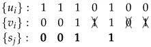
Example 2.

Consider the LFSR in which the characteristic polynomial is $p\left(x\right)=x^5+x^2+1$. For the initial state $\left\{11111\right\}$, we obtain the PN-sequence

$$\left\{1111100011011101010000100101100\right\}$$

which generates the family of generalized sequences shown in

Table 3. Generalized sequences for $p\left(x\right)=x^5+x^2+1$.

G	$\mathcal{G}$	$\left\{{\mathit{v}}_{\mathit{i}}\right\}$ Sequence	Generalized Sequence
0	00000	$\mathbf{00000}000\mathbf{00}0\mathbf{000}0000000000000\mathbf{00}00$	0000000000000000
1	00001	$\mathbf{11001}111\mathbf{10}0\mathbf{011}0111010100001\mathbf{00}10$	1100110011110000
2	00010	$\mathbf{10011}111\mathbf{00}0\mathbf{110}1110101000010\mathbf{01}01$	1001100110100101
3	00011	$\mathbf{01010}000\mathbf{10}0\mathbf{101}1001111100011\mathbf{01}11$	0101010101010101
4	00100	$\mathbf{00111}110\mathbf{00}1\mathbf{101}1101010000100\mathbf{10}11$	0011100101110010
5	00101	$\mathbf{11110}001\mathbf{10}1\mathbf{110}1010000100101\mathbf{10}01$	1111010110000010
6	00110	$\mathbf{10100}001\mathbf{00}1\mathbf{011}0011111000110\mathbf{11}10$	1010000011010111
7	00111	$\mathbf{01101}110\mathbf{10}1\mathbf{000}0100101100111\mathbf{11}00$	0110110000100111
8	01000	$\mathbf{01111}100\mathbf{01}1\mathbf{011}1010100001001\mathbf{01}10$	0111101011000001
9	01001	$\mathbf{10110}011\mathbf{11}1\mathbf{000}1101110101000\mathbf{01}00$	1011011000110001
10	01010	$\mathbf{11100}011\mathbf{01}1\mathbf{101}0100001001011\mathbf{00}11$	1110001101100100
11	01011	$\mathbf{00101}100\mathbf{11}1\mathbf{110}0011011101010\mathbf{00}01$	0010111110010100
12	01100	$\mathbf{01000}010\mathbf{01}0\mathbf{110}0111110001101\mathbf{11}01$	0100001110110011
13	01101	$\mathbf{10001}101\mathbf{11}0\mathbf{101}0000100101100\mathbf{11}11$	1000111101000011
14	01110	$\mathbf{11011}101\mathbf{01}0\mathbf{000}1001011001111\mathbf{10}00$	1101101000010110
15	01111	$\mathbf{00010}010\mathbf{11}0\mathbf{011}1110001101110\mathbf{10}10$	0001011011100110
16	10000	$\mathbf{11111}000\mathbf{11}0\mathbf{111}0101000010010\mathbf{11}00$	1111111111111111
17	10001	$\mathbf{00110}111\mathbf{01}0\mathbf{100}0010010110011\mathbf{11}10$	0011001100001111
18	10010	$\mathbf{01100}111\mathbf{11}0\mathbf{001}1011101010000\mathbf{10}01$	0110011001011010
19	10011	$\mathbf{10101}000\mathbf{01}0\mathbf{010}1100111110001\mathbf{10}11$	1010101010101010
20	10100	$\mathbf{11000}110\mathbf{11}1\mathbf{010}1000010010110\mathbf{01}11$	1100011010001101
21	10101	$\mathbf{00001}001\mathbf{01}1\mathbf{001}1111000110111\mathbf{01}01$	0000101001111101
22	10110	$\mathbf{01011}001\mathbf{11}1\mathbf{100}0110111010100\mathbf{00}10$	0101111100101000
23	10111	$\mathbf{10010}110\mathbf{01}1\mathbf{111}0001101110101\mathbf{00}00$	1001001111011000
24	11000	$\mathbf{10000}100\mathbf{10}1\mathbf{100}1111100011011\mathbf{10}10$	1000010100111110
25	11001	$\mathbf{01001}011\mathbf{00}1\mathbf{111}1000110111010\mathbf{10}00$	0100100111001110
26	11010	$\mathbf{00011}011\mathbf{10}1\mathbf{010}0001001011001\mathbf{11}11$	0001110010011011
27	11011	$\mathbf{11010}100\mathbf{00}1\mathbf{001}0110011111000\mathbf{11}01$	1101000001101011
28	11100	$\mathbf{10111}010\mathbf{10}0\mathbf{001}0010110011111\mathbf{00}01$	1011110001001100
29	11101	$\mathbf{01110}101\mathbf{00}0\mathbf{010}0101100111110\mathbf{00}11$	0111000010111100
30	11110	$\mathbf{00100}101\mathbf{10}0\mathbf{111}1100011011101\mathbf{01}00$	0010010111101001
31	11111	$\mathbf{11101}010\mathbf{00}0\mathbf{100}1011001111100\mathbf{01}10$	1110100100011001
		$\mathbf{11111}000\mathbf{11}0\mathbf{111}0101000010010\mathbf{11}00$

. The bits in bold in each sequence ${\left\{v_i\right\}}_{i\ge 0}$ correspond to the positions of the ones of the PN-sequence ${\left\{u_i\right\}}_{i\ge 0}$, which appears at the bottom of the table. Furthermore, these bits are the digits of the corresponding $S\left(\mathcal{G}\right)$ sequence. Thus, in Table 3, the sequence $S\left(\mathcal{G}\right)=S\left(\right[0,0,0,0,1\left]\right)$ corresponds to $S\left(1\right)=\left\{1100110011110000\right\}$.

Next, we consider some properties of this representation (G-representation) of the generalized sequences.

Theorem 3.

If $G=2^{L-1}$ then $S\left(G\right)$ is the identically 1 sequence.

Proof. 

Since $G=2^{L-1}$ corresponds to the vector $\mathcal{G}=[1,0,0,\dots ,0]$, from Expression (1) we have that $v_i=u_i$, for $i\ge 0$, and according to the decimation rule defined in (2), the output sequence ${\left\{s_j\right\}}_{j\ge 0}$ is the identically 1 sequence. □

Theorem 4.

For $G=0,1,\dots ,2^{L-1}-1$, the sequences $S\left(G\right)$ and $S\left(G+2^{L-1}\right)$ are complementary sequences, in the sense that $S\left(G\right)+S\left(G+2^{L-1}\right)$ is the identically 1 sequence.

Proof. 

Since the L-dimensional vector representations of G and $2^{L-1}+G$ are

$$\mathcal{G}=[0,g_1,g_2,\dots ,g_{L-1}]\mathrm{and}{\mathcal{G}}^{\prime }=[1,g_1,g_2,\dots ,g_{L-1}],$$

${\left\{v_i\right\}}_{i\ge 0}$ and ${\left\{v_i^{\prime }\right\}}_{i\ge 0}$, defined by $\mathcal{G}$ and ${\mathcal{G}}^{\prime }$ respectively, satisfy $v_i=u_i+v_i^{\prime },$ for $i\ge 0$. Now, from the decimation rule defined in (2), in order to obtain the generalized sequences $S\left(G\right)$ and $S\left(G+2^{L-1}\right)$ we only consider the case when $u_i=1$. Therefore, $s_j=1+s_j^{\prime }$, which means that the sequences $S\left(G\right)$ and $S\left(G+2^{L-1}\right)$ are complementary. □

One can easily verify that the first 16 generalized sequences in Table 3 are the complementary sequences of the last 16 sequences. This means that if we generate the first $2^{L-1}$ generalized sequences using the above method, then the remaining sequences are just the complementary sequences of the previous ones. In this way, the computation of generalized sequences is half-reduced.

3.2. The B-Representation of a Generalized Self-Shrunken Sequence

Let E be the shifting operator that acts on the terms of a sequence ${\left\{u_n\right\}}_{n\ge 0}$, that is:

$$E^k{u}_n=u_{n+k},\mathrm{for}\mathrm{all}\mathrm{integer}k\ge 0.$$

Let r be a positive integer. A sequence ${\left\{s_j\right\}}_{j\ge 0}$, of which the period is $T=2^r$ is, in turn, a particular solution of equation:

$$(E^{2^r}+1)z_n={(E+1)}^{2^r}{z}_n=0,$$

(4)

where its characteristic polynomial is ${(x+1)}^{2^r}$. According to [38,45], the solutions of Equation (4) can be written as:

$$z_n=\left(\genfrac{}{}{0pt}{}{n}{0}\right)c_0+\left(\genfrac{}{}{0pt}{}{n}{1}\right)c_1+\cdots +\left(\genfrac{}{}{0pt}{}{n}{T-1}\right)c_{T-1}\mathrm{for}n\ge 0,$$

where the coefficients $c_i\in {\mathbb{F}}_2$, 1 is the unique root of the polynomial ${(x+1)}^{2^r}$ with multiplicity $2^r$ and $\left(\genfrac{}{}{0pt}{}{n}{i}\right)$ is a binomial coefficient reduced modulo 2. Thus, ${\left\{z_n\right\}}_{n\ge 0}$ is the bit-wise XOR of T binary sequences $\left\{\left(\genfrac{}{}{0pt}{}{n}{i}\right)\right\}$ weighted by T binary coefficients $c_i$. Hence, all the solutions of the difference equation written in (4) are sums of binomial sequences. In particular, every solution ${\left\{z_n\right\}}_{n\ge 0}$ can be written as:

$$\left\{z_n\right\}=\sum _{i=0}^{\nu }{c}_i\left\{\left(\genfrac{}{}{0pt}{}{n}{i}\right)\right\},$$

(5)

with $c_i\in {\mathbb{F}}_2$, $i=0,1,\dots ,\nu$, where $\nu$ is the greatest value i for which $c_{\nu }\ne 0$ while $c_i=0$ for $\nu <i<T$. Expression (5) is the binomial representation (or B-representation) of the sequence ${\left\{z_n\right\}}_{n\ge 0}$.

In terms of this representation, the parameters of the sequence ${\left\{z_n\right\}}_{n\ge 0}$ can be easily analyzed. Indeed, the period of ${\left\{z_n\right\}}_{n\ge 0}$ is the period of the binomial sequence $\left\{\left(\genfrac{}{}{0pt}{}{n}{\nu }\right)\right\}$ and the linear complexity of ${\left\{z_n\right\}}_{n\ge 0}$ is the linear complexity of the binomial sequence $\left\{\left(\genfrac{}{}{0pt}{}{n}{\nu }\right)\right\}$, that is $LC=\nu +1$ (see Theorem 1).

As a consequence we can recall the following result.

Theorem 5

([38], Theorem 2). Given the binary sequence ${\left\{z_n\right\}}_{n\ge 0}$ with period $T=2^r$, where r is a positive integer, and linear complexity $LC$, such sequence can be written as a linear combination of binomial sequences, that is, ${\sum }_{i=0}^{LC-1}{c}_i\left\{\left(\genfrac{}{}{0pt}{}{n}{i}\right)\right\}$, $c_i\in {\mathbb{F}}_2$.

We will use indistinctly the notation ${\sum }_{i=0}^{LC-1}{c}_i\left\{\left(\genfrac{}{}{0pt}{}{n}{i}\right)\right\}$ or $\left\{{\sum }_{i=0}^{LC-1}{c}_i\left(\genfrac{}{}{0pt}{}{n}{i}\right)\right\}$ to denote the B-representation of the sequence ${\left\{z_n\right\}}_{n\ge 0}$. Notice that, in the B-representation, the term with the highest index is $\left(\genfrac{}{}{0pt}{}{n}{LC-1}\right)$. This means that the last term provides the $LC$ of the sequence. We denote by $\left\{0\right\}$ the B-representation of the null sequence.

Example 3.

Consider the sequence $\left\{z_n\right\}=\{11100100\dots \}$ with period $T=8$. This sequence can be also written as a linear combination of the sequences $\left\{\left(\genfrac{}{}{0pt}{}{n}{0}\right)\right\}+\left\{\left(\genfrac{}{}{0pt}{}{n}{3}\right)\right\}+\left\{\left(\genfrac{}{}{0pt}{}{n}{4}\right)\right\}+\left\{\left(\genfrac{}{}{0pt}{}{n}{5}\right)\right\}$:

$$\begin{array}{lll}& \left\{\left(\genfrac{}{}{0pt}{}{n}{5}\right)\right\}:& \{00000101\dots \}\\ +& \left\{\left(\genfrac{}{}{0pt}{}{n}{4}\right)\right\}:& \{00001111\dots \}\\ & \left\{\left(\genfrac{}{}{0pt}{}{n}{3}\right)\right\}:& \{00010001\dots \}\\ & \left\{\left(\genfrac{}{}{0pt}{}{n}{0}\right)\right\}:& \{11111111\dots \}\\ & \left\{z_n\right\}:& \{11100100\dots \}\end{array}$$

Since the binomial sequence $\left\{\left(\genfrac{}{}{0pt}{}{n}{\nu }\right)\right\}$ (the term with highest index) is $\left\{\left(\genfrac{}{}{0pt}{}{n}{5}\right)\right\}$, then the linear complexity of $\left\{z_n\right\}$ will be $LC=6$. In the same way, its period $T=8$ coincides with the period of the sequence $\left\{\left(\genfrac{}{}{0pt}{}{n}{5}\right)\right\}$.

In [38], the authors proposed an algorithm to compute the B-representation of any sequence with a period of the power of two. Here, our aim is to propose another method to compute the B-representation of a generalized sequence. Next, we give a method to obtain this representation from any binary sequence of period a power of two. For this, we need to define a binary matrix called the binomial matrix, which is similar to the construction of a binary Hadamard matrix. Consider $H_0=\left[1\right]$ the binomial matrix for $t=0$, that is, a matrix of size $2^0\times 2^0$. We construct the binomial matrix for $t=1$ as follows

$$H_1=\left[\begin{array}{cc}{H}_0& H_0\\ 0& H_0\end{array}\right]=\left[\begin{array}{cc}1& 1\\ 0& 1\end{array}\right],$$

which has size $2^1\times 2^1$. In general, we obtain the binomial matrix for t as

$$H_t=\left[\begin{array}{cc}{H}_{t-1}& H_{t-1}\\ 0_{t-1}& H_{t-1}\end{array}\right]$$

where $H_{t-1}$ is the binomial matrix of size $2^{t-1}\times 2^{t-1}$ and $0_{t-1}$ is the null matrix of the same size.

Let ${\left\{s_n\right\}}_{n\ge 0}$ be a binary sequence of period $T=2^t$. Given the binomial matrix $H_t$ of size $2^t\times 2^t$, we construct the binary vector

$$B=[s_0,s_1,\dots ,s_{2^t-1}]·H_{t}mod2.$$

(6)

The support of the vector B, denoted by $\mathrm{supp}\left(B\right)$, is the set of indices of the nonzero entries of B, considering the first position as the 0 position. Then, we define the B-representation of ${\left\{s_n\right\}}_{n\ge 0}$, denoted by $B\left(\left\{s_n\right\}\right)$, as the sequence given by the addition of the binomial sequences $\left\{\left(\genfrac{}{}{0pt}{}{n}{i}\right)\right\}$, for $i\in \mathrm{supp}\left(B\right)$, that is

$$\begin{array}{c}\hfill B\left([s_0,s_1,\dots ,s_{2^t-1}]\right)=\sum _{i\in \mathrm{supp}\left(B\right)}\left\{\left(\genfrac{}{}{0pt}{}{n}{i}\right)\right\}.\end{array}$$

(7)

Notice that, as a consequence of Expression (6), we can only compute the B-representation of binary sequences of period $T=2^t$. In particular, we can always obtain the B-representation of any GSS-sequence since the family of generalized sequences consists of $2^L$ sequences with periods power of two (see [21]).

The following example helps us to understand this construction.

Example 4.

Consider the binary sequence $\left\{s_n\right\}=\{11100100\dots \}$ given in Example 3 in which the B-representation is $\left\{\left(\genfrac{}{}{0pt}{}{n}{0}\right)+\left(\genfrac{}{}{0pt}{}{n}{3}\right)+\left(\genfrac{}{}{0pt}{}{n}{4}\right)+\left(\genfrac{}{}{0pt}{}{n}{5}\right)\right\}$. We check it using the method defined previously. The period of the sequence is $2^3$, so we must construct the binomial matrix for $t=3$, that is

$$H_3=\left[\begin{array}{cccccccc}1& 1& 1& 1& 1& 1& 1& 1\\ 0& 1& 0& 1& 0& 1& 0& 1\\ 0& 0& 1& 1& 0& 0& 1& 1\\ 0& 0& 0& 1& 0& 0& 0& 1\\ 0& 0& 0& 0& 1& 1& 1& 1\\ 0& 0& 0& 0& 0& 1& 0& 1\\ 0& 0& 0& 0& 0& 0& 1& 1\\ 0& 0& 0& 0& 0& 0& 0& 1\end{array}\right].$$

From Expression (6), we have that

$$B=[s_0,s_1,\dots ,s_7]·H_3=\left[10011100\right]$$

and, therefore, $\mathrm{supp}\left(B\right)=\{0,3,4,5\}$. So, from Expression (7), we have that $B\left([s_0,s_1,\dots ,s_7]\right)=\left\{\left(\genfrac{}{}{0pt}{}{n}{0}\right)+\left(\genfrac{}{}{0pt}{}{n}{3}\right)+\left(\genfrac{}{}{0pt}{}{n}{4}\right)+\left(\genfrac{}{}{0pt}{}{n}{5}\right)\right\}$, as we expected.

Recall that the columns of the binomial matrix (read from right to left) correspond to the successive diagonals of the Sierpinski’s triangle in Figure 2. Thus, the binary vector B in Expression (6) is just the product of $[s_0,s_1,\dots ,s_{2^t-1}]$ by the diagonals of such a triangle.

We know that the generalized sequences have periods of the form $2^r$, with $r<L$. Therefore, we can express the generalized sequences as a finite sum of binomial sequences.

The following result is an immediate consequence of Theorems 4 and 3.

Theorem 6.

For $G=0,1,\dots ,2^{L-1}-1$, the B-representations of $S\left(G\right)$ and $S\left(G+2^{L-1}\right)$ are equal except for the term $\left\{\left(\genfrac{}{}{0pt}{}{n}{0}\right)\right\}$. Furthermore, the B-representation of $S\left(2^{L-1}\right)$ is exactly $\left\{\left(\genfrac{}{}{0pt}{}{n}{0}\right)\right\}$.

This means that if we have the B-representations of the first $2^{L-1}$ generalized sequences, then the B-representations of the remaining $2^{L-1}$ sequences are the same ones except for the term $\left(\genfrac{}{}{0pt}{}{n}{0}\right)$. In this way, the computation of generalized sequences is half-reduced.

Example 5.

Consider again the generalized sequences obtained in Example 2. In

Table 4. Binomial representation for the generalized sequences of $p\left(x\right)=x^5+x^2+1$.

G	Generalized Sequence	B-Representation
0	0000000000000000	{$0$}
1	1 1 0 0 1 1 0 0 1 1 1 1 0 0 0 0	$\left\{\left(\genfrac{}{}{0pt}{}{n}{0}\right)+\left(\genfrac{}{}{0pt}{}{n}{2}\right)+\left(\genfrac{}{}{0pt}{}{n}{10}\right)+\left(\genfrac{}{}{0pt}{}{n}{12}\right)\right\}$
2	1 0 0 1 1 0 0 1 1 0 1 0 0 1 0 1	$\left\{\left(\genfrac{}{}{0pt}{}{n}{0}\right)+\left(\genfrac{}{}{0pt}{}{n}{1}\right)+\left(\genfrac{}{}{0pt}{}{n}{2}\right)+\left(\genfrac{}{}{0pt}{}{n}{10}\right)+\left(\genfrac{}{}{0pt}{}{n}{12}\right)\right\}$
3	0 1 0 1 0 1 0 1 0 1 0 1 0 1 0 1	$\left\{\left(\genfrac{}{}{0pt}{}{n}{1}\right)\right\}$
4	0 0 1 1 1 0 0 1 0 1 1 1 0 0 1 0	$\left\{\left(\genfrac{}{}{0pt}{}{n}{2}\right)+\left(\genfrac{}{}{0pt}{}{n}{4}\right)+\left(\genfrac{}{}{0pt}{}{n}{5}\right)+\left(\genfrac{}{}{0pt}{}{n}{9}\right)+\left(\genfrac{}{}{0pt}{}{n}{11}\right)+\left(\genfrac{}{}{0pt}{}{n}{12}\right)\right\}$
5	1 1 1 1 0 1 0 1 1 0 0 0 0 0 1 0	$\left\{\left(\genfrac{}{}{0pt}{}{n}{0}\right)+\left(\genfrac{}{}{0pt}{}{n}{4}\right)+\left(\genfrac{}{}{0pt}{}{n}{5}\right)+\left(\genfrac{}{}{0pt}{}{n}{9}\right)+\left(\genfrac{}{}{0pt}{}{n}{10}\right)+\left(\genfrac{}{}{0pt}{}{n}{11}\right)\right\}$
6	1 0 1 0 0 0 0 0 1 1 0 1 0 1 1 1	$\left\{\left(\genfrac{}{}{0pt}{}{n}{0}\right)+\left(\genfrac{}{}{0pt}{}{n}{1}\right)+\left(\genfrac{}{}{0pt}{}{n}{4}\right)+\left(\genfrac{}{}{0pt}{}{n}{5}\right)+\left(\genfrac{}{}{0pt}{}{n}{9}\right)+\left(\genfrac{}{}{0pt}{}{n}{10}\right)+\left(\genfrac{}{}{0pt}{}{n}{11}\right)\right\}$
7	0 1 1 0 1 1 0 0 0 0 1 0 0 1 1 1	$\left\{\left(\genfrac{}{}{0pt}{}{n}{1}\right)+\left(\genfrac{}{}{0pt}{}{n}{2}\right)+\left(\genfrac{}{}{0pt}{}{n}{4}\right)+\left(\genfrac{}{}{0pt}{}{n}{5}\right)+\left(\genfrac{}{}{0pt}{}{n}{9}\right)+\left(\genfrac{}{}{0pt}{}{n}{11}\right)+\left(\genfrac{}{}{0pt}{}{n}{12}\right)\right\}$
8	0 1 1 1 1 0 1 0 1 1 0 0 0 0 0 1	$\left\{\left(\genfrac{}{}{0pt}{}{n}{1}\right)+\left(\genfrac{}{}{0pt}{}{n}{2}\right)+\left(\genfrac{}{}{0pt}{}{n}{3}\right)+\left(\genfrac{}{}{0pt}{}{n}{4}\right)+\left(\genfrac{}{}{0pt}{}{n}{6}\right)+\left(\genfrac{}{}{0pt}{}{n}{7}\right)+\left(\genfrac{}{}{0pt}{}{n}{8}\right)+\left(\genfrac{}{}{0pt}{}{n}{9}\right)+\left(\genfrac{}{}{0pt}{}{n}{11}\right)\right\}$
9	1 0 1 1 0 1 1 0 0 0 1 1 0 0 0 1	$\left\{\left(\genfrac{}{}{0pt}{}{n}{0}\right)+\left(\genfrac{}{}{0pt}{}{n}{1}\right)+\left(\genfrac{}{}{0pt}{}{n}{3}\right)+\left(\genfrac{}{}{0pt}{}{n}{4}\right)+\left(\genfrac{}{}{0pt}{}{n}{6}\right)+\left(\genfrac{}{}{0pt}{}{n}{7}\right)+\left(\genfrac{}{}{0pt}{}{n}{8}\right)+\left(\genfrac{}{}{0pt}{}{n}{9}\right)+\left(\genfrac{}{}{0pt}{}{n}{10}\right)+\left(\genfrac{}{}{0pt}{}{n}{11}\right)+\left(\genfrac{}{}{0pt}{}{n}{12}\right)\right\}$
10	1 1 1 0 0 0 1 1 0 1 1 0 0 1 0 0	$\left\{\left(\genfrac{}{}{0pt}{}{n}{0}\right)+\left(\genfrac{}{}{0pt}{}{n}{3}\right)+\left(\genfrac{}{}{0pt}{}{n}{4}\right)+\left(\genfrac{}{}{0pt}{}{n}{6}\right)+\left(\genfrac{}{}{0pt}{}{n}{7}\right)+\left(\genfrac{}{}{0pt}{}{n}{8}\right)+\left(\genfrac{}{}{0pt}{}{n}{9}\right)+\left(\genfrac{}{}{0pt}{}{n}{10}\right)+\left(\genfrac{}{}{0pt}{}{n}{11}\right)+\left(\genfrac{}{}{0pt}{}{n}{12}\right)\right\}$
11	0 0 1 0 1 1 1 1 1 0 0 1 0 1 0 0	$\left\{\left(\genfrac{}{}{0pt}{}{n}{2}\right)+\left(\genfrac{}{}{0pt}{}{n}{3}\right)+\left(\genfrac{}{}{0pt}{}{n}{4}\right)+\left(\genfrac{}{}{0pt}{}{n}{6}\right)+\left(\genfrac{}{}{0pt}{}{n}{7}\right)+\left(\genfrac{}{}{0pt}{}{n}{8}\right)+\left(\genfrac{}{}{0pt}{}{n}{9}\right)+\left(\genfrac{}{}{0pt}{}{n}{11}\right)\right\}$
12	0 1 0 0 0 0 1 1 1 0 1 1 0 0 1 1	$\left\{\left(\genfrac{}{}{0pt}{}{n}{1}\right)+\left(\genfrac{}{}{0pt}{}{n}{3}\right)+\left(\genfrac{}{}{0pt}{}{n}{5}\right)+\left(\genfrac{}{}{0pt}{}{n}{6}\right)+\left(\genfrac{}{}{0pt}{}{n}{7}\right)+\left(\genfrac{}{}{0pt}{}{n}{8}\right)+\left(\genfrac{}{}{0pt}{}{n}{12}\right)\right\}$
13	1 0 0 0 1 1 1 1 0 1 0 0 0 0 1 1	$\left\{\left(\genfrac{}{}{0pt}{}{n}{0}\right)+\left(\genfrac{}{}{0pt}{}{n}{1}\right)+\left(\genfrac{}{}{0pt}{}{n}{2}\right)+\left(\genfrac{}{}{0pt}{}{n}{3}\right)+\left(\genfrac{}{}{0pt}{}{n}{5}\right)+\left(\genfrac{}{}{0pt}{}{n}{6}\right)+\left(\genfrac{}{}{0pt}{}{n}{7}\right)+\left(\genfrac{}{}{0pt}{}{n}{8}\right)+\left(\genfrac{}{}{0pt}{}{n}{10}\right)\right\}$
14	1 1 0 1 1 0 1 0 0 0 0 1 0 1 1 0	$\left\{\left(\genfrac{}{}{0pt}{}{n}{0}\right)+\left(\genfrac{}{}{0pt}{}{n}{2}\right)+\left(\genfrac{}{}{0pt}{}{n}{3}\right)+\left(\genfrac{}{}{0pt}{}{n}{5}\right)+\left(\genfrac{}{}{0pt}{}{n}{6}\right)+\left(\genfrac{}{}{0pt}{}{n}{7}\right)+\left(\genfrac{}{}{0pt}{}{n}{8}\right)+\left(\genfrac{}{}{0pt}{}{n}{10}\right)\right\}$
15	0 0 0 1 0 1 1 0 1 1 1 0 0 1 1 0	$\left\{\left(\genfrac{}{}{0pt}{}{n}{3}\right)+\left(\genfrac{}{}{0pt}{}{n}{5}\right)+\left(\genfrac{}{}{0pt}{}{n}{6}\right)+\left(\genfrac{}{}{0pt}{}{n}{7}\right)+\left(\genfrac{}{}{0pt}{}{n}{8}\right)+\left(\genfrac{}{}{0pt}{}{n}{12}\right)\right\}$
16	1 1 1 1 1 1 1 1 1 1 1 1 1 1 1 1	$\left\{\left(\genfrac{}{}{0pt}{}{n}{0}\right)\right\}$
17	0 0 1 1 0 0 1 1 0 0 0 0 1 1 1 1	$\left\{\left(\genfrac{}{}{0pt}{}{n}{2}\right)+\left(\genfrac{}{}{0pt}{}{n}{10}\right)+\left(\genfrac{}{}{0pt}{}{n}{12}\right)\right\}$
18	0 1 1 0 0 1 1 0 0 1 0 1 1 0 1 0	$\left\{\left(\genfrac{}{}{0pt}{}{n}{1}\right)+\left(\genfrac{}{}{0pt}{}{n}{2}\right)+\left(\genfrac{}{}{0pt}{}{n}{10}\right)+\left(\genfrac{}{}{0pt}{}{n}{12}\right)\right\}$
19	1 0 1 0 1 0 1 0 1 0 1 0 1 0 1 0	$\left\{\left(\genfrac{}{}{0pt}{}{n}{0}\right)+\left(\genfrac{}{}{0pt}{}{n}{1}\right)\right\}$
20	1 1 0 0 0 1 1 0 1 0 0 0 1 1 0 1	$\left\{\left(\genfrac{}{}{0pt}{}{n}{0}\right)+\left(\genfrac{}{}{0pt}{}{n}{2}\right)+\left(\genfrac{}{}{0pt}{}{n}{4}\right)+\left(\genfrac{}{}{0pt}{}{n}{5}\right)+\left(\genfrac{}{}{0pt}{}{n}{9}\right)+\left(\genfrac{}{}{0pt}{}{n}{11}\right)+\left(\genfrac{}{}{0pt}{}{n}{12}\right)\right\}$
21	0 0 0 0 1 0 1 0 0 1 1 1 1 1 0 1	$\left\{\left(\genfrac{}{}{0pt}{}{n}{4}\right)+\left(\genfrac{}{}{0pt}{}{n}{5}\right)+\left(\genfrac{}{}{0pt}{}{n}{9}\right)+\left(\genfrac{}{}{0pt}{}{n}{10}\right)+\left(\genfrac{}{}{0pt}{}{n}{11}\right)\right\}$
22	0 1 0 1 1 1 1 1 0 0 1 0 1 0 0 0	$\left\{\left(\genfrac{}{}{0pt}{}{n}{1}\right)+\left(\genfrac{}{}{0pt}{}{n}{4}\right)+\left(\genfrac{}{}{0pt}{}{n}{5}\right)+\left(\genfrac{}{}{0pt}{}{n}{9}\right)+\left(\genfrac{}{}{0pt}{}{n}{10}\right)+\left(\genfrac{}{}{0pt}{}{n}{11}\right)\right\}$
23	1 0 0 1 0 0 1 1 1 1 0 1 1 0 0 0	$\left\{\left(\genfrac{}{}{0pt}{}{n}{0}\right)+\left(\genfrac{}{}{0pt}{}{n}{1}\right)+\left(\genfrac{}{}{0pt}{}{n}{2}\right)+\left(\genfrac{}{}{0pt}{}{n}{4}\right)+\left(\genfrac{}{}{0pt}{}{n}{5}\right)+\left(\genfrac{}{}{0pt}{}{n}{9}\right)+\left(\genfrac{}{}{0pt}{}{n}{11}\right)+\left(\genfrac{}{}{0pt}{}{n}{12}\right)\right\}$
24	1 0 0 0 0 1 0 1 0 0 1 1 1 1 1 0	$\left\{\left(\genfrac{}{}{0pt}{}{n}{0}\right)+\left(\genfrac{}{}{0pt}{}{n}{1}\right)+\left(\genfrac{}{}{0pt}{}{n}{2}\right)+\left(\genfrac{}{}{0pt}{}{n}{3}\right)+\left(\genfrac{}{}{0pt}{}{n}{4}\right)+\left(\genfrac{}{}{0pt}{}{n}{6}\right)+\left(\genfrac{}{}{0pt}{}{n}{7}\right)+\left(\genfrac{}{}{0pt}{}{n}{8}\right)+\left(\genfrac{}{}{0pt}{}{n}{9}\right)+\left(\genfrac{}{}{0pt}{}{n}{11}\right)\right\}$
25	0 1 0 0 1 0 0 1 1 1 0 0 1 1 1 0	$\left\{\left(\genfrac{}{}{0pt}{}{n}{1}\right)+\left(\genfrac{}{}{0pt}{}{n}{3}\right)+\left(\genfrac{}{}{0pt}{}{n}{4}\right)+\left(\genfrac{}{}{0pt}{}{n}{6}\right)+\left(\genfrac{}{}{0pt}{}{n}{7}\right)+\left(\genfrac{}{}{0pt}{}{n}{8}\right)+\left(\genfrac{}{}{0pt}{}{n}{9}\right)+\left(\genfrac{}{}{0pt}{}{n}{10}\right)+\left(\genfrac{}{}{0pt}{}{n}{11}\right)+\left(\genfrac{}{}{0pt}{}{n}{12}\right)\right\}$
26	0 0 0 1 1 1 0 0 1 0 0 1 1 0 1 1	$\left\{\left(\genfrac{}{}{0pt}{}{n}{3}\right)+\left(\genfrac{}{}{0pt}{}{n}{4}\right)+\left(\genfrac{}{}{0pt}{}{n}{6}\right)+\left(\genfrac{}{}{0pt}{}{n}{7}\right)+\left(\genfrac{}{}{0pt}{}{n}{8}\right)+\left(\genfrac{}{}{0pt}{}{n}{9}\right)+\left(\genfrac{}{}{0pt}{}{n}{10}\right)+\left(\genfrac{}{}{0pt}{}{n}{11}\right)+\left(\genfrac{}{}{0pt}{}{n}{12}\right)\right\}$
27	1 1 0 1 0 0 0 0 0 1 1 0 1 0 1 1	$\left\{\left(\genfrac{}{}{0pt}{}{n}{0}\right)+\left(\genfrac{}{}{0pt}{}{n}{2}\right)+\left(\genfrac{}{}{0pt}{}{n}{3}\right)+\left(\genfrac{}{}{0pt}{}{n}{4}\right)+\left(\genfrac{}{}{0pt}{}{n}{6}\right)+\left(\genfrac{}{}{0pt}{}{n}{7}\right)+\left(\genfrac{}{}{0pt}{}{n}{8}\right)+\left(\genfrac{}{}{0pt}{}{n}{9}\right)+\left(\genfrac{}{}{0pt}{}{n}{11}\right)\right\}$
28	1 0 1 1 1 1 0 0 0 1 0 0 1 1 0 0	$\left\{\left(\genfrac{}{}{0pt}{}{n}{0}\right)+\left(\genfrac{}{}{0pt}{}{n}{1}\right)+\left(\genfrac{}{}{0pt}{}{n}{3}\right)+\left(\genfrac{}{}{0pt}{}{n}{5}\right)+\left(\genfrac{}{}{0pt}{}{n}{6}\right)+\left(\genfrac{}{}{0pt}{}{n}{7}\right)+\left(\genfrac{}{}{0pt}{}{n}{8}\right)+\left(\genfrac{}{}{0pt}{}{n}{12}\right)\right\}$
29	0 1 1 1 0 0 0 0 1 0 1 1 1 1 0 0	$\left\{\left(\genfrac{}{}{0pt}{}{n}{1}\right)+\left(\genfrac{}{}{0pt}{}{n}{2}\right)+\left(\genfrac{}{}{0pt}{}{n}{3}\right)+\left(\genfrac{}{}{0pt}{}{n}{5}\right)+\left(\genfrac{}{}{0pt}{}{n}{6}\right)+\left(\genfrac{}{}{0pt}{}{n}{7}\right)+\left(\genfrac{}{}{0pt}{}{n}{8}\right)+\left(\genfrac{}{}{0pt}{}{n}{10}\right)\right\}$
30	0 0 1 0 0 1 0 1 1 1 1 0 1 0 0 1	$\left\{\left(\genfrac{}{}{0pt}{}{n}{2}\right)+\left(\genfrac{}{}{0pt}{}{n}{3}\right)+\left(\genfrac{}{}{0pt}{}{n}{5}\right)+\left(\genfrac{}{}{0pt}{}{n}{6}\right)+\left(\genfrac{}{}{0pt}{}{n}{7}\right)+\left(\genfrac{}{}{0pt}{}{n}{8}\right)+\left(\genfrac{}{}{0pt}{}{n}{10}\right)\right\}$
31	1 1 1 0 1 0 0 1 0 0 0 1 1 0 0 1	$\left\{\left(\genfrac{}{}{0pt}{}{n}{0}\right)+\left(\genfrac{}{}{0pt}{}{n}{3}\right)+\left(\genfrac{}{}{0pt}{}{n}{5}\right)+\left(\genfrac{}{}{0pt}{}{n}{6}\right)+\left(\genfrac{}{}{0pt}{}{n}{7}\right)+\left(\genfrac{}{}{0pt}{}{n}{8}\right)+\left(\genfrac{}{}{0pt}{}{n}{12}\right)\right\}$

, we can find the B-representation of each one of these generalized sequences. As we saw in Section 3.1, the last 16 generalized sequences in Table 3 are the complementary sequences of the first 16 sequences and then, from Theorem 6, the B-representation of them is the same except for the term $\left\{\left(\genfrac{}{}{0pt}{}{n}{0}\right)\right\}$. Furthermore, the B-representation of $S\left(16\right)$ is $\left\{\left(\genfrac{}{}{0pt}{}{n}{0}\right)\right\}$, as expected.

Some other properties of the family of generalized sequences can be deduced from the B-representation. We study these properties in detail in Section 4.

3.3. The p-Representation of a Generalized Self-Shrunken Sequence

In this subsection, we define a new representation of generalized sequences which gives us information of the shifted sequences employed in the decimation rule defined in (2).

From Theorem 2, we have that the sequence ${\left\{v_i\right\}}_{i\ge 0}$ is a shifted version of the PN-sequence ${\left\{u_i\right\}}_{i\ge 0}$. Therefore, instead of considering the vector $\mathcal{G}$ in Expression (1) to construct ${\left\{v_i\right\}}_{i\ge 0}$, we can simply consider the successive shifted versions of ${\left\{u_i\right\}}_{i\ge 0}$ and apply in each case the decimation rule given in (2).

Let us consider the p-shifted version of the PN-sequence ${\left\{u_i\right\}}_{i\ge 0}$ with $0\le p<2^L-1$. Applying the decimation rule given in (2), we construct the corresponding generalized sequence, which we denote by $S\left\{p\right\}$. This new representation of a generalized sequence is called p-representation.

One of the consequences of the group structure of $\mathcal{S}$ is that the sum of two generalized sequences is another generalized sequence. The following theorem allows us to obtain the p-representation of the resulting generalized sequence from the p-representations of two generalized sequences given.

Theorem 7.

Consider that ${\left\{u_i\right\}}_{i\ge 0}$ is the PN-sequence of an LFSR with primitive characteristic polynomial $p\left(x\right)$ of degree L and $\alpha \in {\mathbb{F}}_{2^L}$ is a root of $p\left(x\right)$. Then, the sum of two generalized sequences obtained with shifts $d_1$ and $d_2$ is another generalized sequence with shift $d_1+{\mathcal{Z}}_{\alpha }\left(d_2-d_1\right)$, i.e,

$$S\left\{d_1\right\}+S\left\{d_2\right\}=S\{d_1+{\mathcal{Z}}_{\alpha }\left(d_2-d_1\right)\},$$

where ${\mathcal{Z}}_{\alpha }(·)$ is as before the Zech logarithm with basis α.

Proof. 

Assume that $S\left\{d_1\right\}=\left\{s_j\right\}$ and $S\left\{d_2\right\}=\left\{{\tilde{s}}_j\right\}$ are two generalized sequences obtained from the PN-sequence $\left\{u_i\right\}$.

According to the decimation rule given in (2), if $\mathrm{supp}\left(\left\{u_i\right\}\right)=\left\{i_0,i_1,\dots ,i_{2^{L-1}-1}\right\}$, then we have that $s_j=u_{d_1+i_j}$ and ${\tilde{s}}_j=u_{d_2+i_j}$.

We have seen in Expression (3) that every element of $\left\{u_i\right\}$ can be expressed as

$$u_i=A{\alpha }^i+A^2{\alpha }^{2i}+A^4{\alpha }^{4i}+\cdots +A^{2^{L-1}}{\alpha }^{2^{L-1}i},$$

where $A\in {\mathbb{F}}_{2^L}$ with $A\ne 0$. Therefore, we have that:

$$\begin{array}{cc}\hfill u_{d_1+i_j}=& A{\alpha }^{d_1+i_j}+A^2{\alpha }^{2(d_1+i_j)}+A^4{\alpha }^{4(d_1+i_j)}+\dots +A^{2^{L-1}}{\alpha }^{2^{L-1}(d_1+i_j)}\hfill \\ \hfill u_{d_2+i_j}=& A{\alpha }^{d_2+i_j}+A^2{\alpha }^{2(d_2+i_j)}+A^4{\alpha }^{4(d_2+i_j)}+\dots +A^{2^{L-1}}{\alpha }^{2^{L-1}(d_2+i_j)}.\hfill \end{array}$$

Bit-wise XORing both sequences $\left\{s_j\right\}+\left\{{\tilde{s}}_j\right\}=\left\{u_{d_1+i_j}\right\}+\left\{u_{d_2+i_j}\right\}=\{u_{d_1+i_j}+u_{d_2+i_j}\}$ we get:

$$\begin{array}{cc}\hfill u_{d_1+i_j}+u_{d_2+i_j}& =A{\alpha }^{i_j}({\alpha }^{d_1}+{\alpha }^{d_2})+A^2{\alpha }^{2i_j}({\alpha }^{2d_1}+{\alpha }^{2d_2})+\dots +A^{2^{L-1}}{\alpha }^{2^{L-1}{i}_j}({\alpha }^{2^{L-1}{d}_1}+{\alpha }^{2^{L-1}{d}_2})\hfill \\ \hfill & =A{\alpha }^{i_j+d_1+{\mathcal{Z}}_{\alpha }\left(d_2-d_1\right)}+A^2{\alpha }^{2(i_j+d_1+{\mathcal{Z}}_{\alpha }\left(d_2-d_1\right))}+\dots +A^{2^{L-1}}{\alpha }^{2^{L-1}(i_j+d_1+{\mathcal{Z}}_{\alpha }\left(d_2-d_1\right)}\hfill \\ \hfill & =u_{i_j+d_1+{\mathcal{Z}}_{\alpha }\left(d_2-d_1\right)}.\hfill \end{array}$$

The sequence $\left\{u_{i_j+d_1+{\mathcal{Z}}_{\alpha }\left(d_2-d_1\right)}\right\}$ is the generalized sequence with shift $d_1+{\mathcal{Z}}_{\alpha }\left(d_2-d_1\right)$, that is,

$$S\{d_1+{\mathcal{Z}}_{\alpha }\left(d_2-d_1\right)\}=\left\{u_{i_j+d_1+{\mathcal{Z}}_{\alpha }\left(d_2-d_1\right)}\right\}.$$

□

Notice that there is not any value $p\in \left\{0,1,\dots ,2^L-2\right\}$ that represents the null binary sequence $\{0000\dots \}$. So, we denote with $S\{\infty \}$ the p-representation of this sequence. It is worth noticing that $S\{\infty \}=S\left(0\right)=\left\{0\right\}$, where $S\left(0\right)$ and $\left\{0\right\}$ are the G-representation and the B-representation of the null sequence, respectively.

We have introduced three different notations for generalized sequences: the G-representation, $S\left(G\right)$, introduced in Section 3.1; the B-representation, $B\left(\left\{s_i\right\}\right)$ given in Section 3.2 and the p-representation, $S\left\{p\right\}$, given in this subsection. The next theorem, which is a direct consequence of Theorem 2, provides a relation between the G-representation and the p-representation. We can get a representation from the other as follows.

Theorem 8.

Consider the family of generalized sequences denoted by $\mathcal{S}=\{S\left(G\right):G=0,1,\dots ,2^L-1\}=\{S\left\{p\right\}:p=0,1,\dots ,2^L-2\}\cup \left\{S\{\infty \}\right\}$, then

$$S\left\{p\right\}=S\left((\tau \left(G\right)-L+1)mod(2^L-1)\right)$$

with $\tau \left(G\right)\in [0,2^L-2]$ such that ${\alpha }^{\tau \left(G\right)}=g_0{\alpha }^{L-1}+g_1{\alpha }^{L-2}+\dots +g_{L-1}$, where $\alpha \in {\mathbb{F}}_{2^L}$ is a root of the primitive polynomial of the corresponding LFSR. Equivalently, $p=(2^L-L+\tau \left(G\right))mod(2^L-1)$.

Example 6.

Consider again Example 2. Applying Theorem 8 to the family of generalized sequences given in Table 3, we obtain the relation between G-representation and p-representation as depicted in

Table 5. Generalized sequences for $p\left(x\right)=x^5+x^2+1$.

$\mathit{p}=(\mathit{\tau }\left(\mathit{G}\right)-\mathit{L}+1)mod(2^{\mathit{L}}-1)$
G	p	${\alpha }^p$	$\tau \left(G\right)$	${\alpha }^{\tau \left(G\right)}$	$S\left\{p\right\}$
1	27	${\alpha }^3+\alpha +1$	0	1	1 1 0 0 1 1 0 0 1 1 1 1 0 0 0 0
2	28	${\alpha }^4+{\alpha }^2+\alpha$	1	$\alpha$	1 0 0 1 1 0 0 1 1 0 1 0 0 1 0 1
3	14	${\alpha }^4+{\alpha }^3+{\alpha }^2+1$	18	$\alpha +1$	0 1 0 1 0 1 0 1 0 1 0 1 0 1 0 1
4	29	${\alpha }^3+1$	2	${\alpha }^2$	0 0 1 1 1 0 0 1 0 1 1 1 0 0 1 0
5	1	$\alpha$	5	${\alpha }^2+1$	1 1 1 1 0 1 0 1 1 0 0 0 0 0 1 0
6	15	${\alpha }^4+{\alpha }^3+{\alpha }^2+\alpha +1$	19	${\alpha }^2+\alpha$	1 0 1 0 0 0 0 0 1 1 0 1 0 1 1 1
7	7	${\alpha }^4+{\alpha }^2$	11	${\alpha }^2+\alpha +1$	0 1 1 0 1 1 0 0 0 0 1 0 0 1 1 1
8	30	${\alpha }^4+\alpha$	3	${\alpha }^3$	0 1 1 1 1 0 1 0 1 1 0 0 0 0 0 1
9	25	${\alpha }^4+{\alpha }^3+1$	29	${\alpha }^3+1$	1 0 1 1 0 1 1 0 0 0 1 1 0 0 0 1
10	2	${\alpha }^2$	6	${\alpha }^3+\alpha$	1 1 1 0 0 0 1 1 0 1 1 0 0 1 0 0
11	23	${\alpha }^3+{\alpha }^2+\alpha +1$	27	${\alpha }^3+\alpha +1$	0 0 1 0 1 1 1 1 1 0 0 1 0 1 0 0
12	16	${\alpha }^4+{\alpha }^3+\alpha +1$	20	${\alpha }^3+{\alpha }^2$	0 1 0 0 0 0 1 1 1 0 1 1 0 0 1 1
13	4	${\alpha }^4$	8	${\alpha }^3+{\alpha }^2+1$	1 0 0 0 1 1 1 1 0 1 0 0 0 0 1 1
14	8	${\alpha }^3+{\alpha }^2+1$	12	${\alpha }^3+{\alpha }^2+\alpha$	1 1 0 1 1 0 1 0 0 0 0 1 0 1 1 0
15	19	${\alpha }^2+\alpha$	23	${\alpha }^3+{\alpha }^2+\alpha +1$	0 0 0 1 0 1 1 0 1 1 1 0 0 1 1 0
16	0	1	4	${\alpha }^4$	1 1 1 1 1 1 1 1 1 1 1 1 1 1 1 1
17	6	${\alpha }^3+\alpha$	10	${\alpha }^4+1$	0 0 1 1 0 0 1 1 0 0 0 0 1 1 1 1
18	26	${\alpha }^4+{\alpha }^2+\alpha +1$	30	${\alpha }^4+\alpha$	0 1 1 0 0 1 1 0 0 1 0 1 1 0 1 0
19	13	${\alpha }^4+{\alpha }^3+{\alpha }^2$	17	${\alpha }^4+\alpha +1$	1 0 1 0 1 0 1 0 1 0 1 0 1 0 1 0
20	3	${\alpha }^3$	7	${\alpha }^4+{\alpha }^2$	1 1 0 0 0 1 1 0 1 0 0 0 1 1 0 1
21	18	$\alpha +1$	22	${\alpha }^4+{\alpha }^2+1$	0 0 0 0 1 0 1 0 0 1 1 1 1 1 0 1
22	24	${\alpha }^4+{\alpha }^3+{\alpha }^2+\alpha$	28	${\alpha }^4+{\alpha }^2+\alpha$	0 1 0 1 1 1 1 1 0 0 1 0 1 0 0 0
23	22	${\alpha }^4+{\alpha }^2+1$	26	${\alpha }^4+{\alpha }^2+\alpha +1$	1 0 0 1 0 0 1 1 1 1 0 1 1 0 0 0
24	17	${\alpha }^4+\alpha +1$	21	${\alpha }^4+{\alpha }^3$	1 0 0 0 0 1 0 1 0 0 1 1 1 1 1 0
25	21	${\alpha }^4+{\alpha }^3$	25	${\alpha }^4+{\alpha }^3+1$	0 1 0 0 1 0 0 1 1 1 0 0 1 1 1 0
26	5	${\alpha }^2+1$	9	${\alpha }^4+{\alpha }^3+\alpha$	0 0 0 1 1 1 0 0 1 0 0 1 1 0 1 1
27	12	${\alpha }^3+{\alpha }^2+\alpha$	16	${\alpha }^4+{\alpha }^3+\alpha +1$	1 1 0 1 0 0 0 0 0 1 1 0 1 0 1 1
28	9	${\alpha }^4+{\alpha }^3+\alpha$	13	${\alpha }^4+{\alpha }^3+{\alpha }^2$	1 0 1 1 1 1 0 0 0 1 0 0 1 1 0 0
29	10	${\alpha }^4+1$	14	${\alpha }^4+{\alpha }^3+{\alpha }^2+1$	0 1 1 1 0 0 0 0 1 0 1 1 1 1 0 0
30	20	${\alpha }^3+{\alpha }^2$	24	${\alpha }^4+{\alpha }^3+{\alpha }^2+\alpha$	0 0 1 0 0 1 0 1 1 1 1 0 1 0 0 1
31	11	${\alpha }^2+\alpha +1$	15	${\alpha }^4+{\alpha }^3+{\alpha }^2+\alpha +1$	1 1 1 0 1 0 0 1 0 0 0 1 1 0 0 1

. For instance, if $G=10$ that is $\mathcal{G}=[0,1,0,1,0]$, we have to compute $\tau \left(10\right)$ such that ${\alpha }^{\tau \left(10\right)}={\alpha }^3+\alpha$. According to the results in Table 5, $\tau \left(10\right)=6$, therefore, from Theorem 8, $p=\tau \left(10\right)-L+1=6-5+1=2$. It is easy to check that $S\left(10\right)=S\left\{2\right\}=\left\{1110001101100100\right\}$.

Consider now another example. For $G=13$, we have $\mathcal{G}=[0,1,1,0,1]$. We need to find $\tau \left(13\right)$ such that ${\alpha }^{\tau \left(13\right)}={\alpha }^3+{\alpha }^2+1$. According to Table 5, the value we are looking for is $\tau \left(13\right)=8$. Therefore $p=\tau \left(13\right)-L+1=8-5+1=4$, as we expected from Table 5.

Corollary 1.

Consider the family of generalized sequences $\mathcal{S}=\{S\left(G\right):G=0,1,\dots ,2^L-1\}=\{S\left\{p\right\}:p=0,1,\dots ,2^L-2\}\cup \left\{S\{\infty \}\right\}$ generated by the PN-sequence $\left\{u_i\right\}$ of period $2^L-1$. If $G=2^t$, with $t\in [0,L-1]$, then $\tau \left(G\right)=t$ and $p=(t-L+1)mod(2^L-1)$ or equivalently $p=(2^L-L+t)mod(2^L-1)$.

Example 7.

Consider again Example 2, where $L=5$ and $T=31$. We can compute the value of p for each $G=2^t$, where $t=0,1,2,3,4$:

G	$\tau \left(G\right)=t$	$p=(t-L+1)mod(2^L-1)$
1	0	−4 mod 31 = 27
2	1	−3 mod 31 = 28
4	2	−2 mod 31 = 29
8	3	−1 mod 31 = 30
16	4	0 mod 31 = 0

This result matches with the expected values for p obtained in Table 5.

It is worth mentioning that the self-shrinking generator is another cryptographic sequence generator based on irregular decimation [20]. In this case, a PN-sequence is self-decimated producing a new sequence with good cryptographic properties. In [22], authors proved that the sequence produced by this generator can also be obtained with the generalized self-shrinking generator and the same characteristic polynomial with shift $p=2^{L-1}$. As a consequence of this fact and the previous theorem, we can introduce the following result.

Corollary 2.

The sequence $S\left(G\right)$ with $\tau \left(G\right)=2^{L-1}+L-1$ such that ${\alpha }^{\tau \left(G\right)}=g_0{\alpha }^{L-1}+g_1{\alpha }^{L-2}+\dots +g_{L-1}$ is the output sequence generated by the self-shrinking generator with the same LFSR and characteristic polynomial $p\left(x\right)$.

Example 8.

Consider again Example 2. According to the previous corollary, the sequence generated by the self-shrinking generator is $S\left(G\right)$ with G such that ${\alpha }^{\tau \left(G\right)}=g_0{\alpha }^{L-1}+g_1{\alpha }^{L-2}+\dots +g_{L-1}$. In this case, $\tau \left(G\right)=20$ and ${\alpha }^{20}={\alpha }^3+{\alpha }^2$. Therefore $\mathcal{G}=[0,1,1,0,0]$ and $G=12$ which corresponds to the sequence with shift $p=16$, that is, the output sequence of the self-shrinking generator, as expected.

The following lemma proves that there exists an element $m\in \{L-1,L,\dots ,2^L-3\}$ such that ${\alpha }^{m+1}={\alpha }^m+1$. Later, we check that the generalized sequences associated to these values, $S\left\{m\right\}$ and $S\{m+1\}$, are the sequences with period $T=2$.

Lemma 1.

Let α be a primitive element in ${\mathbb{F}}_{2^L}$. Then

$${\alpha }^{m+1}={\alpha }^m+1$$

if and only if $m=2^L-1-{\mathcal{Z}}_{\alpha }\left(1\right)$.

Proof. 

Assume that ${\alpha }^{m+1}+{\alpha }^m=1$. Then

$$1={\alpha }^{m+1}+{\alpha }^m={\alpha }^m(\alpha +1)={\alpha }^m{\alpha }^{{\mathcal{Z}}_{\alpha }\left(1\right)}={\alpha }^{m+{\mathcal{Z}}_{\alpha }\left(1\right)},$$

and therefore, $m+{\mathcal{Z}}_{\alpha }\left(1\right)=2^L-1$.

Conversely, assume that $m=2^L-1-{\mathcal{Z}}_{\alpha }\left(1\right)$. Then

$${\alpha }^{m+1}+{\alpha }^m={\alpha }^m(\alpha +1)={\alpha }^{2^L-1-{\mathcal{Z}}_{\alpha }\left(1\right)}{\alpha }^{{\mathcal{Z}}_{\alpha }\left(1\right)}={\alpha }^{2^L-1}=1.$$

Therefore, the lemma holds. □

Let ${\mathcal{G}}_m$ the binary representation of the value of G associated to m, and $G_m$ its decimal representation. Next, we introduce a theorem whose proof helps us to prove Theorem 10.

Theorem 9.

Let m be the integer defined in Lemma 1. Then $|G_m-G_{m+1}|=2^{L-1}$

Proof. 

According to Theorem 8, we can express m and $m+1$ as:

$$m=\tau \left(G_m\right)-L+1\mathrm{and}m+1=\tau \left(G_{m+1}\right)-L+1,$$

(8)

where $\tau \left(G_m\right)$ and $\tau \left(G_{m+1}\right)$ satisfy

$$\begin{array}{cc}\hfill {\alpha }^{\tau \left(G_m\right)}& =g_0{\alpha }^{L-1}+g_1{\alpha }^{L-2}+\dots +g_{L-2}\alpha +g_{L-1},\hfill \\ \hfill {\alpha }^{\tau \left(G_{m+1}\right)}& =g_0^{\prime }{\alpha }^{L-1}+g_1^{\prime }{\alpha }^{L-2}+\dots +g_{L-2}^{\prime }\alpha +g_{L-1}^{\prime }\hfill \end{array}$$

with

$${\mathcal{G}}_m=\left[g_0,g_1,\dots ,g_{L-2},g_{L-1}\right]\mathrm{and}{\mathcal{G}}_{m+1}=\left[g_0^{\prime },g_1^{\prime },\dots ,g_{L-2}^{\prime },g_{L-1}^{\prime }\right].$$

From Lemma 1 and Expression (8) we deduce that:

$${\alpha }^{\tau \left(G_{m+1}\right)}-{\alpha }^{\tau \left(G_m\right)}={\alpha }^{L-1}.$$

Therefore,

$${\alpha }^{\tau \left(G_{m+1}\right)}={\alpha }^{\tau \left(G_m\right)}+{\alpha }^{L-1}=(g_0+1){\alpha }^{L-1}+g_1{\alpha }^{L-2}+\cdots +g_1\alpha +g_0.$$

As a consequence, the relation between $G_m$ and $G_{m+1}$ is

$$|G_m-G_{m+1}|=2^{L-1}.$$

□

Theorem 10.

Consider $m\in \{L-1,L,\dots ,2^L-3\}$ such that ${\alpha }^{m+1}=1+{\alpha }^m$, where m is the value given in Lemma 1. The generalized sequences $S\left\{m\right\}$ and $S\{m+1\}$ are the sequences of period $T=2$, that is, the sequences with B-representation $\left\{\left(\genfrac{}{}{0pt}{}{n}{1}\right)\right\}$ and $\left\{\left(\genfrac{}{}{0pt}{}{n}{0}\right)+\left(\genfrac{}{}{0pt}{}{n}{1}\right)\right\}$.

Proof. 

Let $\left\{u_i\right\}$ be the PN-sequence used in the GSSG. Consider the corresponding shifted versions $\left\{v_i^{\left(m\right)}\right\}=\left\{u_{i+m}\right\}$ and $\left\{v_i^{(m+1)}\right\}=\left\{u_{i+m+1}\right\}$, where m is as in Lemma 1. According to the proof of Theorem 9, we know that:

$${\mathcal{G}}_m=\left[g_0,g_1,\dots ,g_{L-1}\right]\mathrm{and}{\mathcal{G}}_{m+1}=\left[g_0+1,g_1,\dots ,g_{L-1}\right].$$

Now, from Expression (1):

$$\begin{array}{cc}\hfill v_i^{\left(m\right)}& =u_{i+m}=g_0{u}_i+g_1{u}_{i-1}+g_2{u}_{i-2}+\cdots +g_{L-1}{u}_{i-L+1}\hfill \\ \hfill v_i^{(m+1)}& =u_{i+m+1}=(g_0+1)u_i+g_1{u}_{i-1}+g_2{u}_{i-2}+\cdots +g_{L-1}{u}_{i-L+1}.\hfill \end{array}$$

As a consequence, $v_i^{\left(m\right)}+v_i^{(m+1)}=u_{i+m}+u_{i+m+1}=u_i$.

Let $\mathrm{supp}\left(\left\{u_i\right\}\right)$ be the set of indices j such that $u_j=1$. Therefore

$$v_j^{\left(m\right)}=v_j^{(m+1)},\mathrm{if}j\notin \mathrm{supp}\left(\left\{u_i\right\}\right),$$

(9)

$$v_j^{\left(m\right)}=v_j^{(m+1)}=1,\mathrm{if}j\in \mathrm{supp}\left(\left\{u_i\right\}\right).$$

(10)

Notice that (10) implies that, when $j\in \mathrm{supp}\left(\left\{u_i\right\}\right)$,

$$v_j^{\left(m\right)}=0,v_j^{(m+1)}=1\mathrm{or}{v}_j^{\left(m\right)}=1,v_j^{(m+1)}=0.$$

As a consequence, the resulting generalized sequences, $S\left(G_m\right)$ and $S\left(G_{m+1}\right)$, are complementary (their sum is the identically 1 sequence).

Assume that $\mathrm{supp}\left(\left\{u_i\right\}\right)=\left\{i_0,i_1,\dots ,i_{2^{L-1}-1}\right\}$. Let $i_k\in \mathrm{supp}\left(\left\{u_i\right\}\right)$, according to (9), $v_j^{\left(m\right)}=v_j^{(m+1)}$ for $j=i_k+1,i_k+2,\dots ,i_{k+1}-1$ (i.e., the integers between $i_k$ and $i_{k+1}$). Furthermore, since $\left\{v_i^{(m+1)}\right\}$ is also a shifted version of $\left\{v_i^{\left(m\right)}\right\}$ (shift $p=1$), we have $v_j^{(m+1)}=v_{j+1}^{\left(m\right)}$, for $j\ge 0$. As a result, we obtain the following chain:

$$v_{i_k}^{(m+1)}=v_{i_k+1}^{\left(m\right)}=v_{i_k+1}^{(m+1)}=v_{i_k+2}^{\left(m\right)}=v_{i_k+2}^{(m+1)}=\cdots =v_{i_{k+1}-1}^{(m+1)}=v_{i_{k+1}}^{\left(m\right)}$$

Therefore, $v_{i_k}^{(m+1)}=v_{i_{k+1}}^{\left(m\right)}$. This means that $S\left(G_m\right)$ is a shifted version of $S\left(G_{m+1}\right)$, but they are complementary. The only option is that they are the sequences $\{101010101\dots \}$ and $\{010101010\dots \}$. □

For example, consider Table 5. The sequences $\{1010101\dots \}$ and $\{0101010\dots \}$ correspond to shifts $m=13$ and $m+1=14$ of the PN-sequence $\left\{u_i\right\}$. From the isomorphism defined by (11), we have that the generalized sequence $S\left\{13\right\}$ is associated with the element ${\alpha }^t={\alpha }^{17}={\alpha }^4+\alpha +1$, and the generalized sequence $S\left\{14\right\}$ is associated with ${\alpha }^{18}=\alpha +1$. Therefore, we have $G_{13}=19$ and $G_{14}=3$ (see Table 5 again), in which the difference is $2^4$ as Theorem 9 indicated.

Theorem 11.

Consider a primitive polynomial $p\left(x\right)$ of degree L and let m be the positive integer defined in 1, i.e., ${\alpha }^{m+1}={\alpha }^m+1$, with α a root of $p\left(x\right)$. Then, given β a root of $p^{*}\left(x\right)$, where $p^{*}\left(x\right)$ is the reciprocal polynomial of $p\left(x\right)$, we have that ${\beta }^{m^{*}+1}={\beta }^{m^{*}}+1$, with $m^{*}=2^L-2-m$.

Proof. 

We know that $\beta ={\alpha }^{-1}$ is a root of $p^{*}\left(x\right)$. Then

$${\alpha }^{m+1}={\beta }^{-m-1}={\beta }^{2^L-m-2}$$

and ${\alpha }^m+1={\beta }^{-n}+1={\beta }^{2^L-1-m}+1$. As a consequence, we have that ${\beta }^{2^L-2-m}={\beta }^{2^L-1-m}+1$ and

$${\beta }^{2^L-1-m}={\beta }^{2^L-2-m}+1.$$

□

In

Table 6. Primitive polynomials of degree 5 and m such that $1+{\alpha }^m={\alpha }^{m+1}$.

p(x)	m
$x^5+x^{+}1$	13
$x^5+x^3+1$	17
$x^5+x^4+x^3+x+1$	18
$x^5+x^4+x^2+x+1$	12
$x^5+x^4+x^3+x^2+1$	11
$x^5+x^3+x^2+x+1$	19

, we study the values of m, such that ${\alpha }^{m+1}={\alpha }^m+1$, for every primitive polynomial of degree 5. Consider, for instance, $p\left(x\right)=x^5+x^2+1$. For this polynomial $m=13$. The corresponding value $m^{*}$ for the reciprocal polynomial $p\left(x\right)=x^5+x^3+1$ is computed as $m^{*}=2^5-2-13=17$.

Remark 2.

Given the value of m for a primitive polynomial $p\left(x\right)$, we can find the value of $m^{*}$ for $p^{*}\left(x\right)$ without computing any logarithm.

4. Partitions of the Family of Generalized Sequences

In this section, we study the family of generalized sequences as a partition of cosets of the quotient set given by $\mathcal{S}$ and a subgroup of generalized sequences. This partition will help us in the analysis of the structure of the family of generalized sequences and their cryptographic properties. Their different representations, presented in the previous section, will facilitate us in this study.

4.1. Additive Group Structure

We know that the family $\mathcal{S}$ of generalized sequences with the bit-wise XOR operation + is an Abelian additive group of order $2^L$. Therefore, we can see it as an ${\mathbb{F}}_2$-vector space of dimension L. Furthermore, the additive group structure of $(\mathcal{S},+)$ and Theorem 7 allows us to define the following group isomorphism,

$$\begin{array}{cccc}\hfill \varphi :& \hfill ({\mathbb{F}}_{2^L},+)& ⟶& (\mathcal{S},+)\hfill \\ \hfill & \hfill 0& \mapsto & S\{\infty \}\hfill \\ \hfill & \hfill {\alpha }^p& \mapsto & S\left\{p\right\}\hfill \end{array}$$

(11)

where $S\left\{p\right\}$ denotes the p-representation.

Suppose that $\mathcal{S}$ comes from an LFSR of L stages and define $\mathcal{K}$ the set of the generalized sequences with periods 1 and 2; that is

$$\mathcal{K}=\left\{\{0000\dots \},\{1111\dots \},\{0101\dots \},\{1010\dots \}\right\}=\left\{S\{\infty \},S\left\{0\right\},S\left\{m\right\},S\{m+1\}\right\},$$

where m is given in Lemma 1. We have that $(\mathcal{K},+)$ is a subgroup of $\mathcal{S}$ of order 4; therefore, $\mathcal{K}$ can be considered as a vector subspace of $\mathcal{S}$ of dimension 2.

4.1.1. Subsets of $\mathcal{S}$ of Order $2^2$

From the groups $\mathcal{S}$ and $\mathcal{K}$, we can define the quotient group $\mathcal{S}/\mathcal{K}=\left\{s+\mathcal{K}|s\in \mathcal{S}\right\},$ in which the order $|\mathcal{S}/\mathcal{K}|$ is, by the Lagrange’s Theorem (see ([46], Section 6.8)),

$$|\mathcal{S}/\mathcal{K}|=\frac{\left|\mathcal{S}\right|}{\left|\mathcal{K}\right|}=2^{L-2}.$$

For each $s\in \mathcal{S}$, the set $s+\mathcal{K}$ is called cosets of $\mathcal{S}$ modulo $\mathcal{K}$ and s is known as the representative of the coset.

Due to the properties of the cosets of a group ([47], Section 5.2) we know that any two cosets are either disjoint or identical, the union of the cosets is the own group and any subgroup is the coset defined by the neutral element. Although derived from a subgroup, cosets are not usually themselves subgroups of $\mathcal{S}$, only subsets. So, we have a partition of the set of generalized sequences $\mathcal{S}$ into $2^{L-2}$ cosets of size 4, denoted by ${\mathcal{S}}_4^{\left(i\right)}$; that is,

$$\mathcal{S}=\bigcup _{i=1}^{2^{L-2}}{\mathcal{S}}_4^{\left(i\right)}.$$

(12)

In the following example, we construct the quotient group of a family of generalized sequences and their cosets, using the p-representations.

Example 9.

Consider the set of GSS-sequences $\mathcal{S}$ given in Table 5 and the null sequence $S\{\infty \}$. We have that $\mathcal{K}=\left\{S\right\{\infty \},S\{0\},S\{13\},S\{14\left\}\right\}$ and, as $\left|\mathcal{S}\right|=32$, the 8 cosets of $\mathcal{S}$ are $\mathcal{K}$ and

$$\begin{array}{ll}S\left\{5\right\}+\mathcal{K}& =\left\{S\right\{5\},S\{2\},S\{21\},S\{25\left\}\right\},\\ S\left\{6\right\}+\mathcal{K}& =\left\{S\right\{6\},S\{27\},S\{26\},S\{28\left\}\right\},\\ S\left\{18\right\}+\mathcal{K}& =\left\{S\right\{18\},S\{1\},S\{24\},S\{15\left\}\right\},\\ S\left\{19\right\}+\mathcal{K}& =\left\{S\right\{19\},S\{11\},S\{16\},S\{9\left\}\right\},\\ S\left\{20\right\}+\mathcal{K}& =\left\{S\right\{20\},S\{8\},S\{10\},S\{4\left\}\right\},\\ S\left\{23\right\}+\mathcal{K}& =\left\{S\right\{23\},S\{12\},S\{30\},S\{17\left\}\right\},\\ S\left\{29\right\}+\mathcal{K}& =\left\{S\right\{29\},S\{3\},S\{7\},S\{22\left\}\right\}.\end{array}$$

From the group isomorphism between ${\mathbb{F}}_{2^L}$ and $\mathcal{S}$ given in (11) and by Theorem 10, we know that

$$\mathbb{K}=\left\{0,1,{\alpha }^m,{\alpha }^{m+1}\right\}=\left\{0,1,{\alpha }^m,{\alpha }^{{\mathcal{Z}}_{\alpha }\left(m\right)}\right\}$$

is isomorphic to $\mathcal{K}$; therefore, the cosets of ${\mathbb{F}}_{2^L}$ modulo $\mathbb{K}$ can be written as ${\alpha }^p+\mathbb{K}$, where $\varphi \left({\alpha }^p\right)=S\left\{p\right\}=s\in \mathcal{S}$ is the representative of the coset. Furthermore, each coset will be isomorphic to

$${\alpha }^p+\mathbb{K}=\left\{{\alpha }^p,{\alpha }^p+1,{\alpha }^p+{\alpha }^m,{\alpha }^p+{\alpha }^{{\mathcal{Z}}_{\alpha }\left(m\right)}\right\}$$

Example 10.

Consider Example 9 again. We know that, in this case, $m=13$. Therefore, the cosets of ${\mathbb{F}}_{2^5}$ modulo $\mathbb{K}$ are

$$\begin{array}{cc}\hfill \mathbb{K}& =\left\{0,1,{\alpha }^{13},{\alpha }^{14}\right\},\hfill \\ \hfill {\alpha }^5+\mathbb{K}& =\left\{{\alpha }^5,{\alpha }^2,{\alpha }^{21},{\alpha }^{25}\right\},\hfill \\ \hfill {\alpha }^6+\mathbb{K}& =\left\{{\alpha }^6,{\alpha }^{27},{\alpha }^{26},{\alpha }^{28}\right\},\hfill \\ \hfill {\alpha }^{18}+\mathbb{K}& =\left\{{\alpha }^{18},\alpha ,{\alpha }^{24},{\alpha }^{15}\right\},\hfill \\ \hfill {\alpha }^{19}+\mathbb{K}& =\left\{{\alpha }^{19},{\alpha }^{11},{\alpha }^{16},{\alpha }^9\right\},\hfill \\ \hfill {\alpha }^{20}+\mathbb{K}& =\left\{{\alpha }^{20},{\alpha }^8,{\alpha }^{10},{\alpha }^4\right\},\hfill \\ \hfill {\alpha }^{23}+\mathbb{K}& =\left\{{\alpha }^{23},{\alpha }^{12},{\alpha }^{30},{\alpha }^{17}\right\},\hfill \\ \hfill {\alpha }^{29}+\mathbb{K}& =\left\{{\alpha }^{29},{\alpha }^3,{\alpha }^7,{\alpha }^{22}\right\}.\hfill \end{array}$$

Next, we study the B-representation of the cosets of order 4. We focus our attention in this representation because we can obtain the $LC$ of a generalized sequence directly from it (see Theorem 5).

Recalling that we denote by $\left\{0\right\}$ the B-representation of the null sequence, we have that the B-representation of $\varphi \left(\mathcal{K}\right)=\left\{S\right(\infty ),S(0),S(m),S(m+1\left)\right\}$ is

$$\mathcal{K}=\left\{\left\{0\right\},\left\{\left(\genfrac{}{}{0pt}{}{n}{0}\right)\right\},\left\{\left(\genfrac{}{}{0pt}{}{n}{1}\right)\right\},\left\{\left(\genfrac{}{}{0pt}{}{n}{0}\right)+\left(\genfrac{}{}{0pt}{}{n}{1}\right)\right\}\right\}.$$

Therefore, the B-representation of the corresponding sequences of each coset will have the following form

$$\left\{{\Delta }_s,{\Delta }_s+\left\{\left(\genfrac{}{}{0pt}{}{n}{0}\right)\right\},{\Delta }_s+\left\{\left(\genfrac{}{}{0pt}{}{n}{1}\right)\right\},{\Delta }_s+\left\{\left(\genfrac{}{}{0pt}{}{n}{0}\right)+\left(\genfrac{}{}{0pt}{}{n}{1}\right)\right\}\right\}$$

where ${\Delta }_s=\left\{{\sum }_{i=2}^{2^{L-1}-(L-2)}{c}_i\left(\genfrac{}{}{0pt}{}{n}{i}\right)\right\}$, with $c_i\in {\mathbb{F}}_2$, denotes the B-representation of the sequence associated to the representative of the coset $s+\mathcal{K}$, denoted by s. From Expression (7), we can obtain ${\Delta }_s$ taking $\left\{s_n\right\}=S\left\{p\right\}=s$ and the binomial matrix $H_{L-1}$ in Expression (6). Notice that for a sequence with linear complexity equal to $LC$, we have that $c_{LC-1}=1$ and $c_i=0$, for $i\ge LC$ (see Theorem 5). As we know that $LC\le 2^{L-1}-(L-2)$ for the generalized sequences [40], then we consider the coefficients $c_i$, for $i=0,1,\dots ,2^{L-1}-(L-2)$, even though the last ones could be zeros.

Example 11.

Consider again the set of generalized sequences $\mathcal{S}$ given in Table 5 and the cosets given in Example 9. In

Table 7. Binomial representation of the generalized sequences for $p\left(x\right)=x^5+x^2+1$.

p	Generalized Sequences	Binomial Representation
0	1 1 1 1 1 1 1 1 1 1 1 1 1 1 1 1	$\left(\genfrac{}{}{0pt}{}{n}{0}\right)$
1	1 1 1 1 0 1 0 1 1 0 0 0 0 0 1 0	$\left(\genfrac{}{}{0pt}{}{n}{0}\right)\left(\genfrac{}{}{0pt}{}{n}{4}\right)+\left(\genfrac{}{}{0pt}{}{n}{5}\right)+\left(\genfrac{}{}{0pt}{}{n}{9}\right)+\left(\genfrac{}{}{0pt}{}{n}{10}\right)+\left(\genfrac{}{}{0pt}{}{n}{11}\right)$
2	1 1 1 0 0 0 1 1 0 1 1 0 0 1 0 0	$\left(\genfrac{}{}{0pt}{}{n}{0}\right)+\left(\genfrac{}{}{0pt}{}{n}{3}\right)+\left(\genfrac{}{}{0pt}{}{n}{4}\right)+\left(\genfrac{}{}{0pt}{}{n}{6}\right)+\left(\genfrac{}{}{0pt}{}{n}{7}\right)+\left(\genfrac{}{}{0pt}{}{n}{8}\right)+\left(\genfrac{}{}{0pt}{}{n}{9}\right)+\left(\genfrac{}{}{0pt}{}{n}{10}\right)+\left(\genfrac{}{}{0pt}{}{n}{11}\right)+\left(\genfrac{}{}{0pt}{}{n}{12}\right)$
3	1 1 0 0 0 1 1 0 1 0 0 0 1 1 0 1	$\left(\genfrac{}{}{0pt}{}{n}{0}\right)+\left(\genfrac{}{}{0pt}{}{n}{2}\right)+\left(\genfrac{}{}{0pt}{}{n}{4}\right)+\left(\genfrac{}{}{0pt}{}{n}{5}\right)+\left(\genfrac{}{}{0pt}{}{n}{9}\right)+\left(\genfrac{}{}{0pt}{}{n}{11}\right)+\left(\genfrac{}{}{0pt}{}{n}{12}\right)$
4	1 0 0 0 1 1 1 1 0 1 0 0 0 0 1 1	$\left(\genfrac{}{}{0pt}{}{n}{0}\right)+\left(\genfrac{}{}{0pt}{}{n}{1}\right)+\left(\genfrac{}{}{0pt}{}{n}{2}\right)+\left(\genfrac{}{}{0pt}{}{n}{3}\right)+\left(\genfrac{}{}{0pt}{}{n}{5}\right)+\left(\genfrac{}{}{0pt}{}{n}{6}\right)+\left(\genfrac{}{}{0pt}{}{n}{7}\right)+\left(\genfrac{}{}{0pt}{}{n}{8}\right)+\left(\genfrac{}{}{0pt}{}{n}{10}\right)$
5	0 0 0 1 1 1 0 0 1 0 0 1 1 0 1 1	$\left(\genfrac{}{}{0pt}{}{n}{3}\right)+\left(\genfrac{}{}{0pt}{}{n}{4}\right)+\left(\genfrac{}{}{0pt}{}{n}{6}\right)+\left(\genfrac{}{}{0pt}{}{n}{7}\right)+\left(\genfrac{}{}{0pt}{}{n}{8}\right)+\left(\genfrac{}{}{0pt}{}{n}{9}\right)+\left(\genfrac{}{}{0pt}{}{n}{10}\right)+\left(\genfrac{}{}{0pt}{}{n}{11}\right)+\left(\genfrac{}{}{0pt}{}{n}{12}\right)$
6	0 0 1 1 0 0 1 1 0 0 0 0 1 1 1 1	$\left(\genfrac{}{}{0pt}{}{n}{2}\right)+\left(\genfrac{}{}{0pt}{}{n}{10}\right)+\left(\genfrac{}{}{0pt}{}{n}{12}\right)$
7	0 1 1 0 1 1 0 0 0 0 1 0 0 1 1 1	$\left(\genfrac{}{}{0pt}{}{n}{1}\right)+\left(\genfrac{}{}{0pt}{}{n}{2}\right)+\left(\genfrac{}{}{0pt}{}{n}{4}\right)+\left(\genfrac{}{}{0pt}{}{n}{5}\right)+\left(\genfrac{}{}{0pt}{}{n}{9}\right)+\left(\genfrac{}{}{0pt}{}{n}{11}\right)+\left(\genfrac{}{}{0pt}{}{n}{12}\right)$
8	1 1 0 1 1 0 1 0 0 0 0 1 0 1 1 0	$\left(\genfrac{}{}{0pt}{}{n}{0}\right)+\left(\genfrac{}{}{0pt}{}{n}{2}\right)+\left(\genfrac{}{}{0pt}{}{n}{3}\right)+\left(\genfrac{}{}{0pt}{}{n}{5}\right)+\left(\genfrac{}{}{0pt}{}{n}{6}\right)+\left(\genfrac{}{}{0pt}{}{n}{7}\right)+\left(\genfrac{}{}{0pt}{}{n}{8}\right)+\left(\genfrac{}{}{0pt}{}{n}{10}\right)$
9	1 0 1 1 1 1 0 0 0 1 0 0 1 1 0 0	$\left(\genfrac{}{}{0pt}{}{n}{0}\right)+\left(\genfrac{}{}{0pt}{}{n}{1}\right)+\left(\genfrac{}{}{0pt}{}{n}{3}\right)+\left(\genfrac{}{}{0pt}{}{n}{5}\right)+\left(\genfrac{}{}{0pt}{}{n}{6}\right)+\left(\genfrac{}{}{0pt}{}{n}{7}\right)+\left(\genfrac{}{}{0pt}{}{n}{8}\right)+\left(\genfrac{}{}{0pt}{}{n}{12}\right)$
10	0 1 1 1 0 0 0 0 1 0 1 1 1 1 0 0	$\left(\genfrac{}{}{0pt}{}{n}{1}\right)+\left(\genfrac{}{}{0pt}{}{n}{2}\right)+\left(\genfrac{}{}{0pt}{}{n}{3}\right)+\left(\genfrac{}{}{0pt}{}{n}{5}\right)+\left(\genfrac{}{}{0pt}{}{n}{6}\right)+\left(\genfrac{}{}{0pt}{}{n}{7}\right)+\left(\genfrac{}{}{0pt}{}{n}{8}\right)+\left(\genfrac{}{}{0pt}{}{n}{10}\right)$
11	1 1 1 0 1 0 0 1 0 0 0 1 1 0 0 1	$\left(\genfrac{}{}{0pt}{}{n}{0}\right)+\left(\genfrac{}{}{0pt}{}{n}{3}\right)+\left(\genfrac{}{}{0pt}{}{n}{5}\right)+\left(\genfrac{}{}{0pt}{}{n}{6}\right)+\left(\genfrac{}{}{0pt}{}{n}{7}\right)+\left(\genfrac{}{}{0pt}{}{n}{8}\right)+\left(\genfrac{}{}{0pt}{}{n}{12}\right)$
12	1 1 0 1 0 0 0 0 0 1 1 0 1 0 1 1	$\left(\genfrac{}{}{0pt}{}{n}{0}\right)+\left(\genfrac{}{}{0pt}{}{n}{2}\right)+\left(\genfrac{}{}{0pt}{}{n}{3}\right)+\left(\genfrac{}{}{0pt}{}{n}{4}\right)+\left(\genfrac{}{}{0pt}{}{n}{6}\right)+\left(\genfrac{}{}{0pt}{}{n}{7}\right)+\left(\genfrac{}{}{0pt}{}{n}{8}\right)+\left(\genfrac{}{}{0pt}{}{n}{9}\right)+\left(\genfrac{}{}{0pt}{}{n}{11}\right)$
13	1 0 1 0 1 0 1 0 1 0 1 0 1 0 1 0	$\left(\genfrac{}{}{0pt}{}{n}{0}\right)+\left(\genfrac{}{}{0pt}{}{n}{1}\right)$
14	0 1 0 1 0 1 0 1 0 1 0 1 0 1 0 1	$\left(\genfrac{}{}{0pt}{}{n}{1}\right)$
15	1 0 1 0 0 0 0 0 1 1 0 1 0 1 1 1 1	$\left(\genfrac{}{}{0pt}{}{n}{0}\right)+\left(\genfrac{}{}{0pt}{}{n}{1}\right)+\left(\genfrac{}{}{0pt}{}{n}{4}\right)+\left(\genfrac{}{}{0pt}{}{n}{5}\right)+\left(\genfrac{}{}{0pt}{}{n}{9}\right)+\left(\genfrac{}{}{0pt}{}{n}{10}\right)+\left(\genfrac{}{}{0pt}{}{n}{11}\right)$
16	0 1 0 0 0 0 1 1 1 0 1 1 0 0 1 1	$\left(\genfrac{}{}{0pt}{}{n}{1}\right)+\left(\genfrac{}{}{0pt}{}{n}{3}\right)+\left(\genfrac{}{}{0pt}{}{n}{5}\right)+\left(\genfrac{}{}{0pt}{}{n}{6}\right)+\left(\genfrac{}{}{0pt}{}{n}{7}\right)+\left(\genfrac{}{}{0pt}{}{n}{8}\right)+\left(\genfrac{}{}{0pt}{}{n}{12}\right)$
17	1 0 0 0 0 1 0 1 0 0 1 1 1 1 1 0	$\left(\genfrac{}{}{0pt}{}{n}{0}\right)+\left(\genfrac{}{}{0pt}{}{n}{1}\right)+\left(\genfrac{}{}{0pt}{}{n}{2}\right)+\left(\genfrac{}{}{0pt}{}{n}{3}\right)+\left(\genfrac{}{}{0pt}{}{n}{4}\right)+\left(\genfrac{}{}{0pt}{}{n}{6}\right)+\left(\genfrac{}{}{0pt}{}{n}{7}\right)+\left(\genfrac{}{}{0pt}{}{n}{8}\right)+\left(\genfrac{}{}{0pt}{}{n}{9}\right)+\left(\genfrac{}{}{0pt}{}{n}{11}\right)$
18	0 0 0 0 1 0 1 0 0 1 1 1 1 1 0 1	$\left(\genfrac{}{}{0pt}{}{n}{4}\right)+\left(\genfrac{}{}{0pt}{}{n}{5}\right)+\left(\genfrac{}{}{0pt}{}{n}{9}\right)+\left(\genfrac{}{}{0pt}{}{n}{10}\right)+\left(\genfrac{}{}{0pt}{}{n}{11}\right)$
19	0 0 0 1 0 1 1 0 1 1 1 0 0 1 1 0	$\left(\genfrac{}{}{0pt}{}{n}{3}\right)+\left(\genfrac{}{}{0pt}{}{n}{5}\right)+\left(\genfrac{}{}{0pt}{}{n}{6}\right)+\left(\genfrac{}{}{0pt}{}{n}{7}\right)+\left(\genfrac{}{}{0pt}{}{n}{8}\right)+\left(\genfrac{}{}{0pt}{}{n}{12}\right)$
20	0 0 1 0 0 1 0 1 1 1 1 0 1 0 0 1	$\left(\genfrac{}{}{0pt}{}{n}{2}\right)+\left(\genfrac{}{}{0pt}{}{n}{3}\right)+\left(\genfrac{}{}{0pt}{}{n}{5}\right)+\left(\genfrac{}{}{0pt}{}{n}{6}\right)+\left(\genfrac{}{}{0pt}{}{n}{7}\right)+\left(\genfrac{}{}{0pt}{}{n}{8}\right)+\left(\genfrac{}{}{0pt}{}{n}{10}\right)$
21	0 1 0 0 1 0 0 1 1 1 0 0 1 1 1 0	$\left(\genfrac{}{}{0pt}{}{n}{1}\right)+\left(\genfrac{}{}{0pt}{}{n}{3}\right)+\left(\genfrac{}{}{0pt}{}{n}{4}\right)+\left(\genfrac{}{}{0pt}{}{n}{6}\right)+\left(\genfrac{}{}{0pt}{}{n}{7}\right)+\left(\genfrac{}{}{0pt}{}{n}{8}\right)+\left(\genfrac{}{}{0pt}{}{n}{9}\right)+\left(\genfrac{}{}{0pt}{}{n}{10}\right)+\left(\genfrac{}{}{0pt}{}{n}{11}\right)+\left(\genfrac{}{}{0pt}{}{n}{12}\right)$
22	1 0 0 1 0 0 1 1 1 1 0 1 1 0 0 0	$\left(\genfrac{}{}{0pt}{}{n}{0}\right)+\left(\genfrac{}{}{0pt}{}{n}{1}\right)+\left(\genfrac{}{}{0pt}{}{n}{2}\right)+\left(\genfrac{}{}{0pt}{}{n}{4}\right)+\left(\genfrac{}{}{0pt}{}{n}{5}\right)+\left(\genfrac{}{}{0pt}{}{n}{9}\right)+\left(\genfrac{}{}{0pt}{}{n}{11}\right)+\left(\genfrac{}{}{0pt}{}{n}{12}\right)$
23	0 0 1 0 1 1 1 1 1 0 0 1 0 1 0 0	$\left(\genfrac{}{}{0pt}{}{n}{2}\right)+\left(\genfrac{}{}{0pt}{}{n}{3}\right)+\left(\genfrac{}{}{0pt}{}{n}{4}\right)+\left(\genfrac{}{}{0pt}{}{n}{6}\right)+\left(\genfrac{}{}{0pt}{}{n}{7}\right)+\left(\genfrac{}{}{0pt}{}{n}{8}\right)+\left(\genfrac{}{}{0pt}{}{n}{9}\right)+\left(\genfrac{}{}{0pt}{}{n}{11}\right)$
24	0 1 0 1 1 1 1 1 0 0 1 0 1 0 0 0	$\left(\genfrac{}{}{0pt}{}{n}{1}\right)+\left(\genfrac{}{}{0pt}{}{n}{4}\right)+\left(\genfrac{}{}{0pt}{}{n}{5}\right)+\left(\genfrac{}{}{0pt}{}{n}{9}\right)+\left(\genfrac{}{}{0pt}{}{n}{10}\right)+\left(\genfrac{}{}{0pt}{}{n}{11}\right)$
25	1 0 1 1 0 1 1 0 0 0 1 1 0 0 0 1	$\left(\genfrac{}{}{0pt}{}{n}{0}\right)+\left(\genfrac{}{}{0pt}{}{n}{1}\right)+\left(\genfrac{}{}{0pt}{}{n}{3}\right)+\left(\genfrac{}{}{0pt}{}{n}{4}\right)+\left(\genfrac{}{}{0pt}{}{n}{6}\right)+\left(\genfrac{}{}{0pt}{}{n}{7}\right)+\left(\genfrac{}{}{0pt}{}{n}{8}\right)+\left(\genfrac{}{}{0pt}{}{n}{9}\right)+\left(\genfrac{}{}{0pt}{}{n}{10}\right)+\left(\genfrac{}{}{0pt}{}{n}{11}\right)+\left(\genfrac{}{}{0pt}{}{n}{12}\right)$
26	0 1 1 0 0 1 1 0 0 1 0 1 1 0 1 0	$\left(\genfrac{}{}{0pt}{}{n}{1}\right)+\left(\genfrac{}{}{0pt}{}{n}{2}\right)+\left(\genfrac{}{}{0pt}{}{n}{10}\right)+\left(\genfrac{}{}{0pt}{}{n}{12}\right)$
27	1 1 0 0 1 1 0 0 1 1 1 1 0 0 0 0	$\left(\genfrac{}{}{0pt}{}{n}{0}\right)+\left(\genfrac{}{}{0pt}{}{n}{2}\right)+\left(\genfrac{}{}{0pt}{}{n}{10}\right)+\left(\genfrac{}{}{0pt}{}{n}{12}\right)$
28	1 0 0 1 1 0 0 1 1 0 1 0 0 1 0 1	$\left(\genfrac{}{}{0pt}{}{n}{0}\right)+\left(\genfrac{}{}{0pt}{}{n}{1}\right)+\left(\genfrac{}{}{0pt}{}{n}{2}\right)+\left(\genfrac{}{}{0pt}{}{n}{10}\right)+\left(\genfrac{}{}{0pt}{}{n}{12}\right)$
29	0 0 1 1 1 0 0 1 0 1 1 1 0 0 1 0	$\left(\genfrac{}{}{0pt}{}{n}{2}\right)+\left(\genfrac{}{}{0pt}{}{n}{4}\right)+\left(\genfrac{}{}{0pt}{}{n}{5}\right)+\left(\genfrac{}{}{0pt}{}{n}{9}\right)+\left(\genfrac{}{}{0pt}{}{n}{11}\right)+\left(\genfrac{}{}{0pt}{}{n}{12}\right)$
30	0 1 1 1 1 0 1 0 1 1 0 0 0 0 0 1	$\left(\genfrac{}{}{0pt}{}{n}{1}\right)+\left(\genfrac{}{}{0pt}{}{n}{2}\right)+\left(\genfrac{}{}{0pt}{}{n}{3}\right)+\left(\genfrac{}{}{0pt}{}{n}{4}\right)+\left(\genfrac{}{}{0pt}{}{n}{6}\right)+\left(\genfrac{}{}{0pt}{}{n}{7}\right)+\left(\genfrac{}{}{0pt}{}{n}{8}\right)+\left(\genfrac{}{}{0pt}{}{n}{9}\right)+\left(\genfrac{}{}{0pt}{}{n}{11}\right)$

, we have the B-representation of each generalized sequence. Consider the coset ${\alpha }^6+\mathbb{K}=\{{\alpha }^6,{\alpha }^{27},{\alpha }^{26},{\alpha }^{28}\}$. The B-representation of the set of generalized sequences $\left\{S\right\{6\},S\{27\},S\{26\},S\{28\left\}\right\}$ is given by

$$\begin{array}{c}\left\{\left\{\left(\genfrac{}{}{0pt}{}{n}{2}\right)+\left(\genfrac{}{}{0pt}{}{n}{10}\right)+\left(\genfrac{}{}{0pt}{}{n}{12}\right)\right\},\left\{\left(\genfrac{}{}{0pt}{}{n}{0}\right)+\left(\genfrac{}{}{0pt}{}{n}{2}\right)+\left(\genfrac{}{}{0pt}{}{n}{10}\right)+\left(\genfrac{}{}{0pt}{}{n}{12}\right)\right\},\left\{\left(\genfrac{}{}{0pt}{}{n}{1}\right)+\left(\genfrac{}{}{0pt}{}{n}{2}\right)+\left(\genfrac{}{}{0pt}{}{n}{10}\right)+\left(\genfrac{}{}{0pt}{}{n}{12}\right)\right\}\right.,\hfill \\ \hfill \left.\left\{\left(\genfrac{}{}{0pt}{}{n}{0}\right)+\left(\genfrac{}{}{0pt}{}{n}{1}\right)+\left(\genfrac{}{}{0pt}{}{n}{2}\right)+\left(\genfrac{}{}{0pt}{}{n}{10}\right)+\left(\genfrac{}{}{0pt}{}{n}{12}\right)\right\}\right\},\end{array}$$

where ${\Delta }_6=\left\{\left(\genfrac{}{}{0pt}{}{n}{2}\right)+\left(\genfrac{}{}{0pt}{}{n}{10}\right)+\left(\genfrac{}{}{0pt}{}{n}{12}\right)\right\}$ is the common term in the four representations.

We have considered ${\alpha }^6$ as the representative of the coset, but we could choose any element of the coset, since that ${\alpha }^6+\mathbb{K}={\alpha }^{26}+\mathbb{K}={\alpha }^{27}+\mathbb{K}={\alpha }^{28}+\mathbb{K}$. In this example, we consider ${\alpha }^6$ the representative of the coset, and the B-representation of $S\left\{6\right\}$ is denoted by ${\Delta }_{{\alpha }^6}=\left\{\left(\genfrac{}{}{0pt}{}{n}{2}\right)+\left(\genfrac{}{}{0pt}{}{n}{10}\right)+\left(\genfrac{}{}{0pt}{}{n}{12}\right)\right\}$.

4.1.2. Subgroups of $\mathcal{S}$ of Order $2^3$

In the previous subsection, we give a partition of the family of generalized sequences using the cosets of $\mathcal{S}$ modulo $\mathcal{K}$ which do not have to be subgroups. In this subsection, we give a partition of $\mathcal{S}$ using subgroups of $\mathcal{S}$ obtained from these cosets and the subgroup $\mathcal{K}$.

We can construct subgroups of $\mathcal{S}$ of order 8, denoted by ${\mathcal{S}}_8^{\left(i\right)}$ for $i=1,2,\dots ,2^{L-2}-1$, from the union of $\mathcal{K}$ and the cosets of $\mathcal{S}$, $s+\mathcal{K}$, for any $s\in \mathcal{S}$.

From the isomorphism given in Expression (11), if we assume that $\varphi \left({\alpha }^p\right)=s$, then these subgroups can be expressed by

$$\mathbb{K}\cup \left({\alpha }^p+\mathbb{K}\right)=\left\{0,1,{\alpha }^m,{\alpha }^{m+1},{\alpha }^p,{\alpha }^p+1,{\alpha }^p+{\alpha }^m,{\alpha }^p+{\alpha }^{m+1}\right\}.$$

The B-representation of the corresponding sequences of each of the subgroups ${\mathcal{S}}_8^{\left(i\right)}$ for $i=1,2,\dots ,2^{L-2}-1$ will have the following form

$$\left\{0,\left\{\left(\genfrac{}{}{0pt}{}{n}{0}\right)\right\},\left\{\left(\genfrac{}{}{0pt}{}{n}{1}\right)\right\},\left\{\left(\genfrac{}{}{0pt}{}{n}{0}\right)+\left(\genfrac{}{}{0pt}{}{n}{1}\right)\right\},{\Delta }_s,{\Delta }_s+\left\{\left(\genfrac{}{}{0pt}{}{n}{0}\right)\right\},{\Delta }_s+\left\{\left(\genfrac{}{}{0pt}{}{n}{1}\right)\right\},{\Delta }_s+\left\{\left(\genfrac{}{}{0pt}{}{n}{0}\right)+\left(\genfrac{}{}{0pt}{}{n}{1}\right)\right\}\right\}$$

where ${\Delta }_s=\left\{{\sum }_{i=2}^{2^{L-1}-(L-2)}{c}_i\left(\genfrac{}{}{0pt}{}{n}{i}\right)\right\}$, with $c_i\in {\mathbb{F}}_2$, is the binomial representation of the representative of the coset $s+\mathcal{S}$.

We observe that the subgroups ${\mathcal{S}}_8^{\left(i\right)}$ can also be considered as vector subspaces of dimension three and the union of them provides the group $\mathcal{S}$, that is,

$$\mathcal{S}=\bigcup _{i=1}^{2^{L-2}-1}{\mathcal{S}}_8^{\left(i\right)}.$$

(13)

Notice that the Expression (13) is not a disjoint union, since the sequences represented by $0,\left\{\left(\genfrac{}{}{0pt}{}{n}{0}\right)\right\},\left\{\left(\genfrac{}{}{0pt}{}{n}{1}\right)\right\}$ and $\left\{\left(\genfrac{}{}{0pt}{}{n}{0}\right)+\left(\genfrac{}{}{0pt}{}{n}{1}\right)\right\}$ are included in each subgroup. On the other hand, Expression (12) is a disjoint union of cosets. Therefore, the considered cosets form a partition of $\mathcal{S}$ while the subgroups of order 8 do not.

Example 12.

Consider again Example 11 and Table 7. We can take the cosets and the appropriate representatives as we can see in Table 7 indicated with different colors. For instance, all the sequences that share ${\Delta }_{{\alpha }^{18}}=\left\{\left(\genfrac{}{}{0pt}{}{n}{4}\right)+\left(\genfrac{}{}{0pt}{}{n}{5}\right)+\left(\genfrac{}{}{0pt}{}{n}{9}\right)+\left(\genfrac{}{}{0pt}{}{n}{10}\right)+\left(\genfrac{}{}{0pt}{}{n}{11}\right)\right\}$, are represented in green or the sequences that share ${\Delta }_{{\alpha }^{29}}=\left\{\left(\genfrac{}{}{0pt}{}{n}{2}\right)+\left(\genfrac{}{}{0pt}{}{n}{4}\right)+\left(\genfrac{}{}{0pt}{}{n}{5}\right)+\left(\genfrac{}{}{0pt}{}{n}{9}\right)+\left(\genfrac{}{}{0pt}{}{n}{11}\right)+\left(\genfrac{}{}{0pt}{}{n}{12}\right)\right\}$ are represented in purple. From the cosets of order 4 and the corresponding union with the subgroup $\mathcal{K}$ we can obtain the subgroups of order 8 with the B-representation as follows

$$\begin{array}{lll}{S}_8^{\left(1\right)}& =& \mathcal{K}\cup \left\{\mathcal{K}+\left(\genfrac{}{}{0pt}{}{n}{2}\right)+\left(\genfrac{}{}{0pt}{}{n}{10}\right)+\left(\genfrac{}{}{0pt}{}{n}{12}\right)\right\}\\ S_8^{\left(2\right)}& =& \mathcal{K}\cup \left\{\mathcal{K}+\left(\genfrac{}{}{0pt}{}{n}{2}\right)+\left(\genfrac{}{}{0pt}{}{n}{4}\right)+\left(\genfrac{}{}{0pt}{}{n}{5}\right)+\left(\genfrac{}{}{0pt}{}{n}{9}\right)+\left(\genfrac{}{}{0pt}{}{n}{11}\right)+\left(\genfrac{}{}{0pt}{}{n}{12}\right)\right\}\\ S_8^{\left(3\right)}& =& \mathcal{K}\cup \left\{\mathcal{K}+\left(\genfrac{}{}{0pt}{}{n}{3}\right)+\left(\genfrac{}{}{0pt}{}{n}{4}\right)+\left(\genfrac{}{}{0pt}{}{n}{6}\right)+\left(\genfrac{}{}{0pt}{}{n}{7}\right)+\left(\genfrac{}{}{0pt}{}{n}{8}\right)+\left(\genfrac{}{}{0pt}{}{n}{9}\right)+\left(\genfrac{}{}{0pt}{}{n}{10}\right)+\left(\genfrac{}{}{0pt}{}{n}{11}\right)+\left(\genfrac{}{}{0pt}{}{n}{12}\right)\right\}\\ S_8^{\left(4\right)}& =& \mathcal{K}\cup \left\{\mathcal{K}+\left(\genfrac{}{}{0pt}{}{n}{3}\right)+\left(\genfrac{}{}{0pt}{}{n}{5}\right)+\left(\genfrac{}{}{0pt}{}{n}{6}\right)+\left(\genfrac{}{}{0pt}{}{n}{7}\right)+\left(\genfrac{}{}{0pt}{}{n}{8}\right)+\left(\genfrac{}{}{0pt}{}{n}{12}\right)\right\}\\ S_8^{\left(5\right)}& =& \mathcal{K}\cup \left\{\mathcal{K}+\left(\genfrac{}{}{0pt}{}{n}{4}\right)+\left(\genfrac{}{}{0pt}{}{n}{5}\right)+\left(\genfrac{}{}{0pt}{}{n}{9}\right)+\left(\genfrac{}{}{0pt}{}{n}{10}\right)+\left(\genfrac{}{}{0pt}{}{n}{11}\right)\right\}\\ S_8^{\left(6\right)}& =& \mathcal{K}\cup \left\{\mathcal{K}+\left(\genfrac{}{}{0pt}{}{n}{2}\right)+\left(\genfrac{}{}{0pt}{}{n}{3}\right)+\left(\genfrac{}{}{0pt}{}{n}{4}\right)+\left(\genfrac{}{}{0pt}{}{n}{6}\right)+\left(\genfrac{}{}{0pt}{}{n}{7}\right)+\left(\genfrac{}{}{0pt}{}{n}{8}\right)+\left(\genfrac{}{}{0pt}{}{n}{9}\right)+\left(\genfrac{}{}{0pt}{}{n}{11}\right)\right\}\\ S_8^{\left(7\right)}& =& \mathcal{K}\cup \left\{\mathcal{K}+\left(\genfrac{}{}{0pt}{}{n}{2}\right)+\left(\genfrac{}{}{0pt}{}{n}{3}\right)+\left(\genfrac{}{}{0pt}{}{n}{5}\right)+\left(\genfrac{}{}{0pt}{}{n}{6}\right)+\left(\genfrac{}{}{0pt}{}{n}{7}\right)+\left(\genfrac{}{}{0pt}{}{n}{8}\right)+\left(\genfrac{}{}{0pt}{}{n}{10}\right)\right\}\end{array}$$

In conclusion, from a primitive polynomial of degree L, we can obtain $2^L$ generalized sequences which can be divided into $2^{L-2}$ disjoint subsets, including the trivial group $\mathcal{K}=\left\{0,\left\{\left(\genfrac{}{}{0pt}{}{n}{0}\right)\right\},\left\{\left(\genfrac{}{}{0pt}{}{n}{1}\right)\right\},\left\{\left(\genfrac{}{}{0pt}{}{n}{0}\right)+\left(\genfrac{}{}{0pt}{}{n}{1}\right)\right\}\right\}$ and the cosets of size four constructed by bit-wise XORing a given generalized sequence with $\mathcal{K}$; or into $2^{L-2}-1$ subgroups of order eight, formed by the union of $\mathcal{K}$ and the cosets of order four.

At this point, a question that arises in a natural way is whether it would be possible to obtain a generalized sequence from other sequences contained in other groups. Due to the additive group structure, the answer is affirmative.

4.2. Study of $LC$ of Generalized Sequences

Linear complexity is a measure of unpredictability of pseudo-random sequences and it is a very important cryptographic property ([48], Section 2.3.5). Our aim in this section is to study the properties of the linear complexity of the family of generalized sequences, derived from their representations.

Cardell and Fúster-Sabater proved in [38] that we can deduce the linear complexity of any binary sequence with a period of the power of two from its B-representation.

Theorem 12

([38], Corollary 3). Given a sequence with B-representation ${\sum }_{k=1}^t\left\{\left(\genfrac{}{}{0pt}{}{n}{i_k}\right)\right\}$, where $i_1<i_2<\cdots <i_t$ are integer indexes, then the linear complexity of such a sequence is $i_t+1$.

As a consequence, we can introduce the following result.

Theorem 13.

All the generalized sequences corresponding to a coset $S_4^{\left(i\right)}$ of order 4 have the same $LC$.

Proof. 

This result is immediate using the B-representation in the cosets. The $LC$ of any generalized sequence in a given coset can be determined by the B-representation of the representative, denoted by ${\Delta }_s$, since the rest of the sequences only differ from ${\Delta }_s$ in the binomial terms $\left\{\left\{\left(\genfrac{}{}{0pt}{}{n}{0}\right)\right\},\left\{\left(\genfrac{}{}{0pt}{}{n}{1}\right)\right\},\left\{\left(\genfrac{}{}{0pt}{}{n}{0}\right)+\left(\genfrac{}{}{0pt}{}{n}{1}\right)\right\}\right\}$, which will not affect the value of $LC$. □

From a high number of computational examples and as a consequence of the structure of the additive group, it is possible to observe that for a family of generalized sequences coming from a PN-sequence with a characteristic polynomial of degree L, we get $L-2$ different linear complexities $L{C}_i$ satisfying

$$L{C}_1>L{C}_2>\cdots >L{C}_{L-3}>L{C}_{L-2},$$

with $L{C}_i>2^{L-2}$, for $i=1,2,\dots ,L-2$; apart from the trivial ones, $LC\in \{0,1,2\}$, obtained in $\mathcal{K}$. There are $2^{L-(i+2)}$ cosets, each of them with four sequences and each sequence with linear complexity $L{C}_i$. The following example shows this fact.

Example 13.

Table 7 shows the family of generalized sequences obtained for the primitive polynomial $p\left(x\right)=x^5+x^2+1$. We distinguish with different colors the $2^{5-2}=8$ different cosets of $\mathcal{S}$ of order 4. According to Theorem 12, we can determine the $LC$ of a generalized sequence from its B-representation; and, from Theorem 13 we have that the $LC$ for all the generalized sequences in a coset is the same. In this example, we obtain three different linear complexities

$$L{C}_1=13,L{C}_2=12,\mathrm{and}L{C}_3=11,$$

which allows us to classify the cosets of $\mathcal{S}$ according to their complexities as follows

$$\begin{array}{cc}\hfill A_i& =\{\mathit{coset}\mathit{of}\mathit{sequences}\mathit{with}LC=13\},\mathit{for}i=1,2,3,4,\hfill \\ \hfill B_i& =\{\mathit{coset}\mathit{of}\mathit{sequences}\mathit{with}LC=12\},\mathit{for}i=1,2,\hfill \\ \hfill C& =\{\mathit{coset}\mathit{of}\mathit{sequences}\mathit{with}LC=11\},\hfill \end{array}$$

and the four trivial sequences of $\mathcal{K}$, the sequences of which have $LC=1$ and $LC=2$.

Example 14.

Consider the 64 generalized sequences obtained from the primitive polynomial $p\left(x\right)=x^6+x^5+1$. In Appendix A we show a partition of the group of these generalized sequences $\mathcal{S}$ into $2^{6-2}=16$ cosets of order 4. Note that we represent in bold the group $\mathbb{K}$ and then we add the representative of each coset of $\mathcal{S}$. Binomial numbers, marked with different colors, provide the complexities of the sequences in each coset. Recall that the binomial number with the highest index in the B-representation is $\left(\genfrac{}{}{0pt}{}{n}{LC-1}\right)$.

Next, we give a classification of the cosets of $\mathcal{S}$ of order 4 according to the value of theirs complexities

$$\begin{array}{cc}\hfill A_i& =\{\mathit{coset}\mathit{of}\mathit{sequences}\mathit{with}L{C}_1=28\},\mathit{for}i=1,2,\dots ,8,\hfill \\ \hfill B_i& =\{\mathit{coset}\mathit{of}\mathit{sequences}\mathit{with}L{C}_2=27\},\mathit{for}i=1,2,3,4,\hfill \\ \hfill C_i& =\{\mathit{coset}\mathit{of}\mathit{sequences}\mathit{with}L{C}_3=26\},\mathit{for}i=1,2,\hfill \\ \hfill D& =\{\mathit{coset}\mathit{of}\mathit{sequences}\mathit{with}L{C}_4=25\},\hfill \end{array}$$

and the four trivial sequences of $\mathcal{K}$.

As we can see in

Table 8. Binomial coefficients $\left(\genfrac{}{}{0pt}{}{n}{L{C}_i-1}\right)$ in the different subgroups.

	$\left(\genfrac{}{}{0pt}{}{\mathit{n}}{27}\right)$	$\left(\genfrac{}{}{0pt}{}{\mathit{n}}{26}\right)$	$\left(\genfrac{}{}{0pt}{}{\mathit{n}}{25}\right)$	$\left(\genfrac{}{}{0pt}{}{\mathit{n}}{24}\right)$
$A_1$	✔	✔	✔	✔
$A_2$	✔			✔
$A_3$	✔	✔		✔
$A_4$	✔		✔	✔
$A_5$	✔		✔
$A_6$	✔	✔
$A_7$	✔
$A_8$	✔	✔	✔
$B_1$		✔	✔
$B_2$		✔
$B_3$		✔		✔
$B_4$		✔	✔	✔
$C_1$			✔
$C_2$			✔	✔
D				✔

, each term $\left(\genfrac{}{}{0pt}{}{n}{L{C}_i-1}\right)$, $i=1,2,3,4$ appears in the B-representation of eight cosets. Furthermore, for every value of $L{C}_i$, $i=1,2,3,4$, there exist a coset, the B-representation of which only contains one of the four terms $\left(\genfrac{}{}{0pt}{}{n}{L{C}_i-1}\right)$ but not the others. In this example, these cosets are $A_7$, $B_2$, $C_1$ and D. Therefore, if we have four sequences, each one of them in one of the cosets above, we can obtain the 64 generalized sequences.

In general, given a primitive polynomial of degree L, we generate $2^L$ generalized sequences which can be divided into $2^{L-2}$ cosets and with $L-2$ different linear complexities $L{C}_i$, $i=1,2,\dots ,L-2$. Each term $\left(\genfrac{}{}{0pt}{}{n}{L{C}_i-1}\right)$ appears $2^{L-3}$ times in the B-representations of the generalized sequences. As we checked previously, there are $L-2$ groups that have one element $\left(\genfrac{}{}{0pt}{}{n}{L{C}_i-1}\right)$, $i=1,2,\dots ,L-2$, but not the others. Therefore, we only need $L-2$ sequences to generate the $2^L$ generalized sequences. We already knew this fact, since that $\mathcal{S}/\mathcal{K}$ is a vector space of dimension $2^{L-2}$ and thus can be generated by $L-2$ cosets modulo the subspace $\mathcal{K}$ of dimension 2.

5. Conclusions

In this work, we introduce and analyze new ways to represent the generalized sequences, from which we study different properties of the sequences. We introduce the B-representation that allows us to express such sequences by means of binomial sequences, that is, shifted versions of the diagonals of the Sierpinski’s triangle. Furthermore, this representation lets us generate binary sequences with controllable parameters such as the period and the linear complexity. We have also defined the G and p-representation, both related between them. From the p-representation we can obtain the shifted version of the corresponding input PN-sequence of the GSSG and vice versa. Using this p-representation, we can define an isomorphism between the family of generalized sequences produced by a primitive polynomial of degree L and the additive group ${\mathbb{F}}_{2^L}$. As a consequence, we can create a partition of the sequences into subsets of cardinal 4, known as the cosets. Moreover, the B-representations of the four generalized sequences in each coset exhibit a well defined pattern and similar characteristics. This fact might be exploited in the cryptanalysis of this generator.

We still have different open problems to solve. In Section 4.2, we have analyzed the linear complexity of generalized sequences, but some results are just conjectures. The partition of generalized sequences into cosets of the quotient group $\mathcal{S}/\mathcal{K}$ and the study of the linear complexity of the sequences in each coset have brought new questions to be solved. Furthermore, we want to prove that the period of any generalized sequence obtained from a primitive polynomial of degree L, except from the sequences with period 1 and 2, is always $2^{L-1}$ and that $2^{L-2}$ is a lower bound on the linear complexity. Finally, another interesting future line would be to study the generalized shelf-shrinking generator based on FCSRs (or similar structures), analyze their cryptographic properties and adapt all three representations to this new model.

References

1. Fischer, V. A Closer Look at Security in Random Number Generators Design. In Constructive Side-Channel Analysis and Secure Design, COSADE 2012; Schindler, W., Huss, S., Eds.; Springer: Berlin/Heidelberg, Germany, 2012; Volume 7275, Lecture Notes in Computer Science; pp. 167–182. [Google Scholar]
2. Francillon, A.; Castelluccia, C. TinyRNG: A Cryptographic Random Number Generator for Wireless Sensors Network Nodes. In Proceedings of the 2007 5th International Symposium on Modeling and Optimization in Mobile, Ad Hoc and Wireless Networks and Workshops, Limasso, Cyprus, 16–20 April 2007; pp. 1–7. [Google Scholar]
3. Biryukov, A.; Shamir, A.; Wagner, D. Real Time Cryptanalysis of A5/1 on a PC. In Proceedings of Fast Software Encryption 2000; Goos, G., Hartmanis, J., Van Leeuwen, J., Schneier, B., Eds.; Springer: Berlin/Heidelberg, Germany, 2001; Volume 1978, Lecture Notes in Computer Science; pp. 1–18. [Google Scholar]
4. Petrovic, S.; Fúster-Sabater, A. Cryptanalysis of the A5/2 Algorithm. IACR Cryptol. EPrint Arch. 2000, 2000, 52. [Google Scholar]
5. Paul, G.; Maitra, S. RC4 Stream Cipher and its Variants; CRC Press, Taylor and Francis Group: Boca Raton, FL, USA, 2012. [Google Scholar]
6. Peinado, A.; Munilla, J.; Fúster-Sabater, A. EPCGen2 Pseudorandom Number Generators: Analysis of J3Gen. Sensors 2014, 14, 6500–6515. [Google Scholar] [CrossRef] [PubMed] [Green Version]
7. Dutta, I.K.; Ghosh, B.; Bayoumi, M. Lightweight Cryptography for Internet of Insecure Things: A Survey. In Proceedings of the 2019 IEEE 9th Annual Computing and Communication Workshop and Conference (CCWC), Las Vegas, NV, USA, 7–9 January 2019; pp. 0475–0481. [Google Scholar]
8. Philip, M.A.; Vaithiyanathan. A survey on lightweight ciphers for IoT devices. In Proceedings of the 2017 International Conference on Technological Advancements in Power and Energy ( TAP Energy), Kollam, India, 21–23 December 2017; pp. 1–4. [Google Scholar]
9. Dubrova, E.; Hell, M. Espresso: A stream cipher for 5G wireless communication systems. Cryptogr. Commun. 2017, 9, 273–289. [Google Scholar] [CrossRef] [Green Version]
10. Orúe López, A.B.; Hernández Encinas, L.; Montoya Vitini, F. Trifork, a new Pseudorandom Number Generator Based on Lagged Fibonacci Maps. J. Comput. Sci. Eng. 2010, 2, 46–51. [Google Scholar]
11. Paar, C.; Pelzl, J. Understanding Cryptography; Springer: Berlin, Germany, 2010. [Google Scholar]
12. Golomb, S.W. Shift Register-Sequences; Aegean Park Press: Laguna Hill, CA, USA, 1982. [Google Scholar]
13. Biryukov, A.; Perrin, L. State of the Art in Lightweight Symmetric Cryptography. IACR Cryptol. EPrint Arch. 2017, 2017, 511. [Google Scholar]
14. Orúe López, A.B.; Hernández Encinas, L.; Martín Muñoz, A.; Montoya Vitini, F. A Lightweight Pseudorandom Number Generator for Securing the Internet of Things. IEEE Access 2017, 5, 27800–27806. [Google Scholar] [CrossRef]
15. Hassan, S.; Bokhari, M.U. Design of Pseudo Random Number Generator using Linear Feedback Shift Register. Int. J. Eng. Adv. Technol. (IJEAT) 2019, 9, 1956–1965. [Google Scholar]
16. Rahimov, H.; Babaei, M.; Farhadi, M. Cryptographic PRNG based on combination of LFSR and chaotic logistic map. Appl. Math. 2011, 2, 1531–1534. [Google Scholar] [CrossRef] [Green Version]
17. Duvall, P.F.; Mortick, J.C. Decimation of Periodic Sequences. SIAM J. Appl. Math. 1971, 21, 367–372. [Google Scholar] [CrossRef]
18. Díaz Cardell, S.; Fúster-Sabater, A. Cryptography with Shrinking Generators: Fundamentals and Applications of Keystream Sequence Generators Based on Irregular Decimation; Springer Briefs in Mathematics; Springer International Publishing: Cham, Switzerland, 2019. [Google Scholar]
19. Coppersmith, D.; Krawczyk, H.; Mansour, Y. The shrinking generator. In Advances in Cryptology—CRYPTO ’93; Stinson, D., Ed.; Springer: Berlin/Heidelberg, Germany, 1994; Volume 773, Lecture Notes in Computer Science; pp. 22–39. [Google Scholar]
20. Meier, W.; Staffelbach, O. The Self-Shrinking Generator. In Advances in Cryptology—EUROCRYPT 1994; De Santis, A., Ed.; Springer: Berlin/Heidelberg, Germany, 1995; Volume 950, Lecture Notes in Computer Science; pp. 205–214. [Google Scholar]
21. Hu, Y.; Xiao, G. Generalized Self-Shrinking Generator. IEEE Trans. Inf. Theory 2004, 50, 714–719. [Google Scholar] [CrossRef]
22. Zhang, B.; Feng, D. New Guess-and-Determine Attack on the Self-Shrinking Generator. In Advances in Cryptology—ASIACRYPT 2006; Lai, X., Chen, K., Eds.; Springe: Berlin/Heidelberg, Germany, 2006; Volume 4284, Lecture Notes in Computer Science; pp. 54–68. [Google Scholar]
23. Kanso, A. Modified self-shrinking generator. Comput. Electr. Eng. 2010, 36, 993–1001. [Google Scholar] [CrossRef]
24. Cardell, S.D.; Fúster-Sabater, A. The t-Modified Self-Shrinking Generator. In Computational Science—ICCS 2018; Shi, Y., Fu, H., Tian, Y., Krzhizhanovskaya, V.V., Lees, M.H., Dongarra, J., Sloot, P.M.A., Eds.; Springer International Publishing: Cham, Switzerland, 2018; Volume 10860, Lecture Notes in Computer Science; pp. 653–663. [Google Scholar]
25. Cardell, S.D.; Requena, V.; Fúster-Sabater, A.; Orúe, A.B. Randomness Analysis for the Generalized Self-Shrinking Sequences. Symmetry 2020, 2020, 1460. [Google Scholar] [CrossRef] [Green Version]
26. Cardell, S.D.; Fúster-Sabater, A. Discrete linear models for the generalized self-shrunken sequences. Finite Fields Their Appl. 2017, 47, 222–241. [Google Scholar] [CrossRef]
27. Tasheva, A.T.; Tasheva, Z.N.; Petrov, A. Generalization of the Self-Shrinking Generator in the Galois Field GF(pn). Adv. Artif. Intell. 2011, 2011, 1–10. [Google Scholar] [CrossRef] [Green Version]
28. Dong, L.; Zeng, Y.; Hu, Y. F-GSS: A Novel FCSR-Based Keystream Generator. In Proceedings of the 2009 First International Conference on Information Science and Engineering, Nanjing, China, 26–28 December 2009; pp. 1737–1740. [Google Scholar]
29. Wang, H.; Wen, Q.; Zhang, J. The Properties of the FCSR-Based Self-Shrinking Sequence. IEICE Trans. Fundam. Electron. Commun. Comput. Sci. 2013, E96.A, 626–634. [Google Scholar] [CrossRef]
30. Ali, A. Feedback with carry shift registers and (in-depth) security of ciphers based on this primitive. In Proceedings of the 2018 15th International Bhurban Conference on Applied Sciences and Technology (IBCAST), Islamabad, Pakistan, 9–13 January 2018; pp. 431–438. [Google Scholar]
31. Goresky, M.; Klapper, A. Arithmetic crosscorrelations of feedback with carry shift register sequences. IEEE Trans. Inf. Theory 1997, 43, 1342–1345. [Google Scholar] [CrossRef]
32. Stoyanov, B. Self-shrinking bit generation algorithm based on feedback with carry shift register. Adv. Stud. Theor. Phys. 2014, 8, 1057–1061. [Google Scholar] [CrossRef]
33. Bandelow, C. Inside Rubik’s Cube and Beyond; Birkhäuser Boston: Cambridge, MA, USA, 1982. [Google Scholar]
34. Jacobs, P. Group Theory with Applications in Chemical Physics; Cambridge University Press: Cambridge, UK, 2005. [Google Scholar]
35. Liu, Y.; Hel-Or, H.; Kaplan, C.S.; Van Gool, L. Computational Symmetry in Computer Vision and Computer Graphics. Found. Trends Comput. Graph. Vis. 2009, 5, 1–195. [Google Scholar] [CrossRef]
36. Lyubarskii, G. The Application of Group Theory in Physics; Elsevier: Pergamon, Turkey, 1960. [Google Scholar]
37. Zhang, J.; Xiong, F.; Kang, J. The Application of Group Theory in Communication Operation Pipeline System. Math. Probl. Eng. 2018, 2018, 1–10. [Google Scholar] [CrossRef] [Green Version]
38. Cardell, S.D.; Fúster-Sabater, A. Binomial Representation of Cryptographic Binary Sequences and Its Relation to Cellular Automata. Complexity 2019, 2019, 1–13. [Google Scholar] [CrossRef] [Green Version]
39. Blackburn, S.R. The linear complexity of the self-shrinking generator. IEEE Trans. Inf. Theory 1999, 45, 2073–2077. [Google Scholar] [CrossRef]
40. Fúster-Sabater, A.; Cardell, S.D. Linear complexity of generalized sequences by comparison of PN-sequences. RACSAM 2020, 2020. [Google Scholar] [CrossRef]
41. Key, E.L. An Analysis of the Structure and Complexity of Nonlinear Binary Sequence Generators. IEEE Trans. Inf. Theory 1976, 22, 732–736. [Google Scholar] [CrossRef]
42. Menezes, A.J.; van Oorschot, P.C.; Vanstone, S.A. Handbook of Applied Cryptography; CRC Press: Boca Raton, FL, USA, 1996. [Google Scholar]
43. National Institute of Standards and Technology. NIST Lightweight Crypto Standardization Process 2019. Available online: https://csrc.nist.gov/Projects/Lightweight-Cryptography/Round-1-Candidates (accessed on 1 June 2020).
44. Huber, K. Some comments on Zech’s logarithms. IEEE Trans. Inf. Theory 1990, 36, 946–950. [Google Scholar] [CrossRef]
45. Fúster-Sabater, A. Generation of Cryptographic Sequences by means of Difference Equations. Appl. Math. Inf. Sci. 2014, 8, 475–484. [Google Scholar] [CrossRef]
46. Birkhoff, G.; Mac Lane, S. A Survey of Modern Algebra; Macmillan: New York, NY, USA, 1996. [Google Scholar]
47. Joshi, K.D. Foundations of Discrete Mathematics; Wiley: New York, NY, USA; Wiley Eastern Ltd: New Delhi, India, 1989. [Google Scholar]
48. Cusick, T.W.; Ding, C.; Renvall, A. Stream Ciphers and Number Theory; North-Holland Mathematical Library: Amsterdam, Netherlands, 2004. [Google Scholar]
Figure 1. Linear Feedback Shift Registers (LFSR) of length r.
Mathematics 08 01006 g001
Figure 2. Sierpinski’s triangle.
Mathematics 08 01006 g002