A Two-Regime Markov-Switching GARCH Active Trading Algorithm for Coffee, Cocoa, and Sugar Futures


Abstract
1. Introduction
2. Literature Review of the Use of MS-GARCH Models
- To invest in the simulated commodity future if the investor expects to be in the low-volatility () regime at or
- To invest in the U.S. risk-free asset if the investor expects to be in the high-volatility () regime.
3. Methods and Materials
3.1. The Rationale behind MS and MS-GARCH Models, the Input Data Processing Method, and the Trading Strategy Simulation’s Parameters
- (1)
- To estimate the parameter set of a MS or MS-GARCH (with Gaussian or t-student pdf).
- (2)
- To forecast the smoothed probability () of being in the distress regime at with Equation (15).
- (3)
- To follow the next trading algorithm:
- If ,
- To invest in a risk-free asset (such as the three-month Treasury bill).
- Else
- To invest in the managed commodity as risky asset.
3.2. Data Processing
| Algorithm 1. The MS-GARCH based trading algorithm’s pseudocode. |
For date 1 to 1057:
End |
4. Results and Discussion
5. Concluding Remarks
Author Contributions
Funding
Conflicts of Interest
References
- Hamilton, J.D. A new approach to the economic analysis of nonstationary time series and the business cycle. Econometrica 1989, 57, 357–384. [Google Scholar] [CrossRef]
- Hamilton, J.D. Analysis of time series subject to changes in regime. J. Econom. 1990, 45, 39–70. [Google Scholar] [CrossRef]
- Hamilton, J.D. Time Series Analysis; Princeton University Press: Princeton, NJ, USA, 1994. [Google Scholar]
- Misas, M.; Ramírez, M.T. Depressions in the Colombian economic growth during the twentieth century: A Markov switching regime model. Appl. Econ. Lett. 2007, 14, 803–808. [Google Scholar] [CrossRef]
- Camacho, M.; Perez-Quiros, G. Commodity prices and the business cycle in latin america: Living and dying by commodities? Emerg. Mark. Financ. Trade 2014, 50, 110–137. [Google Scholar] [CrossRef]
- Klein, A.C. Time-variations in herding behavior: Evidence from a Markov switching SUR model. J. Int. Financ. Mark. Inst. Money 2013, 26, 291–304. [Google Scholar] [CrossRef]
- Ardia, D.; Kolly, J.; Trottier, D.-A. The impact of parameter and model uncertainty on market risk predictions from GARCH-type models. J. Forecast. 2017, 36, 808–823. [Google Scholar] [CrossRef]
- Ardia, D.; Hoogerheide, L.F. GARCH models for daily stock returns: Impact of estimation frequency on value-at-risk and expected shortfall forecasts. Econ. Lett. 2014, 123, 187–190. [Google Scholar] [CrossRef]
- Ye, W.; Zhu, Y.; Wu, Y.; Miao, B. Markov regime-switching quantile regression models and financial contagion detection. Insur. Math. Econ. 2016, 67, 21–26. [Google Scholar] [CrossRef]
- Rotta, P.N.; Valls Pereira, P.L. Analysis of contagion from the dynamic conditional correlation model with Markov regime switching. Appl. Econ. 2016, 48, 2367–2382. [Google Scholar] [CrossRef]
- Sosa, M.; Ortiz, E.; Cabello, A. Dynamic linkages between stock market and exchange rate in mila countries: A Markov regime switching approach (2003–2016). Análisis Económico 2018, 33, 57–74. [Google Scholar] [CrossRef]
- Cabrera, G.; Coronado, S.; Rojas, O.; Venegas-Martínez, F. Synchronization and changes in volatilities in the Latin American’s stock exchange markets. Int. J. Pure Appl. Math. 2017, 114. [Google Scholar] [CrossRef]
- Zheng, T.; Zuo, H. Reexamining the time-varying volatility spillover effects: A Markov switching causality approach. N. Am. J. Econ. Financ. 2013, 26, 643–662. [Google Scholar] [CrossRef]
- Areal, N.; Cortez, M.C.; Silva, F. The conditional performance of US mutual funds over different market regimes: Do different types of ethical screens matter? Financ. Mark. Portf. Manag. 2013, 27, 397–429. [Google Scholar] [CrossRef]
- Valera, H.G.A.; Lee, J. Do rice prices follow a random walk? Evidence from Markov switching unit root tests for Asian markets. Agric. Econ. 2016, 47, 683–695. [Google Scholar] [CrossRef]
- Herrera, R.; Rodriguez, A.; Pino, G. Modeling and forecasting extreme commodity prices: A Markov-switching based extreme value model. Energy Econ. 2017, 63, 129–143. [Google Scholar] [CrossRef]
- Brooks, C.; Persand, G. The trading profitability of forecasts of the gilt-equity yield ratio. Int. J. Forecast. 2001, 17, 11–29. [Google Scholar] [CrossRef]
- Kritzman, M.; Page, S.; Turkington, D. Regime shifts: Implications for dynamic strategies. Financ. Anal. J. 2012, 68, 22–39. [Google Scholar] [CrossRef]
- Hauptmann, J.; Hoppenkamps, A.; Min, A.; Ramsauer, F.; Zagst, R. Forecasting market turbulence using regime-switching models. Financ. Mark. Portf. Manag. 2014, 28, 139–164. [Google Scholar] [CrossRef]
- De la Torre-Torres, O.V.; Galeana-Figueroa, E.; Álvarez-García, J. Using Markov-switching models in Italian, British, US.and Mexican equity portfolios: A performance test. Electron. J. Appl. Stat. Anal. 2018, 11, 489–505. [Google Scholar] [CrossRef]
- De la Torre-Torres, O.V.; Aguilasocho-Montoya, D.; Álvarez-García, J. Active portfolio management in the Andean countries’ stock markets with Markov-switching GARCH models. Rev. Mex. Econ. Finanz. 2019, 14, 601–616. [Google Scholar] [CrossRef]
- De la Torre-Torres, O.V.; Galeana-Figueroa, E.; Álvarez-García, J. A test of using markov-switching GARCH models in oil and natural gas trading. Energies 2019, 13, 129. [Google Scholar] [CrossRef]
- De la Torre-Torres, O.V.; Aguilasocho-Montoya, D.; Álvarez-García, J.; Simonetti, B. Using Markov-switching models with Markov chain Monte Carlo inference methods in agricultural commodities trading. Soft Comput. 2020, 1–14. [Google Scholar] [CrossRef]
- US CFTC Disaggregated Futures Only Reports. Available online: https://www.cftc.gov/MarketReports/CommitmentsofTraders/HistoricalCompressed/index.htm (accessed on 22 October 2018).
- Wainaina, S.; Awasthi, M.K.; Sarsaiya, S.; Chen, H.; Singh, E.; Kumar, A.; Ravindran, B.; Awasthi, S.K.; Liu, T.; Duan, Y.; et al. Resource recovery and circular economy from organic solid waste using aerobic and anaerobic digestion technologies. Bioresour. Technol. 2020, 301, 122778. [Google Scholar] [CrossRef] [PubMed]
- Falcone, P.M. Tourism-based circular economy in Salento (South Italy): A SWOT-ANP analysis. Soc. Sci. 2019, 8, 216. [Google Scholar] [CrossRef]
- Rajesh Banu, J.; Kavitha, S.; Yukesh Kannah, R.; Dinesh Kumar, M.; Preethi; Atabani, A.E.; Kumar, G. Biorefinery of spent coffee grounds waste: Viable pathway towards circular bioeconomy. Bioresour. Technol. 2020, 302, 122821. [Google Scholar] [CrossRef]
- Tong, H. Threshold Models in Nonlinear Time Series Analysis; Springer: New York, NY, USA, 1983; Volume 21. [Google Scholar]
- Dueker, M. Markov Switching in garch processes and mean- reverting stock-market volatility. J. Bus. Econ. Stat. 1997, 15, 26–34. [Google Scholar]
- Klaassen, F. Improving GARCH volatility forecasts with regime-switching GARCH. In Advances in Markov-Switching Models; Physica-Verlag HD: Heidelberg, Germany, 2002; pp. 223–254. [Google Scholar]
- Haas, M.; Mittnik, S.; Paolella, M.S. A New approach to Markov-Switching GARCH models. J. Financ. Econom. 2004, 2, 493–530. [Google Scholar] [CrossRef]
- Chauvet, M. An econometric characterization of business cycle dynamics with factor structure and regime switching. Int. Econ. Rev. (Phila.). 2000, 10, 127–142. [Google Scholar] [CrossRef]
- Piger, J.; Max, J.; Chauvet, M. Smoothed U.S. Recession Probabilities [RECPROUSM156N]. Available online: https://fred.stlouisfed.org/series/RECPROUSM156N (accessed on 22 October 2019).
- Zhao, H. Dynamic relationship between exchange rate and stock price: Evidence from China. Res. Int. Bus. Financ. 2010, 24, 103–112. [Google Scholar] [CrossRef]
- Walid, C.; Chaker, A.; Masood, O.; Fry, J. Stock market volatility and exchange rates in emerging countries: A Markov-state switching approach. Emerg. Mark. Rev. 2011, 12, 272–292. [Google Scholar] [CrossRef]
- Walid, C.; Duc Khuong, D. Exchange rate movements and stock market returns in a regime-switching environment: Evidence for BRICS countries. Res. Int. Bus. Financ. 2014, 46–56. [Google Scholar] [CrossRef]
- De la torre-Torres, O.V.; Álvarez-García, J.; Galeana-Figueroa, E. A comparative performance review of the Venezuelan, latin-american and emerging markets stock indexes with the north-american ones using a gaussian two-regime Markov-switching model. Espacios 2018, 39, 1–10. [Google Scholar]
- Alexander, C.; Kaeck, A. Regime dependent determinants of credit default swap spreads. J. Bank. Financ. 2007, 1008–1021. [Google Scholar] [CrossRef]
- Castellano, R.; Scaccia, L. Can CDS indexes signal future turmoils in the stock market? A Markov switching perspective. CEJOR 2014, 22, 285–305. [Google Scholar] [CrossRef]
- Ma, J.; Deng, X.; Ho, K.-C.; Tsai, S.-B. Regime-switching determinants for spreads of emerging markets sovereign credit default swaps. Sustainability 2018, 10, 2730. [Google Scholar] [CrossRef]
- Sottile, P. On the political determinants of sovereign risk: Evidence from a Markov-switching vector autoregressive model for Argentina. Emerg. Mark. Rev. 2013, 160–185. [Google Scholar] [CrossRef]
- Riedel, C.; Thuraisamy, K.S.; Wagner, N. Credit cycle dependent spread determinants in emerging sovereign debt markets. Emerg. Mark. Rev. 2013, 17, 209–223. [Google Scholar] [CrossRef]
- Mouratidis, K.; Kenourgios, D.; Samitas, A.; Vougas, D. Evaluating currency crises: A multivariate Markov regime switching approach*. Manch. Sch. 2013, 81, 33–57. [Google Scholar] [CrossRef]
- Miles, W.; Vijverberg, C.-P. Formal targets, central bank independence and inflation dynamics in the UK: A Markov-switching approach. J. Macroecon. 2011, 33, 644–655. [Google Scholar] [CrossRef]
- Lopes, J.M.; Nunes, L.C. A Markov regime switching model of crises and contagion: The case of the Iberian countries in the EMS. J. Macroecon. 2012, 34, 1141–1153. [Google Scholar] [CrossRef]
- Kanas, A. Regime linkages between the Mexican currency market and emerging equity markets. Econ. Model. 2005, 22, 109–125. [Google Scholar] [CrossRef]
- Alvarez-Plata, P.; Schrooten, M. The Argentinean currency crisis: A Markov-switching model estimation. Dev. Econ. 2006, 44, 79–91. [Google Scholar] [CrossRef]
- Parikakis, G.S.; Merika, A. Evaluating volatility dynamics and the forecasting ability of Markov switching models. J. Forecast. 2009, 28, 736–744. [Google Scholar] [CrossRef]
- Girdzijauskas, S.; Štreimikienė, D.; Čepinskis, J.; Moskaliova, V.; Jurkonytė, E.; Mackevičius, R. Formation of economic bubles: Cuases and possible interventions. Technol. Econ. Dev. Econ. 2009, 15, 267–280. [Google Scholar] [CrossRef]
- Dubinskas, P.; Stungurienė, S. Alterations in the financial markets of the baltic countries and Russia in the period of Economic cownturn. Technol. Econ. Dev. Econ. 2010, 16, 502–515. [Google Scholar] [CrossRef]
- Kutty, G. The relationship between exchange rates and stock prices: The case of Mexico. N. Am. J. Financ. Bank. Res. 2010, 4, 1–12. [Google Scholar]
- Ahmed, R.R.; Vveinhardt, J.; Štreimikiene, D.; Ghauri, S.P.; Ashraf, M. Stock returns, volatility and mean reversion in emerging and developed financial markets. Technol. Econ. Dev. Econ. 2018, 24, 1149–1177. [Google Scholar] [CrossRef]
- Balcilar, M.; van Eyden, R.; Uwilingiye, J.; Gupta, R. The impact of oil price on South African GDP growth: A Bayesian Markov switching-VAR analysis. Afr. Dev. Rev. 2017, 29, 319–336. [Google Scholar] [CrossRef]
- Uddin, G.S.; Rahman, M.L.; Shahzad, S.J.H.; Rehman, M.U. Supply and demand driven oil price changes and their non-linear impact on precious metal returns: A Markov regime switching approach. Energy Econ. 2018, 73, 108–121. [Google Scholar] [CrossRef]
- Hou, C.; Nguyen, B.H. Understanding the US natural gas market: A Markov switching VAR approach. Energy Econ. 2018, 75, 42–53. [Google Scholar] [CrossRef]
- Alizadeh, A.H.; Nomikos, N.K.; Pouliasis, P.K. A Markov regime switching approach for hedging energy commodities. J. Bank. Financ. 2008, 32, 1970–1983. [Google Scholar] [CrossRef]
- Engel, J.; Wahl, M.; Zagst, R. Forecasting turbulence in the Asian and European stock market using regime-switching models. Quant. Financ. Econ. 2018, 2, 388–406. [Google Scholar] [CrossRef]
- Kim, C.-J. Dynamic linear models with Markov-switching. J. Econom. 1994, 60, 1–22. [Google Scholar] [CrossRef]
- Dempster, A.P.; Laird, N.M.; Rubin, D.B. Maximum likelihood from incomplete data via the EM algorithm. J. R. Stat. Soc. Ser. B 1977, 39, 1–38. [Google Scholar] [CrossRef]
- Metropolis, N.; Rosenbluth, A.W.; Rosenbluth, M.N.; Teller, A.H.; Teller, E. Equation of state calculations by fast computing machines. J. Chem. Phys. 1953, 21, 1087–1092. [Google Scholar] [CrossRef]
- Ang, A.; Bekaert, G. Regime switches in interest rates. J. Bus. Econ. Stat. 2002, 20, 163–182. [Google Scholar] [CrossRef]
- Engle, R. Autoregressive conditional heteroscedasticity with estimates of the variance of United Kingdom inflation. Econometrica 1982, 50, 987–1007. [Google Scholar] [CrossRef]
- Bollerslev, T. Moddeling the coherence in short-run nominal exchange rates: A multivariate generalized ARCH model. Rev. Econ. Stat. 1990, 72, 498–505. [Google Scholar] [CrossRef]
- Refinitiv Eikon. Available online: https://eikon.thomsonreuters.com/index.html (accessed on 3 June 2019).
- Ardia, D.; Bluteau, K.; Boudt, K.; Trottier, D. Markov–switching GARCH models in R: The MSGARCH package. J. Stat. Softw. 2019, 91, 38. [Google Scholar] [CrossRef]
- Sharpe, W. Mutual fund performance. J. Bus. 1966, 39, 119–138. [Google Scholar] [CrossRef]


| Refinitiv RIC | Security Name | Ticker Used | Exchange |
|---|---|---|---|
| CCc1 | ICE-US Cocoa 1-month continuation future | Cocoa | CME-NYMEX |
| SBc1 | ICE-US Sugar No.11 1-month continuation future | Sugar | CME-NYMEX |
| UST3MT=RR | U.S. 3-month Treasury bill | USTBILL | OTC |
| MS Model | Coffee | Cocoa | Sugar | |
|---|---|---|---|---|
| Single-Gaussian | −2699.3597 | −3214.9534 | −3109.5732 | |
| Single-tStud | −2919.3981 | −3329.3646 | −3216.1418 | |
| MS-Gaussian | −2963.2332 | −3332.1498 | −3218.7971 | |
| MS-tStud | −2974.622[Best] | −3350.0588 | −3258.1922 | |
| MSARCH-Gaussian | −2953.759 | −3325.6856 | −3216.1543 | |
| MSARCH-tStud | −2967.7068 | −3341.8939 | −3255.5772 | |
| MSGARCH-Gaussian | −2967.1237 | −3366.9723 | −3238.0013 | |
| MSGARCH-tStud | −2974.2583 | −3372.5889[Best] | −3259.7268[Best] |
| Portfolio | Accumulated Return | Mean Return | Return Std. Dev. | Lowest Weekly Return | Sharpe Ratio |
|---|---|---|---|---|---|
| Coffee | 164.7353 | 0.0922 | 4.2668 | −16.2170 | 0.0215 |
| Cocoa | 594.5557 | 0.1835 | 4.301 | −23.0542 | 0.0426 |
| Sugar | 365.5376 | 0.1456 | 4.5201 | −17.3969 | 0.0322 |
| USTBILL | 41.457 | 0.0498 | 0.0414 | - | - |
| Portfolio | Accumulated Return | Mean Return | Return Std. Dev. | Lowest Weekly Return | Sharpe Ratio |
|---|---|---|---|---|---|
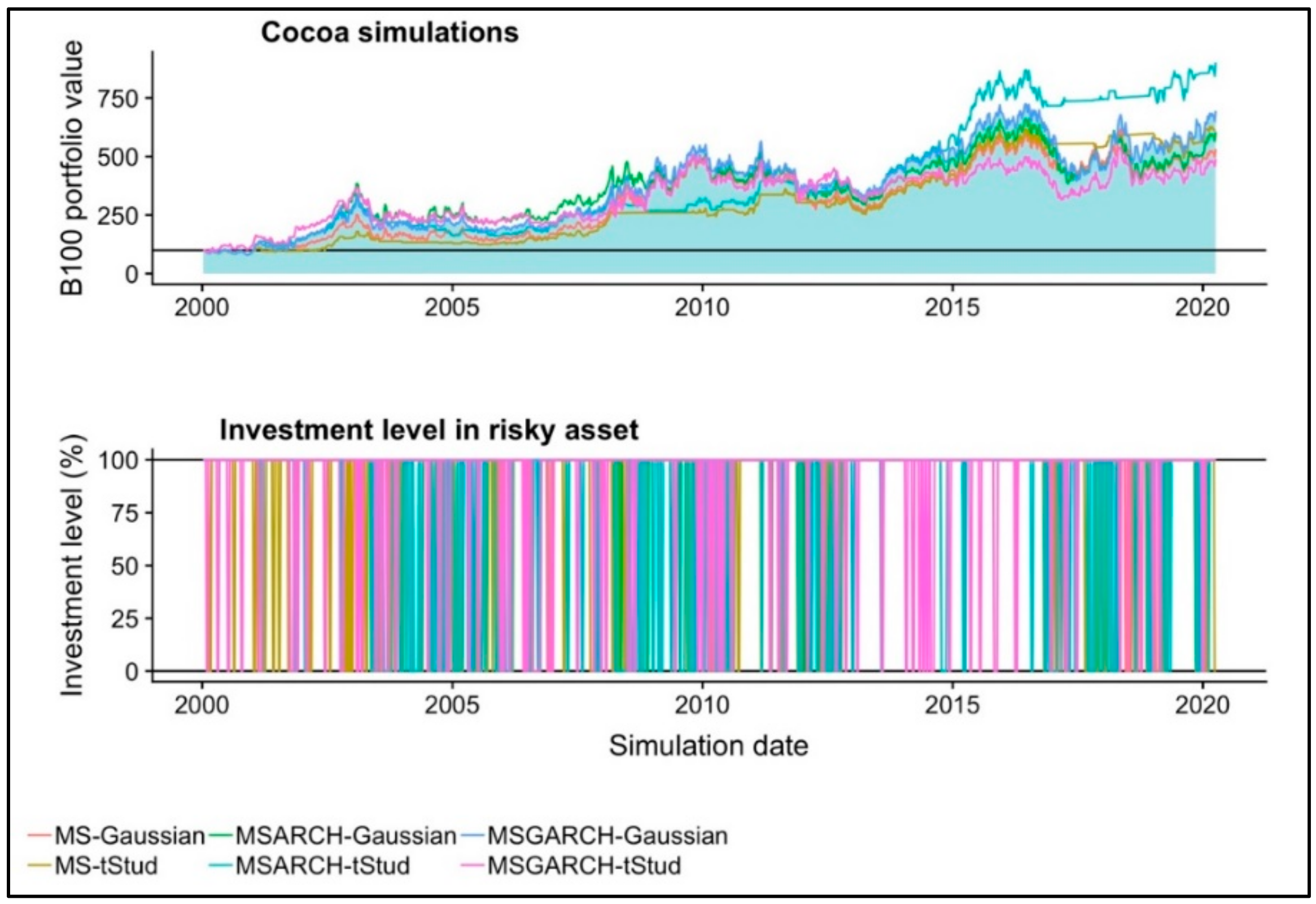
| Cocoa-MS-Gaussian | 431.843 | 0.1583 | 3.9399 | −14.1671 | 0.0325 |
| Cocoa-MS-t Student | 512.7569 | 0.1717 | 2.4549 | −9.5813 | 0.0307 |
| Cocoa-MSARCH-Gaussian | 504.4178 | 0.1704 | 4.062 | −23.0489 | 0.0377 |
| Cocoa-MSARCH-t Student | 801.2475 | 0.2082 | 2.8363 | −23.0475 | 0.0386 |
| Cocoa-MSGARCH-Gaussian | 594.5557 | 0.1835 | 4.301 | −23.0542 | 0.038 |
| Cocoa-MSGARCH-t Student | 389.2472 | 0.1504 | 3.9084 | −23.0339 | 0.0297 |
| Portfolio | Accumulated Return | Mean Return | Return Std. Dev. | Lowest Weekly Return | Sharpe Ratio |
|---|---|---|---|---|---|
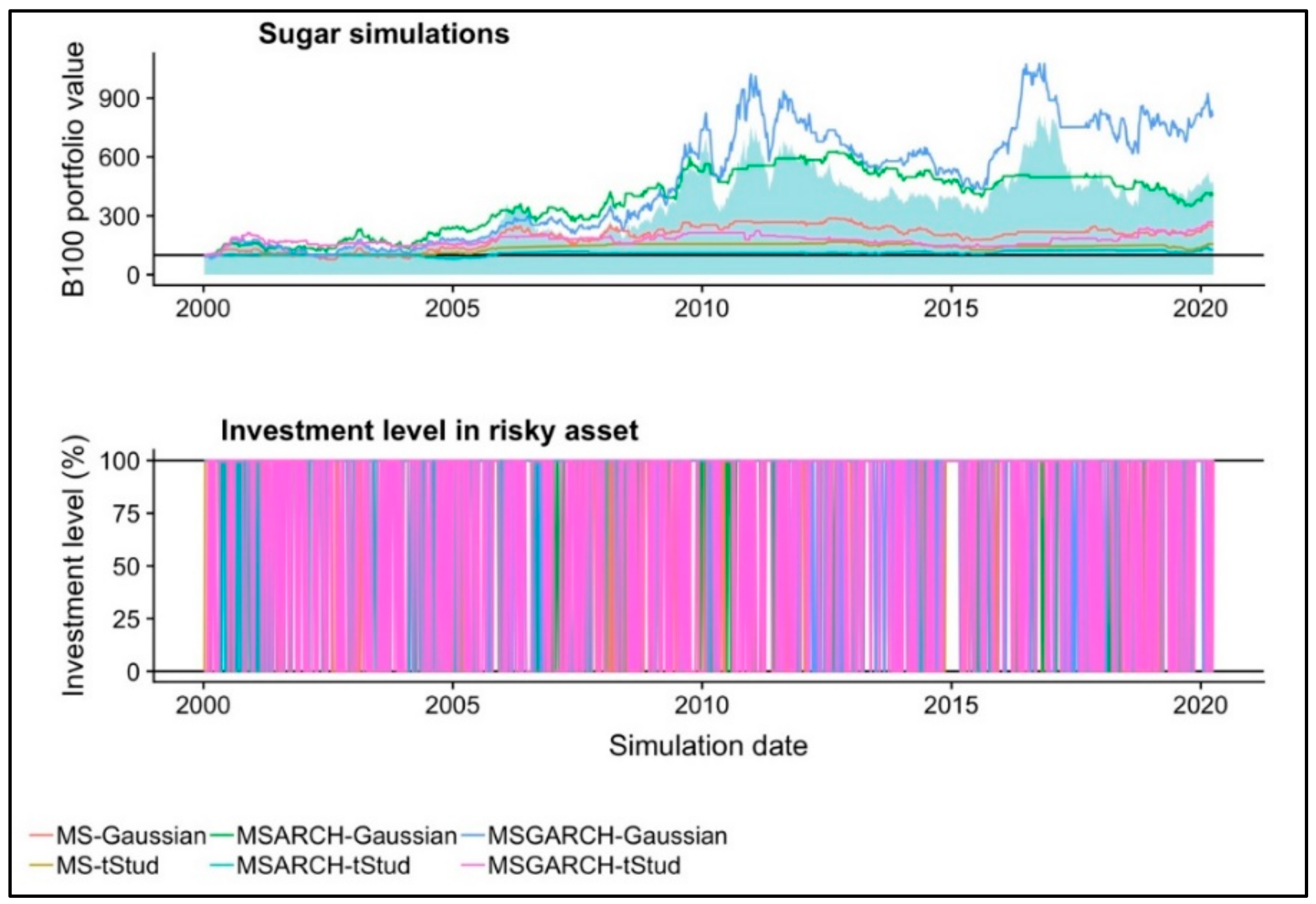
| Sugar-MS-Gaussian | 146.2971 | 0.0854 | 2.7338 | −12.6382 | 0.014 |
| Sugar-MS-tStud | 56.4792 | 0.0424 | 0.844 | −4.7119 | 0.0022 |
| Sugar-MSARCH-Gaussian | 306.4918 | 0.1328 | 2.7631 | −11.4508 | 0.0288 |
| Sugar-MSARCH-tStud | 27.1906 | 0.0228 | 0.9576 | −6.6802 | −0.0059 |
| Sugar-MSGARCH-Gaussian | 710.7164 | 0.1982 | 4.1223 | −17.3937 | 0.0348 |
| Sugar-MSGARCH-tStud | 167.8353 | 0.0933 | 2.1446 | −17.3852 | 0.0108 |
| Portfolio | Accumulated Return | Mean Return | Return Std. Dev. | Lowest Weekly Return | Sharpe Ratio |
|---|---|---|---|---|---|
| Coffee-MS-Gaussian | 11.3484 | 0.0102 | 4.0688 | −11.8899 | −0.0062 |
| Coffee-MS-tStud | 72.9009 | 0.0519 | 4.0685 | −11.8863 | −0.0003 |
| Coffee-MSARCH-Gaussian | 11.6724 | 0.0105 | 4.07 | −11.8899 | −0.0062 |
| Coffee-MSARCH-tStud | 4.2611 | 0.004 | 4.0444 | −11.8857 | −0.012 |
| Coffee-MSGARCH-Gaussian | 90.5161 | 0.061 | 4.1543 | −11.8899 | 0.0022 |
| Coffee-MSGARCH-tStud | −5.366 | −0.0052 | 3.8614 | −16.2139 | −0.0102 |
© 2020 by the authors. Licensee MDPI, Basel, Switzerland. This article is an open access article distributed under the terms and conditions of the Creative Commons Attribution (CC BY) license (http://creativecommons.org/licenses/by/4.0/).
Share and Cite
De la Torre-Torres, O.V.; Aguilasocho-Montoya, D.; del Río-Rama, M.d.l.C. A Two-Regime Markov-Switching GARCH Active Trading Algorithm for Coffee, Cocoa, and Sugar Futures. Mathematics 2020, 8, 1001. https://doi.org/10.3390/math8061001
De la Torre-Torres OV, Aguilasocho-Montoya D, del Río-Rama MdlC. A Two-Regime Markov-Switching GARCH Active Trading Algorithm for Coffee, Cocoa, and Sugar Futures. Mathematics. 2020; 8(6):1001. https://doi.org/10.3390/math8061001
Chicago/Turabian StyleDe la Torre-Torres, Oscar V., Dora Aguilasocho-Montoya, and María de la Cruz del Río-Rama. 2020. "A Two-Regime Markov-Switching GARCH Active Trading Algorithm for Coffee, Cocoa, and Sugar Futures" Mathematics 8, no. 6: 1001. https://doi.org/10.3390/math8061001
APA StyleDe la Torre-Torres, O. V., Aguilasocho-Montoya, D., & del Río-Rama, M. d. l. C. (2020). A Two-Regime Markov-Switching GARCH Active Trading Algorithm for Coffee, Cocoa, and Sugar Futures. Mathematics, 8(6), 1001. https://doi.org/10.3390/math8061001