Article

The Online Distribution System of Inventory-Routing Problem with Simultaneous Deliveries and Returns Concerning CO2 Emission Cost

1
Department of Information Management, Lunghwa University of Science and Technology, Taoyuan 33306, Taiwan
2
Department of Industrial Engineering and Enterprise Information, Tunghai University, Taichung 40704, Taiwan
3
Faculty of Finance and Banking, Ton Duc Thang University, Ho Chi Minh City 729000, Vietnam
*
Author to whom correspondence should be addressed.
Mathematics 2020, 8(6), 1002; https://doi.org/10.3390/math8061002
Submission received: 19 May 2020 / Revised: 14 June 2020 / Accepted: 15 June 2020 / Published: 18 June 2020

Abstract

:
This study attempts to consider CO2 emission cost to propose an online distribution system of inventory-routing problem with simultaneous deliveries and returns (IRPSDRCO2). The proposed IRPSDRCO2 mathematical models will be developed to find the total inventory routing cost, the CO2 emission cost, the optimal delivery routes, the economic order quantities, the optimal reordering points, the optimal service levels, the optimal common review interval, and the optimal maximum inventory levels for all retail stores delivered in these scheduled routes. The proposed IRPSDRCO2 model further applies the savings method, the target insert heuristic method, the target exchange heuristic method, and the repeated target heuristic method to find the optimal solution and the related scheduled routing plan. The sensitivity analyses will be conducted for this proposed IRPSDRCO2 model based on different parameters to provide very helpful decision-making information for a distribution system design. The performance of the proposed repeated target heuristic method is demonstrated to be better than most of four other combination methods regarding both the inventory routing cost and CPU running time. Consequently, it should be very helpful for logistics firms to design their distribution system by following the structure and the detailed procedure flow of the online distribution system developed by this study.

1. Introduction and Literature Review

Professional logistics companies in Taiwan usually deliver general products from depot to all retail stores by considering the trade-off relationship between transportation cost and inventory cost, which comprise the greatest part of total logistics cost. One of the well-known academic topics typically discussed in this field is the Inventory Routing Problem (IRP) [1,2,3,4,5,6,7,8,9]. Most IRP studies often apply transportation cost, holding cost, and ordering cost to design the related distribution system, but few of them use safety cost and shortage cost to conduct the routing plan. Reference [4] considers inventory holding cost, safety cost, shortage cost, ordering cost, and transportation cost to develop a decision support system of a green inventory-routing problem. Specifically, publishing products such as newspapers, magazines, books, greeting cards, and catalogs have the characteristic of a high return percentage [10]. The inventory-related costs are raised remarkably due to the return of out-of-date publishing products. Evidently, accurate forecasting of the merchandise and handling sales of out-of-date merchandise are very crucial. Unfortunately, these publishing logistics firms rarely consider the cost derived from returning out-of-date products back to depot and determine the delivered quantity of products for each retail store and the related vehicle delivery routes based on their past experiences. Accordingly, it is more appropriate to apply the academic field of the inventory-routing problem with simultaneous deliveries and returns (IRPSDR) to design the related distribution system.
Global warming is regarded as one of the most difficult concerns of this century. Thus, CO2 emission is gradually turning into the main concern for the whole world. Global warming mainly comes from increasing CO2 emission density in the atmosphere. To prevent global warming from becoming worse, several countries and organizations are complying with ‘green’ principles stipulated by the Kyoto Protocol, which took effect in 2005. Globalization, with its increasing industrial outsourcing needs, has resulted in transportation becoming the most important part that has strengthened CO2 emissions over the last two decades. In December 12 of 2015, nearly 200 nations completed the “Paris agreement” draft, which aims to keep global temperatures from rising another 2° Celsius until 2100 by eliminating greenhouse gas pollution. As a result, transportation operations play the major role of global warming, which leads to the latter dilatation of green logistics [11]. In Taiwan, transportation accounted close to 13.9% of the total CO2 emissions generated in 2011, of which CO2 emissions from road transport comprised approximately 94.7% [12,13]. In the academic field, there are some IRP studies discussing Greenhouse Gas (GHG) emission consumptions [4,11,14,15]. For a green IRP problem, Reference [15] analyzed the interests of horizontal collaboration regarding perishability, CO2 emissions from transportation activities, and logistics costs in the Inventory Routing Problem with numerous suppliers and customers by establishing a decision support model that can announce these concerns. Due to the enhancing environmental regard from the whole world, this paper intends to help logistics firms methodologically and practically design their distribution systems to include the produced CO2 emission cost into the objective function of the IRPSDR model, which becomes the IRPSDRCO2 model.
The development of Internet of Things (IoT) makes it possible to acquire a variety of real-time information. Real-time traffic and vehicle information based on IoT and mobile technology contribute to great significance on the vehicle routing planning. To optimize the routing planning of in-vehicle navigation with the help of IoT technology would decrease peoples’ travel cost, improve travel safety and satisfaction on the navigation system, and it would improve the city’s traffic condition globally. The vehicle routing problem (VRP) has always been the critical problem of traffic and navigation systems. Scholars have completed many studies about this topic [16,17,18,19,20,21,22]. According to our observations, most of them conduct the offline scheduled planning of the vehicle routing problem without considering instantaneous traffic congestion, which will cause more arrival time and fuel consumption. However, the recent development of IoT technology and the Internet of the vehicle would change the situation completely. This study tries to integrate mobile device, the Internet of the vehicle, and Google Map to enhance a traditional VRP navigation system into the online module of an IRPSDRCO2 related navigation system, which can also conduct the instantaneous routing plan to handle the real traffic situation and immediate customer’s requests. The IRPSDPCO2 developed by this study will first conduct scheduled vehicle routing planning and inventory control policy, which determine the optimal delivery routes, optimum review interval for all retail stores, and the related maximum level of products for each retail store located in those proposed routes based on the minimal total inventory routing cost criterion. Second, the instantaneous routing planning to handle the real traffic situation and immediate customer’s requests will be conducted with the help of an online in-vehicle navigation system.
This research employs specific Taiwan publishing logistics firm’s operating data to discuss its distribution system design problem. This study focuses on some specific logistics firms with a main distribution center, which deals with the distribution operation of publishing merchandise for many retail stores. However, it is not enough to only conduct re-ordering point inventory control policy in our proposed IRPSDPCO2 model. The main reason is that it has some economic disadvantages that the reorder point inventory control method conducts precise control over the inventory level of each merchandise item. For instance, each merchandise item is possibly ordered at a different time table and perhaps each retail store is also delivered at a different time table. Therefore, there are missing joint ordering, buying, or transportation economies. Furthermore, it will cause a lot of administrative difficulties in which the reordering point method requires constant monitoring of the inventory levels. Alternatively, under periodic review control, inventory levels for multiple merchandise items and different retail stores can be reviewed at the same time so that may be ordered and delivered at the same time, which realizes purchasing, production, or transportation economies. Compared to most of the previous existing IRP models, only applying reordering point inventory control policy to their methodological development, we will apply both the reordering point inventory control method and the periodic review inventory control method in our proposed IRPSDRCO2 model. Consequently, the inventory routing problem discussed in this research can be classified as two categories of reordering point inventory routing problem with simultaneous deliveries and returns concerning CO2 emission cost (ROPIRPSDRCO2) and periodic review inventory routing problem with simultaneous deliveries and returns concerning CO2 emission cost (PRIRPSDRCO2).
The IRPSDRCO2 proposed in this study is similar to a typical IRP problem, which is surely an NP-hard problem, and is not easy to manipulate by exact mathematical programming methods or simple heuristic approaches. The mathematical programming method can reach the optimal solution, but can only deal with a small-scale problem [6,7,15,18]. On the contrary, the simple heuristic approaches are normally applied to handle the large-scale NP-hard problem, but is frequently dropped into the local optimal solution [2,3,5,9]. Reference [3] studied a maritime IRP with time windows for deliveries with uncertain disruptions. A Lagrangian heuristic algorithm is proposed for acquiring flexible solutions by introducing auxiliary soft constraints incorporated in the objective function with Lagrange multipliers. Accordingly, meta-heuristic approaches have been employed to handle this type of difficult problem more efficiently to approach the optimal solution [1,7,8,21,23,24]. Reference [7] addressed a pickup and delivery inventory routing problem within time windows for a producer to distribute products packed in returnable transport items to a set of customers. A mixed-integer linear program is developed and tested on small-scale instances and a cluster first-route second meta-heuristic is proposed to handle more realistic large-scale problems. For decades to come, scholars have shown that the Tabu search (TS) method can deal with NP-hard problems such as VRP very efficiently. References [16,17,25] proposed a two-phase TS combined with the savings method [26] and a simple 2-opt procedure [27] for the solution of location and routing problem (LRP), which are significant improvements over heuristic methods comprising SAV1, SAV2, and CLUST algorithms from Reference [28]. For the location and inventory routing problem (LIRP), Reference [29] proposed a hybrid heuristic method merging TS and SA, which is much better than the heuristic method from Reference [30] and the SA method. Moreover, Reference [1] showed that the modified genetic algorithm (GA) surpasses two former heuristic approaches. Reference [23] conducted a predicting particle swarm optimization (PSO) algorithm to optimize the routing assignment problem. Reference [21] proved that the improved PSO algorithm performs well in solution accuracy, but the original PSO works better in computational time. Reference [8] presented the suggested Tabu heuristic method, which was better than the other two methods when considering the average profit. All above literatures clearly show that meta-heuristic methods such as TS, GA, SA, PSO, or the combination methods of meta-heuristic methods and simple heuristic approaches can achieve better performances in terms of VRP, LRP, and LIRP problems. Unfortunately, these meta-heuristic methods generally need plenty of computation time to near the optimal solution, and, therefore, are not appropriate to be applied in the online distribution system of IRPSDRCO2 developed in this study. Accordingly, this proposed IRPSDRCO2 mathematical model first conducts savings method to obtain the initial solution. Then, it conducts a target insert heuristic method, a target exchange heuristic method, and a repeated target heuristic method, which are further conducted to find the optimal solution and the related scheduled routing planning.

2. Problem Statement and Mathematical Model Formulation

2.1. Problem Statement and the Proposed Online Distribution System

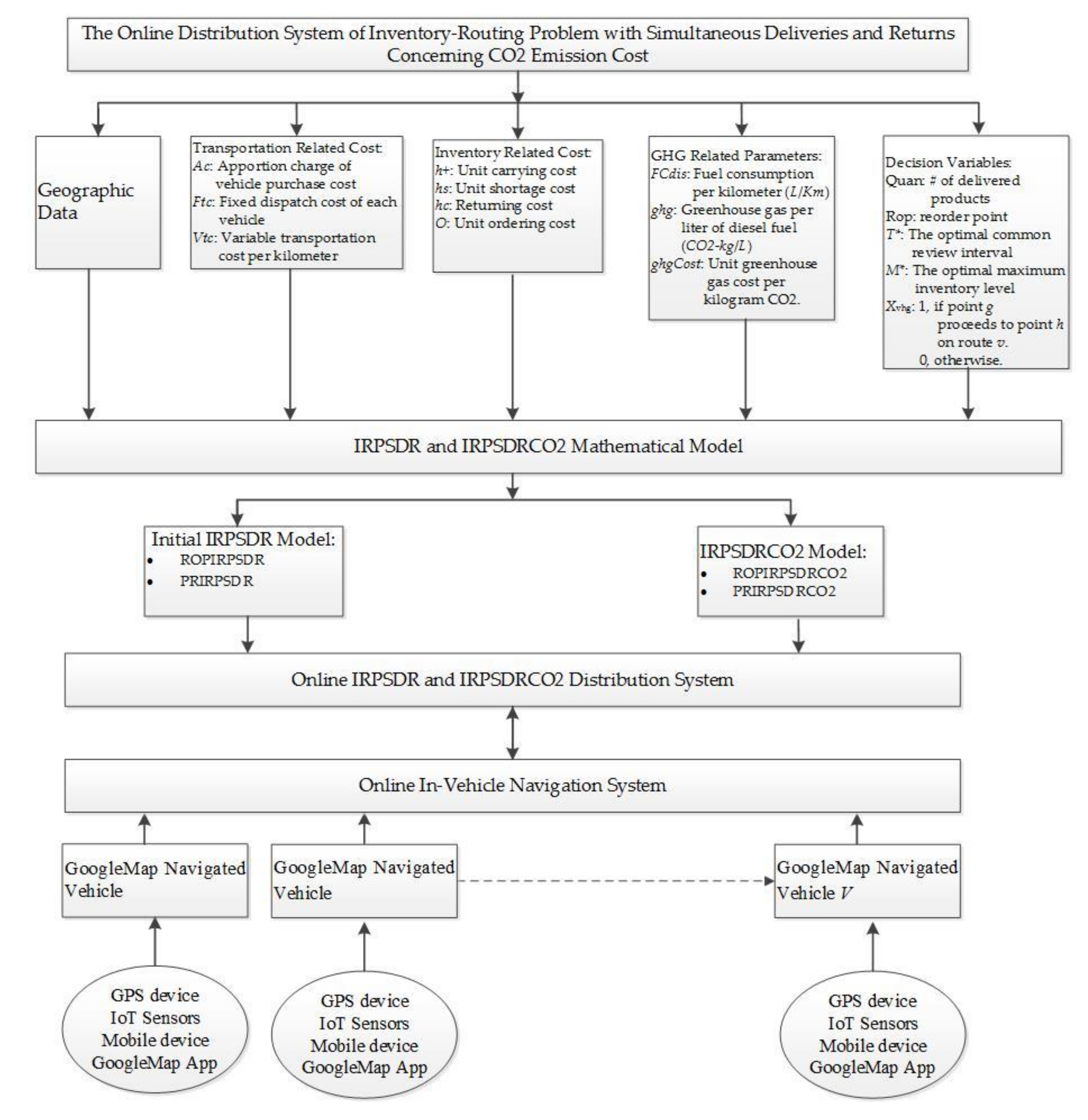
This paper primarily discusses the distribution operation of merchandise handled by some specific Taiwan logistics firm. This studied Taiwan logistics firm has a single main distribution center, which is in charge of the distribution operation for more than 5000 convenience retail stores, and delivers once a day and gets back the main distribution center after completing all deliveries of these retail stores. The proposed IRPSDRCO2 mathematical model will be developed to deal with the scheduled delivery of products to all retail stores and the return of out-of-date products back to the distribution center, but need to reduce the problem scope due to several research constraints. An online distribution system is further developed to integrate the mobile device, Internet of the vehicle, and Google Map to enhance an online IRPSDRCO2 related navigation system for the distribution center run by some specific logistics firm. The structure of our proposed online distribution system are shown in Figure 1.
The main structure of our proposed online distribution system shown in Figure 1 includes (1) IRPSDR and IRPSDRCO2 Mathematical Model, (2) online IRPSDR and IRPSDRCO2 distribution system, (3) Online In-Vehicle Navigation System, and (4) Google Map Navigated Vehicles Associated with GPS Devices, Mobile Devices, IoT Sensors, Google Map Apps.

2.2. Research Limitations and Assumptions

(1)
This study considers a general publishing merchandise and single-depot inventory-routing problem with simultaneous deliveries and returns.
(2)
The amount and location of the distribution center and retail stores are precisely acquired, and the actual distances of these stores are adopted in this study.
(3)
The travel time between two retail stores is fixed and depends on the actual distance between these two stores.
(4)
Each retail store is only delivered by one truck.
(5)
Each route is also only delivered by one truck.
(6)
All routes start and end at the same distribution center.
(7)
The distribution center will not be restricted by the product capacity.
(8)
The total demand of each route is less than or equal to the truck loading capacity.
(9)
This research concerns ordering cost, inventory carrying cost, transportation cost, shortage cost, and returning cost of each store.
(10)
The demand of each retail store is presumed to follow normal distribution or general distribution.
(11)
The reordering inventory control policy and the period review inventory control policy are discussed.
(12)
The types of all trucks are homogeneous Google Map navigated trucks associated with GPS devices, IoT sensors, mobile devices, and Google Map Apps.
(13)
The proposed online in-vehicle navigation system sets up the route sequence planned by the IRPSDRCO2 model and adopts Google Map navigated trucks to navigate and conduct delivery and return operations.

2.3. Notation

  • h, g, j: Index of retail stores and depot
  • i: Index of retail stores
  • v: Index of vehicles
Decision variables:
  • Q u a n v g h : Volume of products delivered each time from store g to store h by truck v.
  • R o p v g h : The inventory level of reorder point for h proceeded by g on route v.
  • T * : The optimal common review interval for all retail stores.
  • M i * : The optimal maximum inventory level for each retail store i.
  • X v g h : 1, if store g immediately proceeds to store h on route v (truck v).
  • 0, otherwise.
  • N: Amount of retail stores.
  • V: Amount of vehicles.
  • cap: Limit of vehicle loading capacity.
  • Ac: Apportion charge of vehicle purchase cost.
  • Ftc: Fixed dispatch cost of each vehicle.
  • Vtc: Variable transportation cost per kilometer.
  • h + : Unit carrying cost.
  • h s : Unit shortage cost.
  • h c : Returning cost.
  • O: Unit ordering cost.
  • F C d i s : Fuel consumption per kilometer (L/Km).
  • g h g : Greenhouse gas per liter of diesel fuel (CO2-kg/L).
  • g h g C o s t   : Unit greenhouse gas cost per kilogram CO2.
    LT: Lead time.
  • D e m v g h Total demand of products delivered within a period from store g to h by truck v.
  • d e m v g h : Demand of products delivered each day from store g to h by truck v.
  • L a d v g h The average demand of store h in route v during the lead time.
  • I n v v g h The inventory level of store h in route v in which the replenishment order is placed.
  • s d : Standard deviation of product demand per day.
  • s d : Standard deviation of product demand within the lead time ( s d = s d L T for ROPIRPSDR and ROPIRPSDRCO2, s d = s d L T + T * for PRIRPSDR and PRIRPSDRCO2).
  • D i s v g h : Delivered distance from store g to store h by vehicle v.
  • Y i j : 1 if retail store j is assigned to distribution center i, 0 otherwise.
  • u : One specific route in the proposed IRPSDRCO2 distribution system.
  • u ¯ : All other routes in the proposed IRPSDRCO2 distribution system.
    T_cost: Total inventory routing cost.

2.4. Mathematical Model Formulation

This study restricts the problem scope to one distribution center and around 5000 retail stores. The online IRPSDP and IRPSDPCO2 mathematical models applying reordering point inventory policy (ROPIRPSDR and ROPIRPSDRCO2) and period review inventory policy (PRIRPSDR and PRIRPSDRCO2) are developed to find the optimal scheduled delivery routes, the economic order quantities, the optimal reordering points, the optimal service levels, the optimal common review interval, and the optimal maximum inventory levels for all retail stores delivered in these proposed routes. These two proposed mathematical models are delineated as follows.
Minimize the following:
  • Case 1: IRPSDR Model
    v = 1 V g = 1 N + 1 h = 1 N + 1 ( Q u a n v g h 2 * h + + D e m v g h Q u a n v g h * O + ( R o p v g h L a d v g h ) * h + + D e m v g h Q u a n v g h * h s * B ( R o p v g h ) + D e m v g h Q u a n v g h * h c * C ( R o p v g h ) + D e m k g h Q u a n k g h * ( V t c * D i s v g h + F t c ) ) * X v g h + V * A c
  • Case 2: IRPSDRCO2 Model
    v = 1 V g = 1 N + 1 h = 1 N + 1 ( Q u a n v g h 2 * h + + D e m v g h Q u a n v g h * O + ( R o p v g h L a d v g h ) * h + + D e m v g h Q u a n v g h * h s * B ( R o p v g h ) + D e m v g h Q u a n v g h * h c * C ( R o p v g h ) + D e m k g h Q u a n k g h * ( V t c * D i s v g h + F t c + F C d i s * g h g * D i s k g h * g h g C o s t   ) ) * X v g h + V * A c
  • St: (both of Case 1 and Case 2)
    g = 1 N + 1 h = 1 N + 1 ( Q u a n v g h + C ( R O P v g h ) )   c a p ,        v = 1 , V
    v = 1 V h = 1 N + 1 X g v h = 1 ,        g = 1 , N
    g = 1 N + 1 X h g v g = 1 N + 1 X g h v = 0 ,     v = 1 , V , h = 1 , N + 1
    g = 1 N h = N + 1 N + 1 X g h v 1 , v = 1 , V
    h = 1 N + 1 X i h v + h = 1 N + 1 X j h v Y i j 1 , i = 1 , N , j = N + 1 , v = 1 , V
    g u h u ¯ v = 1 V X g h k 1 ,    ( u ,   u ¯ )
    X v g h = 0 ,    1 ,     g = 1 , N + 1 , h = 1 , N + 1 ,     v = 1 , V
    Y i j = 1 , i = 1 , N , j = N + 1
In the above mathematical model formulation, the objective function includes the inventory routing costs of all retail stores located in all delivered routes.
  • Case 1: IRPSDR Model
    v = 1 V g = 1 N + 1 h = 1 N + 1 ( Q u a n v g h 2 * h + + D e m v g h Q u a n v g h * O + ( R o p v g h L a d v g h ) * h + + D e m v g h Q u a n v g h * h s * B ( R o p v g h ) + D e m v g h Q u a n v g h * h c * C ( R o p v g h ) + D e m v g h Q u a n v g h * ( V t c * D i s v g h + F t c ) ) * X v g h , and the apportion charge of fixed vehicle purchase cost V * A c .
The inventory-routing cost between two delivered retail stores can be described as follows:
Q u a n v g h 2 * h + + D e m v g h Q u a n v g h * O + ( R o p v g h L a d v g h ) * h + + D e m v g h Q u a n v g h * h s * B ( R o p v g h ) + D e m v g h Q u a n v g h * h c * C ( R o p v g h ) + D e m v g h Q u a n v g h * ( V t c * D i s v g h + F t c )
  • Case 2: IRPSDRCO2 Model
    v = 1 V g = 1 N + 1 h = 1 N + 1 ( Q u a n v g h 2 * h + + D e m v g h Q u a n v g h * O + ( R o p v g h L a d v g h ) * h + + D e m v g h Q u a n v g h * h s * B ( R o p v g h ) + D e m v g h Q u a n v g h * h c * C ( R o p v g h ) + D e m v g h Q u a n v g h * ( V t c * D i s v g h + F t c ) + D e m k g h Q u a n k g h * ( F C d i s * g h g * D i s k g h * g h g C o s t   ) ) * X v g h , and the apportion charge of fixed vehicle purchase cost V * A c .
The inventory-routing cost between two delivered retail stores can be described as follows.
Q u a n v g h 2 * h + + D e m v g h Q u a n v g h * O + ( R o p v g h L a d v g h ) * h + + D e m v g h Q u a n v g h * h s * B ( R o p v g h ) + D e m v g h Q u a n v g h * h c * C ( R o p v g h ) + D e m v g h Q u a n v g h * ( V t c * D i s v g h + F t c ) + D e m k g h Q u a n k g h * ( F C d i s * g h g * D i s k g h * g h g C o s t )
The above cost includes the average inventory carrying cost, the ordering cost, the safety stock inventory carrying cost, the shortage cost, the returning cost, the transportation cost, and the greenhouse gas emission cost. They are described in detail as follows.
  • The average inventory carrying cost:   ( Q u a n v g h 2 ) * h +
  • The ordering cost:   D e m v g h Q u a n v g h * O
  • The safety stock inventory carrying cost:   ( R o p v g h L a d v g h ) * h +
  • The shortage cost:   D e m v g h Q u a n v g h * h s * B ( R o p v g h ) , where B ( R o p v g h ) = R o p v g h ( x R o p v g h ) f L ( x ) d x
  • The returning cost:   D e m v g h Q u a n v g h * h c * C ( R o p v g h ) , where C ( R o p v g h ) = 0 R o p v g h     ( R o p v g h x ) f L ( x ) d x
  • The transportation cost: D e m v g h Q u a n v g h * ( V t c * D i s v g h + F t c )
  • The greenhouse gas emission cost: D e m k g h Q u a n k g h * ( F C d i s * g h g * D i s k g h * g h g C o s t   )
In the above constraint functions, constraint (1) indicates that the quantity of each delivery to retail stores and the quantity of each return back to the distribution center must be less than or equal to vehicle loading capacity. Constraint (2) expresses that each customer can only appear in one route. Constraint (3) implies that each store entered by the truck should be the same store the truck leaves. Constraint (4) means a route can only be served by one distribution center. Constraint (5) denotes that a retail store can be assigned to a distribution center only if there is a route passing by that retail store. Constraint (6) states that each route begins and ends at the same distribution center. Constraints (7) and (8) represent the integrality of decision variables.

2.5. The Procedure Flow of the Online IRPSDRCO2 Distribution System

The main procedure of our proposed online distribution system is as follows.
Step 1Model Development: (1) Develop the simulated IRPSDR mathematical models including ROPIRPSDR, PRIRPSDR, ROPIRPSDRCO2, and PRIRPSDRCO2. (2) Develop routing algorithms including a saving method, a target insert heuristic method, a target exchange heuristic method, and a repeated target heuristic method. (3) Develop the simulation cases regarding to different parameters including truck type, inventory carrying cost percentage, unit shortage cost, unit return cost, unit ordering cost, and unit transport cost. Step 2 Manipulation Process: (1) Input the relevant inventory routing information and CO2 information. (2) Obtain the Initial solution by conducting the saving method. (3) Improve the initial solution to approximate to the optimal solution by implementing the target insert heuristic method, target exchange heuristic method, and repeated target heuristic method. Step 3 Simulated Results Analysis: (1) Illustrate the simulated results including the optimum total inventory routing cost, the optimum scheduled delivery routes, and the economic order quantities, the optimum service levels, the reorder points, the optimum common review interval, and the optimum maximum inventory levels of all retail stores in these planned routes. (2) Conduct the sensitive analyses regarding different parameters including truck type, inventory carrying cost percentage, unit shortage cost, unit return cost, unit ordering cost, and unit transport cost. Step 4 Design the Delivered Routes: Visualizes and displays the planned online IRPSDR or IRPSDRCO2 distribution system design. Step 5 Conduct the Delivery and Return Operation: Applies online in-vehicle navigation system to conduct the delivery and return operations according to the scheduled routes planned by the online IRPSDR or IRPSDRCO2 distribution system.
The detailed procedure flow of our proposed online distribution system are shown in Figure 2.

3. The Proposed Target Heuristic Methods

This research applies the savings method [26] and three proposed target heuristic methods including the target insert heuristic method, the target exchange heuristic method, and the repeated target heuristic method are conducted to solve the proposed IRPSDRCO2 model. First, in the first phase, the savings method is used to get the initial feasible solution. Moreover, in the second phase, the target insert heuristic method, target exchange heuristic method, and repeated target heuristic method are further conducted to find the optimal solution and the related scheduled routing planning. The detailed procedures of these proposed routing algorithms are delineated as follows.
Phase 1:
Obtain the initial solution by conducting the savings method.
Step 1:
Constitute the actual distances within all stores including one distribution center and all retail stores.
Step 2:
Constitute the initial values of parameters including cap, Ac, Ftc, Vtc, h + , h s , h c , O, LT, D e m k g h , dem, s d , F C d i s , g h g , g h g C o s t   .
Step 3:
Conduct the savings method (from Step 4 to Step 9). The pair of retail stores with the largest savings value is picked to the route.
Step 4:
Randomly choose one retail store j1, and then select the next transit retail store to put in any position of the original route based on the total inventory routing cost, T_cost. The calculation procedure of T_cost is deducted in the following Step 5, Step 6, and Step 7.
Step 5:
Compared to the VRP model, which adopts the actual distances within all stores including one distribution center and all retail stores to manipulate the optimal routing solution, our proposed IRPSDRCO2 applies inventory routing cost within all stores to find the optimal solution instead. The procedure to obtain the optimal inventory routing cost within all stores is described in the following steps. The optimal economic order quantity Q * , the optimal service level P * , and the optimal reorder point R o p * for all retail stores can also be acquired simultaneously.
The reordering point inventory policy is applied in the following steps. The demand of all retail stores follow general distribution including normal distribution.
Step (1):
Find the optimal delivered quantity and reorder point by first applying the reorder point inventory model.
The optimum delivered quantity and optimum reorder point can be obtained by presuming the first derivative of Equation (9) of case 1 and Equation (10) of case 2 equal to 0.
First, by presuming the first derivative of Equation (9) in Q u a n k g h equal to 0 for case 1 and the first derivative of Equation (10) in Q u a n k g h equal to 0 for case 2, it leads to:
Case 1: IRPSDR Model
  h + 2 D e m k g h Q u a n k g h 2 * O D e m k g h Q u a n k g h 2 * h s * B ( R o p k g h ) D e m k g h Q u a n k g h 2 * h c * C ( R o p k g h )   D e m k g h Q u a n k g h 2 * ( V t c * D i s k g h + F t c ) = 0       Q u a n k g h * = 2 D e m k g h ( O + h s * B ( R o p k g h ) + h c * C ( R o p k g h ) + F t c + V t c * D i s k g h   ) h +
Case 2: IRPSDRCO2 Model
  h + 2 D e m k g h Q u a n k g h 2 * O D e m k g h Q u a n k g h 2 * h s * B ( R o p k g h ) D e m k g h Q u a n k g h 2 * h c * C ( R o p k g h )   D e m k g h Q u a n k g h 2 * ( V t c * D i s k g h + F t c ) D e m k g h Q u a n k g h 2 * ( F C d i s * g h g * D i s k g h * g h g C o s t   ) = 0       Q u a n k g h * = 2 D e m k g h ( O + h s * B ( R o p k g h ) + h c * C ( R o p k g h ) + F t c + V t c * D i s k g h + F C d i s * g h g * D i s k g h * g h g C o s t   ) h +
By supposing the first derivative of Equation (9) in R o p k g h equal to 0 and the first derivative of Equation (10) in R o p k g h equal to 0, it results in both case 1 and case 2 as follows.
h + + h s * D e m k g h Q u a n k g h * d B ( R o p k g h ) d R o p k g h + h c * D e m k g h Q u a n k g h * d C ( R o p k g h ) d R o p k g h = 0      F L ( R o p k g h ) = h s h s + h c h + Q k g h ( h s + h c ) D k g h
Step (2):
Approximate the initial order quantity from the modified Economic Order Quantity (EOQ) formula.
Case 1: IRPSDR Model
Q u a n k g h = 2 D e m * ( O + F t c + V t c * D i s k g h ) h +
Case 2: IRPSDRCO2 Model
Q u a n k g h = 2 D e m * ( O + F t c + V t c * D i s k g h + F C d i s * g h g * D i s k g h * g h g C o s t   ) h +
Step (3):
Substitute Q u a n k g h of (14) in case 1 or Q u a n k g h of (15) in case 2 into Equation (13) to obtain the revised R o p k g h , respectively.
Step (4):
Substitute the revised R o p k g h obtained in Step (3) into Equation (11) in case 1 or Equation (12) in case 2 to find the revised Q u a n k g h , respectively.
Step (5):
Substitute the revised Q u a n k g h obtained in Step (4) into Equation (13) to determine the revised R o p k g h .
Step (6):
Repeat Step (4) and Step (5) until there is no more change in R o p k g h * and Q u a n k g h * .
Step (7):
Q u a n v g h * of all retail stores given in Step (6) are applied to obtain the optimal common review interval for all retail stores.
T * = i = 1 N Q u a n i * d e m i N
Step (8):
Apply R o p v g h * of all retail stores given in Step (6) and T * given in Step (7) to find the optimum maximum inventory level for each store i.
M i * = d e m i ( T * + L T ) + ( R o p i L a d i )
Step 6:
Calculate service level P k g h * = F L ( R o p * k g h ) , and other statistics related to the above converged R o p k g h * and Q u a n k g h * .
Step 7:
Acquire T_cost (j1+j2) by inputting the final converged P k g h * , Q u a n k g h * , R o p k g h * , and the related statistics of all paired points to the following formula.
  • Case 1: IRPSDR Model
  • ROPIRPSDR mode:
    ( Q u a n k g h * 2 ) * h + + D e m k g h Q u a n k g h * * O + ( R o p k g h * L a d k g h ) * h + + D e m k g h Q u a n k g h * * h s * B ( R o p k g h * ) + ( D e m v g h Q u a n v g h * h c * C ( R o p k g h * ) + D e m k g h Q u a n k g h * * ( V t c * D i s k g h + F t c )
  • PRIRPSDR mode:
    ( Q u a n k g h * 2 ) * h + + D e m k g h Q u a n k g h * * O + ( R o p k g h L a d k g h ) * h + + D e m k g h Q u a n k g h * * h s * B ( R o p k g h ) + ( D e m v g h Q u a n v g h * h c * C ( R o p k g h ) + D e m k g h Q u a n k g h * * ( V t c * D i s k g h + F t c )
    where ROP’ = d e m * ( L T + T * / 2 ) + s d * L T + T * * Z P *
  • Case 2: IRPSDRCO2 Model
  • ROPIRPSDRCO2 mode:
    ( Q u a n k g h * 2 ) * h + + D e m k g h Q u a n k g h * * O + ( R o p k g h * L a d k g h ) * h + + D e m k g h Q u a n k g h * * h s * B ( R o p k g h * ) + ( D e m v g h Q u a n v g h * h c * C ( R o p k g h * ) + D e m k g h Q u a n k g h * * ( V t c * D i s k g h + F t c ) + D e m k g h Q u a n k g h * ( F C d i s * g h g * D i s k g h * g h g C o s t   )
  • PRIRPSDRCO2 mode:
    ( Q u a n k g h * 2 ) * h + + D e m k g h Q u a n k g h * * O + ( R o p k g h L a d k g h ) * h + + D e m k g h Q u a n k g h * * h s * B ( R o p k g h ) + ( D e m v g h Q u a n v g h * h c * C ( R o p k g h ) + D e m k g h Q u a n k g h * * ( V t c * D i s k g h + F t c ) + D e m k g h Q u a n k g h * ( F C d i s * g h g * D i s k g h * g h g Cos t   )
    where ROP’ = d e m * ( L T + T * / 2 ) + s d * L T + T * * Z P *
Calculate the difference value dif = T_cost (j1+j2) – T_cost (j1) for all candidates of next transit retail stores. Choose the next transit retail store j2 with the smallest difference value and check if total demand by adding j2 to the route, which, when the truck is loaded, is less than or equal to the truck loading capacity. If it is, retail store j2 will be put into the route and marked. If it is not, reject j2 and choose another retail store with the next smallest difference value to check it again. Repeat the above procedure until, eventually, you find the next transit retail store.
Step 8:
Repeat Step 4, Step 5, Step 6, and Step 7 to choose the retail stores yet marked to be included in the route until the loading capacity of the truck delivered for the route is full.
Step 9:
If there are still retail stores unselected, go back to Step 3. If not, directly proceed to Step 10.
Step 10:
Record the current optimal solution including delivery routes, the objective function value, and the related decision variables to be the initial solution of phase 2.
Step 11:
Stop.
  • Phase 2: Improve the initial solution
After acquiring the initial total inventory routing cost in phase 1, we first conduct the target insert heuristic method to improve the initial total inventory routing cost. Next, the target exchange heuristic method is applied to ameliorate the current best total inventory routing cost. Lastly, we continue to advance the current best T_cost by conducting the repeated target heuristic method, which duplicates the target insert heuristic method and target exchange heuristic method alternatively until no further improvement of T_cost has been done. The detailed procedures of the target insert heuristic method, target exchange heuristic method, and repeated target heuristic method in phase 2 are described as follows.
Target insert heuristic method:
Step 1:
Set up the solution obtained in Phase 1 to be the initial solution of Phase 2.
Step 2:
Assign the last route planned in Phase 1 as the target insert route to implement the target insert heuristic method.
Step 3:
Calculate the objective function value by inserting all points located in all other routes into all possible positions between two points in the target route and check if it is possible to improve the initial solution obtained in phase 1 under the situation that the total amounts of delivered products of all retail stores originally in the target insert route plus the new inserted point from other routes is less than or equal to truck loading capacity. If yes, proceed to step 4. Otherwise, proceed to step 5.
Step 4:
Record all improved insert moves as the candidate list. Choose the insert move with the lowest objective function value from the candidate list and update the planned routes to deliver products to retail stores and return products to the distribution center. Return to step 3.
Step 5:
Stop.
Target exchange heuristic method
Step 1:
Set up the solution obtained from the target insert heuristic method to be the initial solution of the target exchange heuristic method.
Step 2:
Appoint the last route planned by the target insert heuristic method as the target exchange route to run the target exchange heuristic method.
Step 3:
Calculate the objective function value by exchanging all points located in all other routes with all possible points located in the target route and check if it is possible to improve the objective function solution obtained by the target insert heuristic method under the situation that the total amount of delivered products of all retail stores in the target exchange route and the total amount of delivered products of all retail stores in the selected exchange route are less than or equal to vehicle loading capacity. If yes, go to step 4. Otherwise, go to step 5.
Step 4:
Record all improved exchange moves as the candidate list. Choose the exchange move with the lowest objective function value from the candidate list and update the planned routes to deliver products to retail stores and return products to the depot. Return to step 3.
Step 5:
Stop.
Repeated target heuristic method:
Step 1:
Set up Ite to be the number of iterations of non-improved target moves. Set up Max_Ite to be the defined threshold of iteration of non-improving target moves.
Step 2:
Conduct the target insert heuristic method and target exchange heuristic method alternatively to improve the current lowest objective function value.
Step 3:
If the objective function value is improved, go back to step 2, or set up Ite=Ite+1. Go to step 4.
Step 4:
If Ite <= Max_Ite, go back step 2, or go to step 5.
Step 5:
Stop.

4. Simulated Numerical Results and Comparisons

In the following simulation study cases, the targeted publishing logistics firm has only one distribution center, which ships different merchandise to no less than 5000 convenience retail stores once a day. Due to the complexity of real logistics operation realized by this distribution center, the problem will be too complicated to study if the complete procedure of a real operation is directly adopted to demonstrate these proposed target heuristic methods. This research picked all delivered convenience stores of 10 routes located at the high-density region of population plus the distribution depot to be the research targeted area. The complete manipulating data and parameters are given based on the typical operating activities of this simulation case.
(1)
The average values and standard deviations of all 418 convenience stores are calculated based on the actual demands of the retail stores gathered by this study.
(2)
The lead time is estimated to be one day.
(3)
The price per unit of general merchandise is estimated to be 98 NT dollars.
(4)
The carrying cost is presumed to be 20% of the merchandise’s price.
(5)
The ordering cost is assumed to be 100 NT dollars per order.
(6)
h s equals 20 NT dollars.
(7)
h c equals 5 NT dollars.
(8)
The 3.5-ton truck loading capacity is supposed to be around 3000 units of general merchandise, 7.8-ton truck loading capacity is around 6686 units of general merchandise, and an 11-ton truck loading capacity is around 9429 units of general merchandise.
(9)
Apportion charge of fixed truck purchase cost Ac is predicted to be around 16,659 NT dollars by allocating the truck purchase cost to a 3-month period,
(10)
Ftcs equals 30 NT dollars by allocating driver’s salary to each retail store of the proposed delivered route.
(11)
Vtc equals 3.9 NT dollars according to the average diesel fuel consumption.
(12)
Greenhouse gas emission parameters for various truck types are described in Table 1.

4.1. The Simulated Results for the IRPSDR Model

In this proposed simulation case, the IRPSDR model with the ROP mode (ROPIRPSDR) will be applied in the first replenishment run to deliver products to all retail stores. For the remaining replenishment runs, the IRPSDR model with a PR mode (PRIRPSDR) will be conducted to deliver products to all retail stores.
First, the total inventory routing costs for the proposed IRPSDR model with the ROP mode based on the above default operating data and parameters by conducting the savings method, target insert heuristic method, target exchange heuristic method, and repeated target heuristic method are illustrated in Table 2.
According to Table 2, the lowest total inventory routing cost 3,070,733 NT dollars is acquired by the proposed repeated target heuristic method. Since the lowest total inventory routing cost comes from the IRPSDR model with an ROP mode by implementing the proposed method, it can then decide the optimum delivery routes, economic order quantities, the optimum service levels, and the reorder points of all retail stores placed in these planed routes. From the point of view of decision making on this proposed inventory routing problem, the above result means that the decision makers should first deliver all products through eight planned optimal delivery routes to all retail stores, which conduct the related reordering inventory control policies. Table 3 shows the detailed route sequence for the first and last route of the eight delivery routes.
The following Table 4 presents the economic order quantities, optimum reorder points, and optimum service levels of all retail stores placed in Route 1 based on the derived reordering inventory control policy obtained in this simulation case.
By first conducting the IRPSDR model with the ROP mode, the reorder point method adopts precise control over each merchandise item in inventory at each retail store. Except the first replenishment and delivery run, most retail stores will definitely be delivered at different time schedules for the remaining replenishment and delivery runs. Therefore, it misses joint ordering, transporting, or buying economies. Alternatively, under periodic review control, inventory levels for multiple merchandise items and different retail stores can be reviewed at the same time so that these merchandise items may be ordered and delivered at the same time. Thus, this realizes production, transportation, or purchasing economies. Therefore, the IRPSDR model with the PR mode will be applied after the first delivery run for this simulation case. According to the results of Table 5, the total inventory routing cost for conducting the IRPSDR model with the PR mode by running the proposed repeated target heuristic method is 4,098,427 NT dollars, which is clearly higher than the lowest total inventory routing cost of 3,070,733 NT dollars obtained by the IRPSDR model with the ROP mode.
Moreover, the modified route sequences, the optimal common review interval, and optimal maximum inventory levels of all retail stores placed in these designed routes will be obtained in the sequel in Table 6 and Table 7.

4.2. The Simulated Results for IRPSDRCO2 Model

In this proposed simulation case, the IRPSDRCO2 model with the ROP mode (ROPIRPSDRCO2) will be applied in the first replenishment run to deliver products to all retail stores. For the remaining replenishment runs, the IRPSDRCO2 model with the PR mode (PRIRPSDRCO2) will be conducted to deliver products to all retail stores.
First, the total inventory routing costs for the proposed ROPIRPSDRCO2 based on the above default operating data and parameters by conducting the savings method, target insert heuristic method, target exchange heuristic method, and repeated target heuristic method are illustrated in Table 8.
With regard to Table 8, the repeated target heuristic method obtained the lowest total inventory routing cost of 3,145,568 NT dollars. Due to the lowest total inventory routing cost coming from the IRPSDRCO2 model with ROP mode, it can then determine the optimum delivery routes, and economic order quantities, the optimum service levels, and the reorder points of all retail stores placed in these scheduled routes. From the perspective of decision making on this proposed inventory routing problem, the above result means that the decision makers should first deliver all products through eight planned optimal delivery routes to all retail stores, which carry out the related reordering inventory control policies. Table 9 displays the detailed route sequence for the first and last route of the eight planned delivery routes.
Table 10 presents the optimum service levels, optimum reorder points, and economic order quantities of all retail stores placed in Route 1 based on the derived reordering inventory control policy obtained in this simulation case.
By first conducting the IRPSDRCO2 model with the ROP mode, the reorder point method applies precise control over each merchandise item at an inventory level at each retail store. Except the first replenishment and delivery run, most retail stores will deliver at different time tables for the remaining replenishment and delivery runs, and, therefore, will miss joint ordering, transporting, or buying economies. Alternatively, under periodic review control, inventory levels for multiple merchandise items and different retail stores can be reviewed at the same time so that these merchandise items may be ordered and delivered at the same time, which will help achieve production, transportation, or purchasing economies. Accordingly, the IRPSDRCO2 model with the PR mode will be conducted after the first delivery run for this simulated case. Regarding Table 11, the total inventory routing cost for implementing the IRPSDRCO2 model using the PR mode by running the proposed repeated target heuristic method is 4,098,427 NT dollars, which is clearly higher than the lowest total inventory routing cost of 3,145,568 NT dollars acquired by the IRPSDRCO2 model with the ROP mode.
Furthermore, the modified route sequences, the optimal common review interval, and optimal maximum inventory levels of all retail stores located in these designed routes will be demonstrated in the sequel in Table 12 and Table 13.

4.3. The Sensitivity Analysis for Decision Making Based on Different Parameters of IRPSDRCO2 with ROP Mode

The sensitivity analyses will be conducted for IRPSDRCO2 with the ROP mode based on different parameters including truck loading capacity, inventory carrying cost percentage, unit shortage cost, unit returning cost, unit ordering cost, and unit transport cost to provide very helpful decision-making information for IRPSDRCO2 system design.

4.3.1. The Sensitivity Analysis for Unit Shortage Cost Regarding ROPIRPSDRCO2 Mode

In Table 14, the sensitivity analysis of the proposed IRPSDRCO2 model with the ROP mode is conducted by altering the value of unit shortage cost including 17, 20, and 30 NT dollars.
According to Table 14, when the unit shortage cost is rising, it is shown to apply higher economical order quantity and follow the EOQ formula mechanism in Equation (12). It is cost-effective to conduct the optimal inventory control policy with a higher customer service level and ROP to avoid the stock-out situation.
The inventory cost is enlarged because of higher economical order quantity and the safety cost is increased due to a higher ROP level. Moreover, higher economical order quantity will lead to less delivery runs, and further cause lower transport cost, CO2 cost, and order cost. Although unit shortage cost is increased, higher economical order quantity will cause less delivery runs and further lead to lower shortage cost in these three specific numerical cases. The return cost is increased when unit shortage cost is increased in spite of the fact that higher economical order quantity will cause less delivery runs. The main reason is that the optimal inventory control policy of higher customer service level and higher reorder point will bring about more return products in these three given numerical cases.

4.3.2. The Sensitivity Analysis for Unit Return Cost Regarding the ROPIRPSDRCO2 Mode

In Table 15, the sensitivity analysis of the proposed IRPSDRCO2 model with the ROP mode is conducted by changing the value of unit return cost including 2, 5, and 8 NT dollars.
In the light of Table 15, when the unit return cost is rising, it directly gives rise to higher economical order quantity derived by the EOQ formula in Equation (12). It is profitable to apply a lower customer service level and reorder point to prevent the returning good situation.
It is certain that the inventory cost is increased because of higher economical order quantity applied and the safety cost is decreased due to lower ROP level conducted. Furthermore, higher economical order quantity will cause less delivery runs, and even cause lower transport cost, CO2 cost, and order cost. Although unit return cost is increased, higher economical order quantity causes less delivery runs but still leads to higher shortage cost due to optimal inventory control policy of a lower customer service level.
Lastly, the return cost is increased as a result of increased unit shortage cost in spite of the fact that the optimal inventory control policy of a lower customer service level and lower reorder point will bring about less return products.

4.3.3. The Sensitivity Analysis for Inventory Carrying Cost Percentage Regarding ROPIRPSDRCO2 Mode

In Table 16, the sensitivity analysis of the proposed IRPSDRCO2 model with the ROP mode is conducted by changing the value of inventory carrying cost percentage including 0.1, 0.2, and 0.3 NT dollars.
In line with Table 16, when the inventory carrying cost percentage is growing, it leads to increasing inventory carrying cost and small economical order quantity obtained by EOQ Equation (12). Therefore, tiny economical order quantity will cause more delivery runs, and further result in higher transport cost, order cost, and CO2 cost. It is also demonstrated that the proposed optimal inventory control policy adopts a low level of customer service and reorder point in order to refrain the high inventory carrying cost due to an increasing inventory carrying cost percentage. In addition, when the inventory carrying cost percentage is growing, more delivery runs, a low level of customer service, and reorder point will cause a higher shortage cost.
Table 16 also shows that the return cost is still increased even the growing inventory carrying cost percentage leads to the optimal inventory control policy, which implements the lower customer service level to reduce the amount of returning products. The main reason is that the increased effect of return cost caused by more delivery runs exceeds the decreased effect of return cost derived by the optimal inventory control policy to conduct a lower customer service level in these numerical cases. The safety inventory carrying cost is increased with a growing inventory carrying cost percentage because the increased effect of safety inventory carrying cost resulted in an increased inventory carrying cost percentage surpassing the decreased effect of safety inventory carrying cost incited by a smaller ROP.

4.3.4. The Sensitivity Analysis for Unit Order Cost Regarding ROPIRPSDRCO2 Mode

In Table 17, the sensitivity analysis of the proposed IRPSDRCO2 model with the ROP mode is conducted by changing the value of the unit order cost including 50, 100, and 150 NT dollars.
With regard to Table 17, when the unit order cost is increasing, it directly leads to large economical order quantity derived by the EOQ formula in Equation (12) and further creates raising inventory carrying cost. A larger economical order quantity will cause less delivery runs and lower return cost and CO2 cost. It is also demonstrated that, in these three specific numerical cases, the proposed optimal inventory control policy adopts a low level of customer service and reorder point in order to refrain the high inventory carrying cost due to large economical order quantity. Moreover, the shortage cost is increased because the increased effect of shortage cost resulted in a low level of customer service and the reorder point surpasses the decreased effect of shortage cost created by fewer delivery runs.

4.3.5. The Sensitivity Analysis for Variable Transport Cost Regarding ROPIRPSDRCO2 Mode

In Table 18, the sensitivity analysis of the proposed IRPSDRCO2 model with the ROP mode is conducted by changing the value of variable transport cost comprising 3, 3.9, and 6 NT dollars.
In Table 18, when the variable transport cost is enhancing, it undoubtedly derives bigger economical order quantity obtained by the EOQ Equation (12) and generates raising inventory carrying cost. A bigger economical order quantity will result in few delivery runs and still bring about less order cost and CO2 cost.
It is also illustrated that the recommended optimal inventory control policies in these three specific numerical cases adopt an increasing level of customer service and reorder point, which certainly causes more safety cost. Moreover, the shortage cost is decreased because of less delivery runs and an increasing level of customer service and reorder point.
In these three specific numerical examples, the transport cost is increased because the increased effect of transport cost created by increased variable transport cost exceeds the declined effect of transport cost caused by fewer delivery runs. The return cost is decreased because the dropping influence of return cost made by fewer delivery runs transcends the consequence of more return products aroused by an increasing level of customer service and reorder point.

4.3.6. The Sensitivity Analysis for Unit CO2 Cost Regarding ROPIRPSDRCO2 Mode

In Table 19, the sensitivity analysis of the proposed IRPSDRCO2 model with ROP mode is carried out by modifying the value of unit CO2 cost consisting of 35, 40, and 50 NT dollars.
According to the above results in Table 19, while the unit CO2 cost is growing, it spurs great economical order quantity acquired by the EOQ Equation (12) and generates rising inventory carrying cost. Moreover, great economical order quantity will lead to few delivery runs and give rise to less transport cost and order cost.
The suggested optimal inventory control policies in the above three specific numerical examples apply a decreasing level of customer service and reorder point, which cause less safety cost.
In the above three specific numerical cases, the CO2 cost is increasing. The increasing effect of CO2 cost generated by a growing unit CO2 cost outpaces the declining effect of CO2 cost caused by fewer delivery runs. On the contrary, the conflicting effect between fewer delivery runs and a decreasing level of customer level and reorder point leads to unclear ascending or descending trend of shortage cost.

4.3.7. The Sensitivity Analysis for Truck Loading Capacity Regarding ROPIRPSDRCO2 Mode

In Table 20, the sensitivity analysis of the proposed IRPSDRCO2 model with ROP mode is carried out based on three different truck loading capacity given by a 3.5-ton truck, a 7.8-ton truck, and an 11-ton truck.
Regarding the above results of Table 20, on the basis of total cost, it is designed to choose a 7.8-ton truck for 9 of 13 simulated cases, 11-ton truck for 3 of 13 simulated cases, and a 3.5-ton truck for only 1 of 13 simulated cases to conduct the routing delivery operation. However, only considering CO2 cost, it is optimized to apply a small-sized 3.5-ton truck for 8 of 13 simulated cases, middle size 7.8-ton truck for 5 of 13 simulated cases, and large size 11-ton truck for a none simulated case to do the routing delivery operation. Lastly, based on total transport cost, it is optimal to adopt the a large-sized 11-ton truck for 12 of 13 simulated cases, a middle-sized 7.8-ton truck for only one simulated case, and a small-sized 3.5-ton truck for a none simulated case to implement the routing delivery operation in the distribution system.
Conclusively, a 3.5-ton truck is more appropriate to be used in this proposed ROPIRPSDRCO2 distribution system for considering CO2 cost. A 7.8-ton truck is more suitable to be adopted in this proposed ROPIRPSDRCO2 distribution system based on the total cost. An 11-ton truck is advisable to be employed in this proposed ROPIRPSDRCO2 distribution system concerning the total transport cost.

4.4. The Performance Comparison of the Proposed Repeated Target Heuristic Method Regarding the ROPIRPSDRCO2 Mode

In Table 21, the proposed repeated target heuristic method is compared with the savings method, the target insert heuristic method, the target exchange heuristic method based on the total inventory routing cost, and the CPU running time for all 39 simulation problems shown previously in Table 20.
According to the above outcomes in Table 21, it is clear that the lowest inventory routing costs are obtained by a repeated target heuristic method for all 39 simulated numerical cases. The average total inventory-routing cost calculated by the proposed repeated target heuristic method is 2,890,110, which saves 8% cost from the savings method. The average CPU running time obtained from the proposed repeated target heuristic method for all 39 simulated numerical cases is 5589 milliseconds, which adds 30.25% CPU time from the savings method. Although 30.25% more CPU running time only counts for 8% cost saving for conducting a repeated target heuristic method, it is still cost-efficient because the CPU running time is 5589 milliseconds on average.
Besides the above good comparison outcomes compared with our other proposed approaches, this research also compares our proposed repeated target heuristic method with four other combination methods including the heuristic-GA method, the heuristic-immune-GA method, heuristic-Tabu-1 method, and the heuristic-Tabu-2. Table 22 shows that the proposed repeated target heuristic method still has the best performance except the heuristic-Tabu-2 method in all 10 simulation cases including one VRP case and nine IRP cases.
According to the above simulated results in Table 22, it can be clearly shown that the performance of the proposed repeated target heuristic method is greatly superior to the Heuristic-GA combination method, Heuristic-Immune-GA combination method, and Heuristic-Tabu-1 combination method for both the inventory routing cost and CPU running time. However, the average inventory routing cost for conducting a repeated target heuristic method is 2,337,014, which is poorer than the Heuristic-Tabu-2 combination method for which the inventory routing cost is 1,987,739. Although a repeated target heuristic method counts for 17.57% more inventory routing cost compared to the Heuristic-Tabu-2 combination method, it is still an advantage because that average CPU running time is only 5.27 s when compared to a Heuristic-Tabu-2 combination method with averagely 12,266 s of CPU running time. Accordingly, the superior performance of the repeated target heuristic method in CPU running time takes effort to be able to respond instantly in this proposed online distribution system.

5. Conclusions

This research first develops the structure of the proposed online distribution system, which integrates a mobile device, Internet of vehicle, and Google Map to enhance the online IRPSDRCO2 related navigation system for the distribution center operated by a specific logistics firm. The main structure is described in Figure 1 including (1) IRPSDR and IRPSDRCO2 mathematical model, (2) online IRPSDR and IRPSDRCO2 distribution system, (3) online in-vehicle navigation system, and (4) Google Map navigated vehicles associated with GPS devices, mobile devices, IoT sensors, Google Map Apps.
The proposed ROPIRPSDR, PRIRPSDR, ROPIRPSDRCO2, and PRIRPSDRCO2 mathematical models are developed to find the total inventory routing cost, the CO2 emission cost, the optimal delivery routes, the economic order quantities, the optimal reordering points, the optimal service levels, the optimal common review interval, and the optimal maximum inventory levels for all retail stores delivered in these proposed routes. In the first phase, this research applied the savings method to obtain the initial solution. In the second phase, a target insert heuristic method, a target exchange heuristic method, and a repeated target heuristic method are further conducted to improve the initial solution to achieve the optimal solution and the related scheduled routing planning for four ROPIRPSDR, PRIRPSDR, ROPIRPSDRCO2, and PRIRPSDRCO2 simulated cases. In practice, ROPIRPSDR and ROPIRPSDRCO2 model should be applied for the first replenishment and delivery run, which carry out the related reordering inventory control policies to adopt very precise control over each merchandise item in the inventory level. PRIRPSDR and the PRIRPSDRCO2 model with a periodic review inventory policy should be conducted for the remaining replenishment and delivery runs in this proposed vehicle navigation system.
The sensitivity analyses are further conducted for the proposed ROPIRPSDRCO2 model based on different parameters including unit shortage cost, unit return cost, inventory carrying cost percentage, unit ordering cost, unit transport cost, and truck loading capacity to provide very helpful decision-making information for ROPIRPSDRCO2 distribution system design.
Specifically, the sensitivity simulation results based on different logistics parameters can help decision makers to choose the appropriate type of truck to deliver products to all convenient stores located in the planned optimal delivery routes depending on total inventory routing cost, total CO2 cost, and total transport cost. It can be concluded that a 3.5-ton truck is more appropriate to be used in this proposed ROPIRPSDRCO2 distribution system for concerning CO2 cost. A 7.8-ton truck is more suitable to be adopted in this proposed ROPIRPSDRCO2 distribution system based on total inventory routing cost. An 11-ton truck is advisable to be employed in this proposed ROPIRPSDRCO2 distribution system considering total transport cost.
The performance of the proposed Repeated target heuristic method is compared with the savings method, target insert heuristic method, target exchange heuristic method proposed by this study, and four other combination methods including Heuristic-GA method, Heuristic-Immune-GA method, Heuristic-Tabu-1 method, and Heuristic-Tabu-2. Accordingly, the performance of the proposed repeated target heuristic method regarding the inventory routing cost is better than all other methods except the Heuristic-Tabu-2 combination method. Furthermore, the superior performance of the repeated target heuristic method in CPU running time takes plenty of advantage being able to respond instantly in this proposed online distribution system.
Consequently, from the point of view of theoretic implication and breakthrough, this study first considers the cost derived from returning out-of-date products back to depot to modify the typical IRP problem into Inventory-routing problem with simultaneous deliveries and returns (IRPSDR) to design the related distribution system. Due to the enhanced environmental regard concerned by the whole world, this study designs the online distribution system to include the produced CO2 emission cost into the objective function of the IRPSDR model and become the IRPSDRCO2 model, which includes ROPIRPSDR, PRIRPSDR, ROPIRPSDRCO2, and PRIRPSDRCO2. From the point of view of management implication of this study, it should be very helpful for logistics firms to design their distribution system by following the structure and the detailed procedure flow of the online distribution system described in Figure 1 and Figure 2. Lastly, the research limitation of this study is that assuming the travel time between two retail stores is fixed depends on the actual distance between these two stores without considering the traffic situation. In the future, the real traffic travel time between two retail stores will also be considered in this proposed IRPSDRCO2 model.

Author Contributions

Conceptualization, G.-S.L.; Data curation, G.-S.L.; Formal analysis, G.-S.L.; Methodology, G.-S.L.; Software, G.-S.L.; Writing—original draft, G.-S.L.; Writing—review & editing, G.-S.L. and K.-P.L. All authors have read and agreed to the published version of the manuscript.

Funding

This research received no external funding.

Conflicts of Interest

The authors declare no conflict of interest.

References

  1. Abdelmaguid, T.F.; Dessouky, M.M. A genetic algorithm approach to the Integrated Inventory-distribution problem. Int. J. Prod. Res. 2006, 44, 4445–4461. [Google Scholar] [CrossRef]
  2. Agra, A.; Christiansen, M.; Delgado, A.; Simonetti, L. Hybrid heuristics for a short sea inventory routing problem. Eur. J. Oper. Res. 2014, 236, 924–935. [Google Scholar] [CrossRef]
  3. Zhang, C.; Nemhauser, G.; Sokol, J.; Cheon, M.-S.; Keha, A. Flexible solutions to maritime inventory routing problems with delivery time windows. Comput. Oper. Res. 2018, 89, 153–162. [Google Scholar] [CrossRef]
  4. Liu, G.S.; Lin, K.P. A Decision Support System of Green Inventory-Routing Problem. Ind. Manag. Data Syst. 2019, 119, 89–110. [Google Scholar] [CrossRef]
  5. Cordeau, J.-F.; Laganà, D.; Musmanno, R.; Vocaturo, F. A decomposition-based heuristic for the multiple-product inventory-routing problem. Comput. Oper. Res. 2015, 55, 153–166. [Google Scholar] [CrossRef]
  6. Coelho, L.C.; Laporte, G. Improved solutions for inventory-routing problems through valid inequalities and input ordering. Int. J. Prod. Econ. 2014, 155, 391–397. [Google Scholar] [CrossRef]
  7. Galina, I.; Sabine, L.; Fouad, R. The inventory-routing problem of returnable transport items with time windows and simultaneous pickup and delivery in closed-loop supply chains. Int. J. Prod. Econ. 2017, 183, 570–582. [Google Scholar]
  8. Singh, J.; Anix, J.; Saravanan, M. Inventory Routing and Pricing Problem in a Supply Chain Network Design by a Heuristic Method. Appl. Math. Inf. Sci. 2017, 11, 465–470. [Google Scholar] [CrossRef]
  9. Vansteenwegen, P.; Mateo, M. An iterated local search algorithm for the single-vehicle cyclic inventory routing problem. Eur. J. Oper. Res. 2014, 237, 802–813. [Google Scholar] [CrossRef]
  10. Langley, C.J., Jr.; Coyle, J.J.; Gibson, B.J.; Novack, R.A.; Bardi, E.J. Managing Supply Chains—A Logistics Approach, 8th ed.; South-Western Cengage Learning: Boston, MA, USA, 2008. [Google Scholar]
  11. Mirzapour Al-e-hashem, S.M.J.; Rekik, Y. Multi-product multi-period Inventory Routing Problem with a transshipment option: A green approach. Int. J. Prod. Econ. 2014, 57, 80–88. [Google Scholar] [CrossRef]
  12. Ministry of Transportation and Communication. Transport Policy Report-Green Transport; Ministry of Transportation and Communication: Taipei, Taiwan, 2012.
  13. Tseng, P.-H.; Lin, D.-Y.; Chien, S. Investigating the impact of highway electronic toll collection to the external cost: A case study in Taiwan. Technol. Forecast. Soc. Chang. 2014, 86, 265–272. [Google Scholar] [CrossRef]
  14. Soysal, M.; Bloemhof-Ruwaard, J.M.; Haijema, R.; van der Vorst, J.G.A.J. Modeling an Inventory Routing Problem for perishable products with environment considerations and demand uncertainty. Int. J. Prod. Econ. 2015, 164, 118–133. [Google Scholar] [CrossRef]
  15. Soysal, M.; Bloemhof-Ruwaard, J.M.; Haijema, R.; van der Vorst, J.G.A.J. Modeling a green inventory routing problem for perishable products with horizontal collaboration. Comput. Oper. Res. 2018, 89, 168–182. [Google Scholar] [CrossRef]
  16. Osman, I.H. Metastrategy simulated annealing and tabu search algorithms for the vehicle routing problem. Ann. Oper. Res. 1993, 41, 421–451. [Google Scholar] [CrossRef]
  17. Gupta, D.K. Tabu search for vehicle routing problems (VRPs). Int. J. Comput. Math. 2002, 79, 693–701. [Google Scholar] [CrossRef]
  18. Irnicha, S.; Laganàb, D.; Schlebuschc, C.; Vocaturo, F. Two-phase branch-and-cut for the mixed capacitated general routing problem. Eur. J. Oper. Res. 2015, 243, 17–29. [Google Scholar] [CrossRef]
  19. Koc, C.; Karaoglan, I. The green vehicle routing problem: A heuristic based exact solution approach. Appl. Soft Comput. 2016, 39, 154–164. [Google Scholar] [CrossRef]
  20. Montoya, A.; Guéret, C.; Mendoza, J.E.; Villegas, J.G. A multi-space sampling heuristic for the green vehicle routing problem. Transp. Res. Part C 2015, in press. [Google Scholar] [CrossRef]
  21. Norouzi, N.; Sadegh-Amalnick, M.; Alinaghiyan, M. Evaluating of the particle swarm optimization in a periodic vehicle routing problem. Measurement 2015, 62, 162–169. [Google Scholar] [CrossRef]
  22. Tiwari, A.; Chang, P.-C. A block recombination approach to solve green vehicle routing problem. Int. J. Prod. Econ. 2015, 164, 379–387. [Google Scholar] [CrossRef]
  23. Chen, Y.M.; Lin, C.T. A coordinated approach to hedge the risks in stochastic inventory-routing problem. Comput. Ind. Eng. 2009, 56, 1095–1112. [Google Scholar] [CrossRef]
  24. Zhang, Y.Q.; Mingyao, M.L.; Liu, E. Hybrid metaheuristic solutions to inventory location routing problem. Transp. Res. Part E 2014, 70, 305–323. [Google Scholar] [CrossRef]
  25. Tuzun, D.; Burke, L.I. A two-phase tabu search approach to the location routing problem. Eur. J. Oper. Res. 1999, 116, 87–99. [Google Scholar] [CrossRef]
  26. Clark, G.; Wright, J.W. Scheduling of vehicles from a central depot to a number of delivery points. Oper. Res. 1964, 2, 568–581. [Google Scholar] [CrossRef]
  27. Lin, S. Computer solutions of the TSP. Bell Syst. Tech. J. 1965, 44, 2245–2269. [Google Scholar] [CrossRef]
  28. Srivastava, R. Alternate solution procedures for the location-routing problem. Omega Int. J. Manag. Sci. 1993, 21, 497–506. [Google Scholar] [CrossRef]
  29. Liu, S.C.; Lin, C.C. A heuristic method for the combined location routing and inventory problem. Int. J. Adv. Manuf. Technol. 2005, 26, 372–381. [Google Scholar] [CrossRef]
  30. Liu, S.C.; Lee, S.B. A two-phase heuristic method for the multi-depot location routing problem taking inventory control decisions into consideration. Int. J. Adv. Manuf. Technol. 2003, 22, 941–950. [Google Scholar] [CrossRef]
Figure 1. The structure of online IRPSDRCO2 distribution system.
Mathematics 08 01002 g001
Figure 2. The procedure flow of online IRPSDRCO2 distribution system.
Mathematics 08 01002 g002
Table 1. Greenhouse gas emission parameters for various vehicle types.
Vehicle TypeFuel Consumption (Km/L)L/KmCO2-Kg /LCO2-kg/KmCO2-Kg
(1)(2) = 1/(1)(3)(4) = (2) * (3)(4) * distance
3.5-ton truck8.120.123152.730.33620.3362 * distance
7.8-ton truck7.240.13812.730.37700.3770 * distance
11-ton truck60.16672.730.45510.4551 * distance
Table 2. The simulated numerical results for ROPIRPSDR.
SavingsTarget Insert HeuristicTarget Exchange HeuristicRepeated Target
Number of routes8888
Inventory cost1,558,5731,523,0361,518,9531,475,353
Shortage cost368,177361,901361,078351,742
Return cost458,226451,138450,155438,815
Safety cost114,293112,233111,967109,011
Transport cost221,521203,902202,768193,692
Order cost524,773516,362515,220502,120
Total cost3,245,5633,168,5723,160,1413,070,733
Total cost saving0%2.37%2.63%5.69%
Table 3. The route order for retail stores delivered in Route 1, 8, based on ROPIRPSDR.
Route 1
[61][62][60][16][18][17][228][226][227][276][243][245][247][253][249][250][248][230][234][237][241] [240][233][246][242][231][229][244][277][279][278][280][281][282][283][285][289][288][287][286] [290][198][192][191][172][171][170][168][169][167][311][312][162][163][164][165][166]
Route 8
[204][203][205][12][13][15][14][19][20][122][121][120][119][118][117][116][114][112][113][115][110] [111]
Table 4. The economic order quantities (EOQ), optimal reorder points (ROP), and optimal service levels (SL) of all retail stores located in Route 1 based on POPIRPSDR.
NodeEOQROPSLNodeEOQROPSLNodeEOQROPSL
[62]3766773.8[60]3876773.6[16]3926773.5
[18]3786773.8[17]3756773.8[228]3816773.8
[226]3766773.8[227]3756773.8[276]3776773.8
[243]3756773.8[245]3766773.8[247]3766773.8
[253]3756773.8[249]3746773.8[250]3756773.8
[248]3766773.8[230]3766773.8[234]3766773.8
[237]3756773.8[241]3756773.8[240]3756773.8
[233]3756773.8[246]3776774.3[242]3756773.8
[231]3766773.8[229]3766773.8[244]3776773.8
[277][375]6773.8[279]3756773.8[278]3756773.8
[280]3766773.8[281]3756773.8[282]3756773.8
[283]3756773.8[285]3766773.8[289]3766773.8
[288]3746773.8[287]3756773.8[286]3756773.8
[290]3766773.8[198]3946773.5[192]3766773.8
[191]3766773.8[172]3776773.8[171]3756773.8
[170]3766773.8[168]3766773.8[169]3746773.8
[167]3766773.8[311]3806773.8[312]3766773.8
[162]3786773.8[163]3756773.8[164]3756773.8
[165]3766773.8[166]3766773.8
Table 5. The simulated numerical results for PRIRPSDR.
SavingsTarget Insert HeuristicTarget Exchange HeuristicRepeated Target
Number of routes8888
Inventory cost2,055,0862,054,8812,054,7252,007,067
Shortage cost1,306,0901,306,1331,306,2391,277,459
Return cost220,773220,800220,808216,284
Safety cost86,23986,26286,26284,292
Transport cost151,369151,073150,783144,287
Order cost376,854376,876376,894369,038
Total cost4,196,4114,196,0254,195,7114,098,427
Total cost saving0%0.01%0.02%2.33%
Table 6. The modified route order for retail stores delivered in the first route and the last route based on PRIRPSDR.
Route 1
[64][65][62][61][60][124][121][119][120][118][115][113][111][110][109][106][105][104][103][101][85][84][82][83][99][77][76][73][72][70][71][69][68][75][98][97][95][92][93][94][96][90][87][86][81][88][91][89][102][79][80][107][108][112][114][116][117]
Route 8
[63][192][197][1][7][2][3][66][15][299][295][386][384][385][228][17][18][16]
Table 7. The modified optimal maximum inventory level and optimal common review interval of all retail stores located in Route 1 based on PRIRPSDR.
NodeM*T*NodeM*T*NodeM*T*NodeM*T*NodeM*T*
[64]5078.44[65]5028.44[62]4948.44[61]4918.44[60]5008.44
[124]5008.44[121]4998.44[119]4948.44[120]4938.44[118]4928.44
[115]4938.44[113]4998.44[111]4928.44[110]4908.44[109]4908.44
[106]4908.44[105]4908.44[104]4908.44[103]4928.44[101]4838.44
[85]4898.44[84]4908.44[82]4828.44[83]5008.44[99]5108.44
[77]4928.44[76]4908.44[73]4928.44[72]4938.44[70]4908.44
[71]5008.44[69]4908.44[68]4968.44[75]4828.44[98]4828.44
[97]4888.44[95]4818.44[92]4908.44[93]4748.44[94]4838.44
[96]4908.44[90]4908.44[87]4828.44[86]4908.44[81]4928.44
[88]4758.44[91]4908.44[89]4908.44[102]4828.44[79]4908.44
[80]4828.44[107]4908.44[108]5018.44[112]4928.44[114]4928.44
[116]5008.44
Table 8. The simulated numerical results for ROPIRPSDRCO2.
SavingsTarget Insert HeuristicTarget Exchange HeuristicRepeated Target
Number of routes8888
CO2 cost135,536135,129134,754133,803
Inventory cost1,511,4211,510,5521,510,1221,509,690
Shortage cost310,884310,789310,804311,121
Return cost381,108381,002380,999381,259
Safety cost97,05997,08297,08297,120
Transport cost196,365196,214196,115195,890
Order cost516,596516,486516,518516,685
Total cost3,148,9693,147,2543,146,3943,145,568
Total cost saving0%0.054%0.082%0.11%
Table 9. The route order for retail stores delivered in Route 1 and 8 based on the ROPIRPSDRCO2 .
Route 1
[64][65][58][57][56][54][55][5][198][196][197][193][194][195][192][191][172][171][170][169][168][167][311][314][318][328][327][325][326][343][344][342][341][340][339][338][321][336][324][329][330][331][332][334][335][333][348][347][346][317][316][315][313][312][162][163][165][166]
Route 8
[4][6][18][15][14][19][124][373][374][108][109][74][235][205][203][204]
Table 10. The economic order quantities (EOQ), optimal reorder points (ROP), and optimal service levels (SL) of all retail stores located in Route 1 based on POPIRPSDRCO2.
NodeEOQROPSLNodeEOQROPSLNodeEOQROPSL
[65]3916973[58]5066271.9[57]4256372.1
[56]3896673[54]3676573.8[55]3676373
[5]4036573.8[198]5666371.1[196]3556072.7
[197]3466274.1[193]3496072.6[194]3496173.3
[195]3406073.6[192]3686273.8[191]3636573.9
[172]3466074.3[171]3426174.1[170]3486275
[169]3446174.4[168]3326073.7[167]3606373.7
[311]3776272.7[314]3536074.2[318]3556173.4
[328]3476072.6[327]3466174.1[325]3426174.1
[326]3446274.8[343]3666274.4[344]3606273.7
[342]3516173.7[341]3506274.8[340]3496273.8
[339]3496375[338]3606574.2[321]3606272.9
[336]3676574[324]3506374.3[329]3536273.8
[330]3436275.5[331]3546374.3[332]3446274.8
[334]3666673.7[335]3596574.5[333]3556273.5
[348]3686373.2[347]3636373.2[346]3666574.4
[317]3536173.7[316]3566374.8[315]3426073.6
[313]3576274.7[312]3526174.2[162]3596273.8
[163]3396174.4[165]3566274.4[166]3446275.5
Table 11. The simulated numerical results for PRIRPSDRCO2.
SavingsTarget Insert HeuristicTarget Exchange HeuristicRepeated Target
Number of routes8888
CO2 cost88,82786,69385,64084,502
Inventory cost2,199,9922,198,9782,198,1062,197,282
Shortage cost1,440,2891,441,7191,442,0361,442,465
Return cost186,690186,782186,838186,909
Safety cost83,22783,30883,33183,354
Transport cost131,551130,982130,703130,406
Order cost352,635352,801352,889352,999
Total cost4,483,2114,481,2634,479,5434,477,917
Total cost saving0%0.045%0.082%0.12%
Table 12. The modified route order for retail stores delivered in the first route and the last route based on PRIRPSDRCO2.
Route 1.
[64][65][63][62][61][60][59][47][48][52][32][31][30][28][29][34][37][21][20][25][24][23][22][39][38][26][7][66][160][8][9][10][12][11][125][123][124][121][120][118][119][35][36][42][43][44][41][53][50][49][45][40][46][54][55][56][57][58]
Route 8
[373][375][372][374][371][132][133][127][377][416][412][413][414][415][392][368]
Table 13. The modified optimal maximum inventory level (M*) and optimal common review interval (T*) of all retail stores located in Route 1 based on PRIRPSDRCO2.
NodeM*T*NodeM*T*NodeM*T*NodeM*T*NodeM*T*
[64]5929.81[64]5779.81[65]5859.81[63]5749.81[62]5639.81
[61]5609.81[60]5539.81[59]5749.81[47]5749.81[48]5549.81
[52]5729.81[32]5649.81[31]5739.81[30]5649.81[28]5539.81
[29]5649.81[34]5739.81[37]5639.81[21]5639.81[20]5739.81
[25]5639.81[24]5649.81[23]5639.81[22]5649.81[39]5759.81
[38]5649.81[26]5639.81[7]6319.81[66]5739.81[160]5639.81
[8]5639.81[9]5639.81[10]5829.81[12]5639.81[11]5739.81
[125]5659.81[123]5719.81[124]5719.81[121]5639.81[120]5629.81
[118]5709.81[119]5639.81[35]5639.81[36]5639.81[42]5749.81
[43]5649.81[44]5639.81[41]5639.81[53]5659.81[50]5759.81
[49]5739.81[45]5639.81[40]5749.81[46]5539.81[54]5639.81
[55]5659.81[56]5539.81[57]5629.81[58]5639.81
Table 14. The results of the sensitivity analysis for unit shortage cost regarding ROPIRPSDRCO2.
Unit Shortage Cost17(P2)20 (P1)30 (P3)
Avg. economical order quantity362.2806801002386367.6611406491646374.68872981622906
Avg. customer service level0.6855099379474940.72170778281622890.7882045131264915
Avg. reorder point (ROP)60.7645995513126762.8804445393794867.0083066706444
Shortage cost316,226.562783311,121.16557799996293,733.67545800004
Return cost347,851.076907381,259.38203000004458,331.295066
Transport cost197,534.92232199997195,889.508211189,015.98844500002
Order cost521,791.6705200001516,684.96149899997499,086.702821
CO2 cost134,235.507927133,803.528023128,520.77131899999
Inventory cost1,487,596.9286341,509,690.1757171,538,546.862447
Safety cost80,839.58292897,119.6959513,4081.85062999997
Total cost3,086,076.25202100033,145,568.41700799953,241,317.1461859997
Table 15. The results of the sensitivity analysis for unit return cost based on ROPIRPSDRCO2.
Unit Return Cost2(P4)5(P1)8 (P5)
Avg. economical order quantity323.72524695942724367.6611406491646393.5172602076372
Avg. customer service level0.82889533412887830.72170778281622890.6370330715990453
Avg. reorder point (ROP)70.142787871121762.8804445393794858.126808556085905
Return cost242,343.15085300003381,259.38203442,927.24244199996
Shortage cost176,889.140344311,121.16557799996417,886.12161499995
Transport cost217,897.50238000002195,889.508211181,276.482837
Order cost586,727.5537360001516,684.96149899997477,061.964324
CO2 cost136,870.035103133,803.528023124,683.774746
Inventory cost1,329,280.6091061,509,690.1757171,615,860.573818
Safety cost156,735.1753460000397,119.6959560,234.35759999999
Total cost2,846,743.16686800033,145,568.41700799953,319,930.5173819996
Table 16. The results of the sensitivity analysis for inventory carrying cost percentage based on ROPIRPSDRCO2.
Inv. Carrying Cost Percentage0.1(P6)0.2(P1)0.3 (P7)
Avg. economical order quantity516.4508222792364367.6611406491646300.9720811789976
Avg. customer service level0.73825090930787610.72170778281622890.706755417661098
Avg. reorder point (ROP)63.82892672315034662.8804445393794862.024565682577574
Return cost285,173.154945381,259.38203445,826.206703
Shortage cost199,926.216049311,121.16557799996409,594.383272
Transport cost137,782.33319099998195,889.508211239,284.056646
Order cost365,941.44981799996516,684.96149899997631,178.7617870001
CO2 cost91,389.16826900002133,803.528023163,406.76249
Inventory carrying cost1,060,325.18321500021,509,690.1757171,853,777.3395060003
Safety cost52,941.282197,119.69595135,136.31348199997
Total cost2,193,478.7875873,145,568.41700799953,878,203.8238860006
Table 17. The results of the sensitivity analysis for order cost based on the ROPIRPSDRCO2 mode.
Unit Order Cost50(P8)100(P1)150(P9)
Avg. economical order quantity333.07674591646776367.6611406491646396.82105737470175
Avg. customer service level0.72711675894988060.72170778281622890.7150125465393795
Avg. reorder point (ROP)63.21157146300715462.8804445393794862.46793897374702
Return cost427,872.793884381,259.38203346,273.37768599996
Shortage cost294,246.2735569999311,121.16557799996409,594.383272
Transport cost180,317.50740100004195,889.508211239,284.056646
Order cost712,785.0647349999516,684.96149899997631,178.7617870001
CO2 cost135,667.30414300002133,803.528023123,234.433798
Inventory carrying cost1,367,679.73408099961,509,690.1757171,629,426.625762
Safety cost94,712.0349990000297,119.69595135,136.3134 8199997
Total cost2,863,149.4679889993,145,568.41700799953,380,995.317938
Table 18. The results of the sensitivity analysis for transport cost based on the ROPIRPSDRCO2 mode.
Variable Transport Cost3(P10)3.9(P1)6(P11)
Avg. economical order quantity367.47435698329355367.6611406491646368.1022101718377
Avg. customer service level0.72169285202863950.72170778281622890.7217892673031024
Avg. reorder point (ROP)62.87763837470167562.8804445393794862.88886301909309
Return cost381,502.65893700003381,259.38203380,589.360189
Shortage cost311,395.117129311,121.16557799996310,456.58468699997
Transport cost187,789.22743000003195,889.508211211,771.829377
Order cost517,020.288753516,684.96149899997515,636.49505400006
CO2 cost136,685.077666133,803.528023123,360.923431
Inventory carrying cost1,508,923.204671,509,690.1757171,511,501.295426
Safety cost97,096.65063797,119.6959597,156.59510899999
Total cost3,140,412.22522199953,145,568.41700799953,150,473.083273
Table 19. The results of the sensitivity analysis for unit CO2 cost based on ROPIRPSDRCO2.
Unit CO2 Cost35(P12)40(P1)50(P13)
Avg. economical order quantity338.9989540095465367.6611406491646369.46747189260134
Avg. customer service level0.78782442720763730.72170778281622890.7215739785202864
Avg. reorder point (ROP)67.0279497517899962.8804445393794862.87763837708832
Return cost303,473.011349381,259.38203379,176.219548
Shortage cost224,964.25171699995311,121.16557799996309,714.503781
Transport cost210,786.64215400003195,889.508211191,901.28864600003
Order cost557,137.820401516,684.96149899997513,981.8406170001
CO2 cost125,101.491412133,803.528023153,883.81790300002
Inventory carrying cost1,391,997.50495799981,509,690.1757171,517,107.3330760002
Safety cost132,283.1678179999397,119.6959597,064.41386099998
Total cost2,945,743.8898093,145,568.41700799953,162,829.4174320004
Table 20. The results of the sensitivity analysis for truck loading capacity regarding ROPIRPSDRCO2 1,2.
3.5-Ton Truck7.8-Ton Truck11-Ton Truck
Capacity (unit)300066869429
Amortized cost133,272 (8 trucks)66,636 (4 trucks)49,977 (3 trucks)
FCdis0.123150.13810.1667
CO2-kg/Km0.33620.37700.4551
ROPIRPSDRCO2Total (CO2)(Trans)Total (CO2)(Trans)Total (CO2)(Trans)
DefaultP1:3278840(133803)(329161)P14:3229546(129973)(194381)P15:3231619(138085)(246157)
h s = 10P2:033734(128425)(336147)P16:2999629(130059)(269624)P17:3004747(141594)(255473)
h s = 30P3:3374589(128520)(322287)P18:3362208(132900)(257270)P19:3354400(134725)(240905)
h c = 2P4:2980015(136870)(351169)P20:2949607(142247)(285476)P21:2959038(160208)(272044)
h c = 8P5:3453202(124683)(314548)P22:3419843(125016)(247795)P23:3445381(136421)(234645)
I= 0.1P6:2326750(91389)(271054)P24:2281317(91320)(204283)P25:2277033(96982)(188810)
I = 0.3P25:2277033(96982)(188810)P26:3957234(152942)(302615)P27:3972712(168780)(289603)
O = 50P8:2996421(135667)(313589)P28:2962147(138182)(279812)P29:2980792(162592)(268027)
O = 150P9:3514267(123234)(372556)P30:3466405(115127)(244861)P31:3502865(139163)(234356)
Vtc = 3P10:3273684(136685)(321061)P32:3231181(137535)(254051)P33:3172785(139280)(187573)
Vtc = 6P11:3283745(123360)(345043)P34:3256044(127536)(279790)P35:3271759(147664)(270351)
CO2 = 35P12:3079015(125101)(344058)P36:3223365(121205)(263862)P37:3232180(128619)(249536)
CO2 = 50P13:3296101(153883)(325173)P38:3263371(154395)(258463)P39:3284276(181867)(246182)
1 The total costs for different trucks include the total inventory routing costs and the amortized costs. 2 The total transport costs for different trucks include the transport costs and the amortized costs.
Table 21. The performance of the inventory routing cost and CPU running time for a savings method, a target insert heuristic method, a target exchange heuristic method, and a repeated target heuristic method concerning ROPIRPSDRCO2 3.
SavingsTarget Insert HeuristicTarget Exchange HeuristicRepeated Target
P13,148,969(4327 ms)3,147,254(4353 ms)3,146,394(4411 ms)3,145,568(5519 ms)
P22,913,670(4222 ms)2,911,607(4254 ms)2,902,890(4316 ms)2,900,462(6331 ms)
P33,275,300(4292 ms)3,273,419(4318 ms)3,246,676(4681 ms)3,241,317(5924 ms)
P42,851,743(4253 ms)2,849,545(4279 ms)2,849,423(4335 ms)2,846,743(6169 ms)
P53,348,393(4356 ms)3,346,570(4383 ms)3,337,333(4447 ms)3,319,930(5907 ms)
P62,203,284(4250 ms)2,202,033(4281 ms)2,200,451(4328 ms)2,193,478(5784 ms)
P73,882,347(4252 ms)3,880,249(4268 ms)3,879,197(4346 ms)3,878,203(5955 ms)
P82,864,682(4440 ms)2,864,375(4467 ms)2,864,082(4524 ms)2,863,149(5668 ms)
P93,393,315(4681 ms)3,390,721(4708 ms)3,385,946(4896 ms)3,380,995(6372 ms)
P103,142,817(4429 ms)3,141,340(4457 ms)3,141,010(4516 ms)3,140,412(5682 ms)
P113,157,044(4206 ms)3,153,807(4237 ms)3,152,000(4315 ms)3,150,473(5786 ms)
P122,959,047(4379 ms)2,950,308(4642 ms)2,949,987(4701 ms)2,945,743(5535 ms)
P133,168,768(4322 ms)3,165,393(4385 ms)3,163,375(4463 ms)3,162,829(6058 ms)
P143,177,124(4891 ms)3,167,384(5048 ms)3,166,384(5080 ms)3,162,910(5788 ms)
P153,202,542(4333 ms)3,197,999(4357 ms)3,185,368(4382 ms)3,181,642(5115 ms)
P162,953,995(4487 ms)2,949,962(4512 ms)2,948,759(4542 ms)2,932,993(5367 ms)
P172,979,700(4342 ms)2,975,182(4381 ms)2,973,952(4409 ms)2,954,770(5471 ms)
P183,304,118(4310 ms)3,299,143(4335 ms)3,298,737(4382 ms)3,295,572(5397 ms)
P193,324,781(4322 ms)3,320,280(4345 ms)3,307,381(4370 ms)3,304,423(5078 ms)
P202,891,324(4270 ms)2,889,395(4297 ms)2,886,710(4327 ms)2,882,971(5293 ms)
P212,922,429(4293 ms)2,922,429(4330 ms)2,920,468(4355 ms)2,909,061(5117 ms)
P223,373,933(4338 ms)3,369,049(4364 ms)3,368,406(4394 ms)3,353,207(5703 ms)
P233,403,302(4387 ms)3,398,228(4423 ms)3,398,101(4450 ms)3,395,404(5226 ms)
P242,224,284(4637 ms)2,217,446(4782 ms)2,216,736(4812 ms)2,214,681(5741 ms)
P252,241,284(4319 ms)2,238,061(4344 ms)2,229,177(4368 ms)2,227,056(5301 ms)
P263,915,414(4657 ms)3,910,578(4684 ms)3,908,551(4714 ms)3,890,598(5683 ms)
P273,947,878(4656 ms)3,942,331(4691 ms)3,926,807(4716 ms)2,895,511(5859 ms)
P282,906,278(4532 ms)2,902,006(4578 ms)2,901,631(4608 ms)2,895,511(5859 ms)
P292,943,009(4315 ms)2,943,009(4339 ms)2,931,918(4370 ms)2,930,815(5144 ms)
P303,422,718(4342 ms)3,418,829(4368 ms)3,406,365(4398 ms)3,399,769(4805 ms)
P313,456,899(4367 ms)3,453,935(4391 ms)3,453,539(4418 ms)3,452,888(5911 ms)
P323,171,669(4871 ms)3,167,903(4896 ms)3,167,613(4941 ms)3,164,545(5843 ms)
P333,193,155(4319 ms)3,188,760(4343 ms)3,176,315(4369 ms)3,172,785(5191 ms)
P343,199,260(4394 ms)3,194,847(4419 ms)3,193,819(4450 ms)3,189,408(5275 ms)
P353,234,841(4311 ms)3,234,841(4335 ms)3,222,888(4359 ms)3,221,782(5874 ms)
P363,163,848(4375 ms)3,160,196(4400 ms)3,159,673(4445 ms)3,156,729(5376 ms)
P373,189,839(4481 ms)3,184,920(4522 ms)3,184,796(4547 ms)3,182,203(5254 ms)
P383,203,293(4399 ms)3,198,780(4423 ms)3,198,400(4454 ms)3,196,735(5748 ms)
P393,247,553(4281 ms)3,247,553(4304 ms)3,235,457(4328 ms)3,234,299(5080 ms)
Avg.3,141,124(4291 ms)3,137,684(4442 ms)3,132,993(4494 ms)2,890,110(5589 ms)
Avg. cost saving rate(Avg. CPU time adding rate)
0% (0%)0.11% (3.52%)0.26% (4.73%)8% (30.25%)
3 The CPU running time for the above 39 simulated cases are calculated with a unit of a millisecond.
Table 22. The performance comparison regarding the total distance of the VRP simulated case and the inventory-routing cost of nine IRP simulated cases for Heuristic-GA, Heuristic-Immune-GA, Heuristic-Tabu-1, Heuristic-Tabu-2, and the repeated target heuristic method 4.
Heuristic-GAHeuristic-I-GAHeuristic-Tabu-1Heuristic-Tabu-2Repeated Target
ProblemThe inventory-routing cost (Running time)
VRP111110911150976910
IRP-Original2,440,439(765s)2,434,098(1346s)2,401,122(530s)1,913,294(2044s)2,367,419(5.166s)
IRP-Truck7.82,451,912(661s)2,446,016(1876s)2,469,810(516s)2,228,069(1257s)2,391,207(4.956s)
IRP-Truck112,442,376(759s)2,439,354(1290s)2,384,031(499s)2,142,576(1370s)2,399,745(4.401s)
IRP-Inv0.11,675,662(672s)1,667,796(1243s)1,523,114(496s)1,274,173(1781s)1,633,431(5.084)
IRP-Inv0.33,055,485(761s)3,049,806(1484s)3,018,803(511s)2,637,720(2475s)2,948,701(5.316s)
IRP-Short102,398,256(683s)2,380,918(1206s)2,337,938(474s)1,608,643(1760s)2,260,029(5.713s)
IRP-Short302,486,209(680s)2,471,670(1122s)2,447,865(431s)2,196,929(1845s)2,401,703(5.920s)
IRP-Order502,138,022(685s)2,131,091(1233s)2,013,402(479s)1,795,523(2348s)1,978,929(5.045s)
IRP-Order1502,786,540(681s)2,778,875(1144s)2,752,236(493s)2,092,721(2276s)2,651,963(5.833s)
Avg. (IRP)2,430,545(705s)2,422,180(1327s)2,373,411(492s)1,987,739(1906s)2,337,014(5.27s)
4 The CPU running time for the above nine simulated cases are calculated with unit of second.

