A Novel Technique to Solve the Fuzzy System of Equations

Abstract

The aim of this research is to apply a novel technique based on the embedding method to solve the $n\times n$ fuzzy system of linear equations (FSLEs). By using this method, the strong fuzzy number solutions of FSLEs can be obtained in two steps. In the first step, if the created $n\times n$ crisp linear system has a non-negative solution, the fuzzy linear system will have a fuzzy number vector solution that will be found in the second step by solving another created $n\times n$ crisp linear system. Several theorems have been proved to show that the number of operations by the presented method are less than the number of operations by Friedman and Ezzati’s methods. To show the advantages of this scheme, two applicable algorithms and flowcharts are presented and several numerical examples are solved by applying them. Furthermore, some graphs of the obtained results are demonstrated that show the solutions are fuzzy number vectors.

1. Introduction

The fuzzy arithmetic has many applications in various sciences. For this reason, it is a noteworthy science in the scientific community that is constantly expanding [1,2,3]. In [4], Stanujkić et al. applied the fuzzy mathematics for solving decision-making problems, in [5], Stojić et al. presented a fuzzy model for determining the justifiability of investing in a road freight vehicle fleet, and in [6], Si et al. studied an approach to rank picture fuzzy numbers for decision-making problems. One of the main fields in fuzzy mathematics is solving fuzzy system of linear equations (FSLEs), which we refer to in this work. Fuzzy mathematics have real applications in heat transport, fluid flow, electromagnetism, and others. Based on numerical- and semi-analytical methods for solving FSLEs, we can study fuzzy bio-mathematical models. In [7], Abbasi et al. solved the fuzzy mathematical model of HIV infection and in [8], Mishra and Pandey applied the fuzzy system of equations to show the fuzzy mathematical model of computer viruses. Thus, studying the mathematical methods for solving the FSLE is important in theories and applications.

Solving and studying the FSLEs have been appeared in many research studies. In 1998, Friedman et al. [9] presented a model to solve the FSLEs by using the embedding approach. They replaced the original $n\times n$ fuzzy linear system by the $2n\times 2n$ crisp linear system. Additionally, they applied other methods for solving the FSLEs in [9,10]. Abbasbany et al. in [11,12,13], applied the decomposition method and steepest descent method for solving this problem. Allahviranloo et al. in [14,15,16,17,18], studied the fuzzy numbers and its application for solving fuzzy linear systems and a fuzzy matrix equation in the form $A\times B=C$. In [19], some conditions of the existence of a fuzzy or interval solution of the $m\times n$ linear system were derived and in [20], the inner estimation of the solution set of a fuzzy linear system was found. Amirfakhrian in [21] considered the FSLEs by fuzzy distance, in [22] he presented the numerical solution of the FSLEs in the polynomial parametric form, and in [23] he studied the fuzzy matrix equations. Fariborzi Araghi et al. in [24] applied the inherited LU factorization, Mikaeilvand and Noeiaghdam in [25,26,27] discussed the fuzzy linear matrix equations, general solutions of $m\times n$ fuzzy linear systems, and least square solutions of inconsistent fuzzy linear matrix equations. Furthermore, Wang and Zheng illustrated the inconsistent and general fuzzy linear systems in [28,29]. Behera et al. [30] presented a new method for solving real and complex fuzzy systems of linear equations. Furthermore, in recent years the CESTAC method [31,32] based on the stochastic arithmetic has been applied to find the optimal iteration, the optimal approximation, and the optimal error of numerical methods to solve the FSLEs [33,34].

Ezzati in [35], changed the original $n\times n$ fuzzy linear system to two $n\times n$ crisp linear systems for solving the FSLEs. In comparison with Friedman’s method, it is clear that solving two $n\times n$ linear systems is better than solving the $2n\times 2n$ linear system and hence, Ezzati’s method is better than Friedman’s method numerically. But, both of them have some faults:

• They found both weak and strong solutions, and the weak solution was not the fuzzy linear system’s solution;
• Allahviranloo et al. [15] proved that the weak solution of the FSLEs, defined by Friedman et al. [9] and Ezzati [35] was not always a fuzzy number vector;
• The kind of solution (strong or weak) can be determined only at the end of the solving process.

In this work, the embedding method is used to solve the $n\times n$ fuzzy linear system. For this aim, instead of solving the original $n\times n$ fuzzy linear system, we solve two $n\times n$ crisp linear systems in two steps. In the first step, if the $n\times n$ crisp linear system has a non-negative solution, the fuzzy linear system will have a fuzzy number vector solution, which will be found in the second step. In addition, because of some special properties of triangular fuzzy numbers, a special algorithm for solving fuzzy linear systems with triangular fuzzy numbers is proposed. Several theorems and lemmas are proved that show the number of operations in the new method is less than Ezzati’s method. The solutions of the FSLEs can also be obtained by the fast and safe process, so it is better than Friedman’s method. To show the abilities of the method, two algorithms and flowcharts are presented.

The organization of this paper is in the following form: Section 2 contains several definitions and theorems of fuzzy arithmetic and the FSLEs. Section 3 introduces a new idea to solve the FSLEs. In this section, Ezzati’s method is modified and improved. Several theorems are also proved to show that the presented method is better than Friedman and Ezzati’s methods. Furthermore, we will prove the number of operations in the presented method are less than their methods. Two applicable and efficient algorithms and flowcharts are also presented. 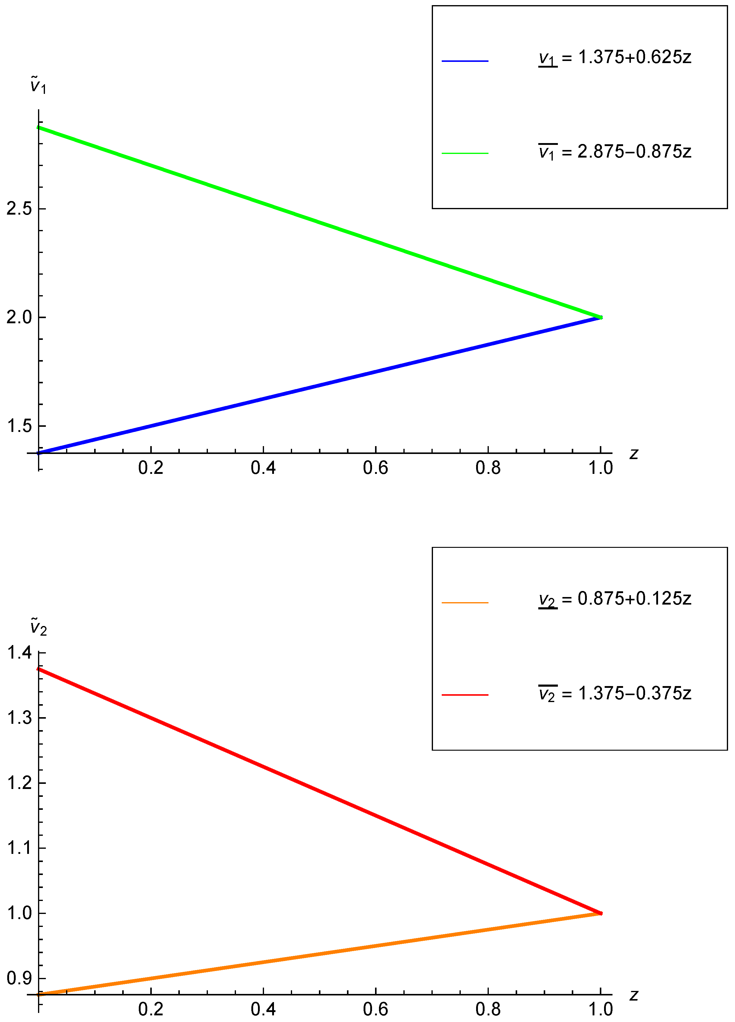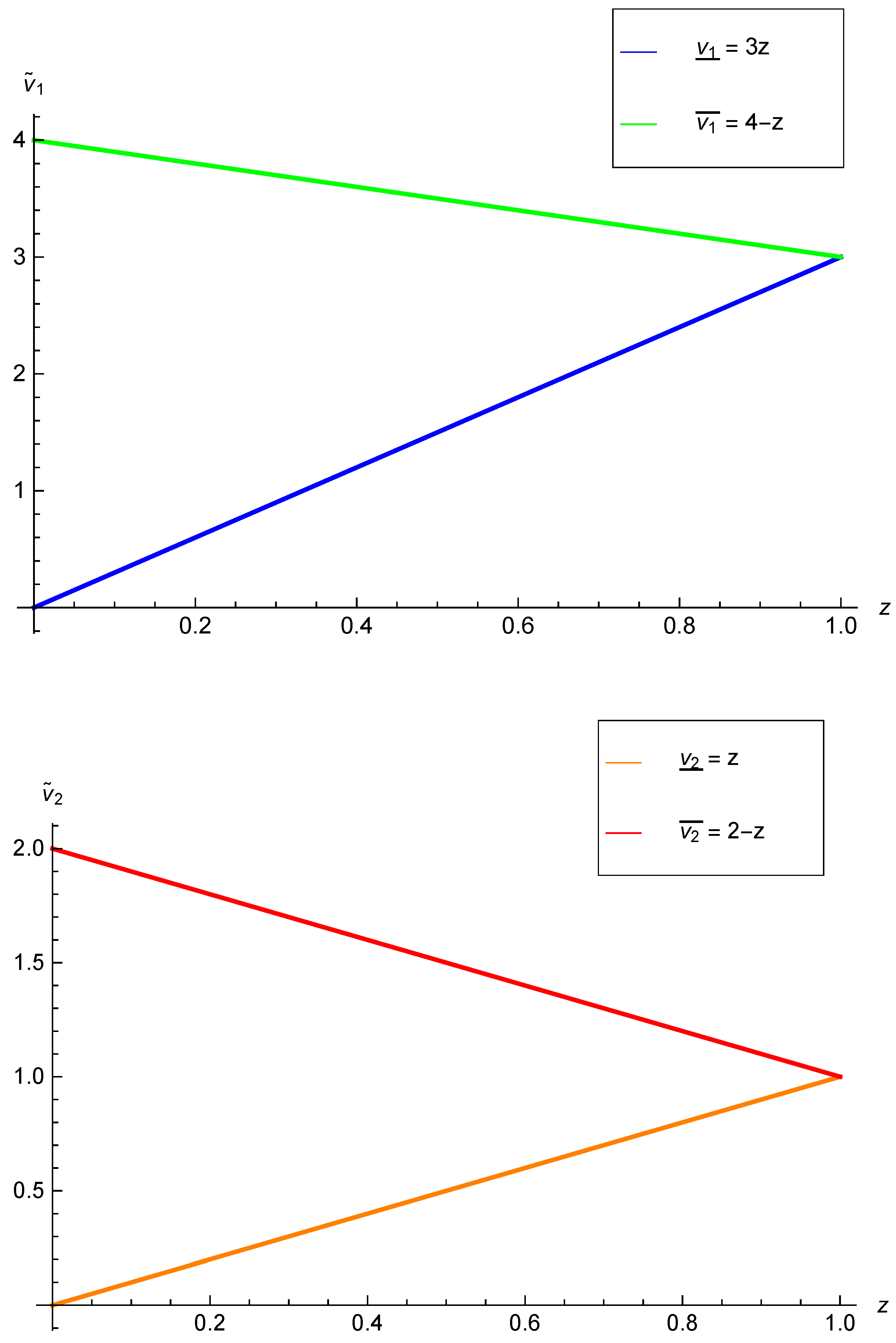In Section 4, several examples are solved by using the mentioned algorithms. Graphs of solutions are demonstrated to show that the obtained results are in the fuzzy form. Section 5 is the conclusion.

2. Preliminaries

In this paper, several definitions and details of fuzzy arithmetic are presented [4,5,6,9,10,36]. The methods of Friedman [9] and Ezzati [35] to solve the FSLEs are also considered. Ezzati’s method has some problems in proving the theorems that we modify and represent them.

Definition 1

([9,10]). Let $\tilde{p}=(\underline{p}(z),\overline{p}(z)),0\le z\le 1$ be the arbitrary fuzzy number then the following criteria should be satisfied:

(i) 

$\underline{p}(z)$ is a bounded monotonic increasing left continuous function;

(ii) 

$\overline{p}(z)$ is a bounded monotonic decreasing left continuous function;

(iii) 

$\underline{p}(z)\le \overline{p}(z),0\le z\le 1.$

The set of all fuzzy numbers is denoted by ${\mathbf{E}}^{\mathbf{1}}$. The crisp number k is called the singleton when $\overline{p}(z)=\underline{p}(z)=k,0\le z\le 1$.

Let $\tilde{p}=(\underline{p}(z),\overline{p}(z)),\tilde{q}=(\underline{q}(z),\overline{q}(z))$ be the arbitrary fuzzy functions and k be the scalar value. The operations between two fuzzy functions are defined as follows:

$$(\underline{p+q})(z)=\underline{p}(z)+\underline{q}(z),(\overline{p+q})(z)=\overline{p}(z)+\overline{q}(z),$$

(1)

$$(\underline{p-q})(z)=\underline{p}(z)-\overline{q}(z),(\overline{p-q})(z)=\overline{p}(z)-\underline{q}(z),$$

(2)

$$k\tilde{p}=\left\{\begin{array}{ll}{\displaystyle (k\underline{p}(z),k\overline{p}(z)),}& k\ge 0,\\ {\displaystyle (k\overline{p}(z),k\underline{p}(z)),}& k<0.\end{array}\right.$$

(3)

Also $\tilde{p}=\tilde{q}$ if and only if $\underline{p}(z)=\underline{q}(z)$ and $\overline{p}(z)=\overline{q}(z)$.

Remark 1.

The triangular fuzzy number $\tilde{p}=(c,\mu ,\rho )$ is defined as follows:

$$\tilde{p}=\left\{\begin{array}{ll}{\displaystyle \frac{x-c+\mu }{\mu },}& c-\mu \le x\le c,\\ {\displaystyle \frac{c+\rho -x}{\rho },}& c\le x\le c+\rho ,\\ {\displaystyle 0,}& o.w,\end{array}\right.$$

(4)

where $\mu ,\rho >0$. It is clear that $\underline{p}(z)=c-(1-z)\mu ,\overline{p}(z)=c+(1-z)\rho$, and $\overline{p}-\underline{p}=(\mu +\rho )(1-z)$. The set of all triangular fuzzy numbers is denoted by ${\mathbf{TE}}^{\mathbf{1}}$.

Definition 2

([9]). Let ${({\tilde{v}}_1,{\tilde{v}}_2,\dots ,{\tilde{v}}_j,\dots ,{\tilde{v}}_n)}^T,{\tilde{v}}_j=({\underline{v}}_j(z),{\overline{v}}_j(z)),1\le j\le n,0\le z\le 1$ be the fuzzy number vector which is called the solution of FSLEs if and only if:

$$\begin{array}{l}{\displaystyle \underline{\sum _{j=1}^n{a}_{ij}{v}_j}(z)=\sum _{j=1}^n\underline{a_{ij}{v}_j}(z)=\underline{b_i}(z),}\\ {\displaystyle \overline{\sum _{j=1}^n{a}_{ij}{v}_j}(z)=\sum _{j=1}^n\overline{a_{ij}{v}_j}(z)=\overline{b_i}(z),i=1,2,\cdots ,n.}\end{array}$$

(5)

Finally, the methods of Friedman et al. [9] and Ezzati [35] to solve the FSLEs is reminded.

2.1. Friedman’s Method

Friedman et al. [9] presented the FSLEs as:

$$Sv(z)=w(z),$$

(6)

where

$$\begin{array}{l}v(z)={\left({\underline{v}}_1(z),{\underline{v}}_2(z),\cdots ,{\underline{v}}_n(z),-{\overline{v}}_1(z),-{\overline{v}}_2(z),\cdots ,-{\overline{v}}_n(z)\right)}^T,\\ w(z)={\left({\underline{w}}_1(z),{\underline{w}}_2(z),\cdots ,{\underline{w}}_n(z),-{\overline{w}}_1(z),-{\overline{w}}_2(z),\cdots ,-{\overline{w}}_n(z)\right)}^T,\end{array}$$

(7)

and the elements of $S=(s_{ij}),1\le i,j\le 2n$ are obtained based on the following conditions:

$$\begin{array}{l}{a}_{ij}\ge 0\Rightarrow s_{ij}=s_{i+nj+n}=a_{ij},\\ a_{ij}<0\Rightarrow s_{ij+n}=s_{i+nj}=-a_{ij}.\end{array}$$

(8)

We note that for values $s_{ij}$ which are determined by neglecting the criterion in Equation (8) we have $s_{ij}=0$. The matrix S for $s_{ij}\ge 0,1\le i,j\le 2n$ can be formed as follows:

$$S=\left(\begin{array}{cc}B& C\\ C& B\end{array}\right),$$

(9)

where B constructs by the positive entries of A and C constructs by the absolute values of the negative entries of A and $A=B-C$.

For the nonsingular matrix S, we have $v(z)=S^{-1}w(z)$. However, there is a high likelihood that the obtained solution does not have the proper fuzzy number vector. Therefore, the solution of the FSLEs can be defined in the following form:

Definition 3

([9]). Let Equation (6) have the unique solution in the form $\tilde{v}(z)=\{({\underline{v}}_i(z),-{\overline{v}}_i(z)),1\le i\le n\}$. We define the fuzzy number vector $\tilde{P}=\{({\underline{p}}_i(z),{\overline{p}}_i(z)),1\le i\le n\}$ as:

$$\begin{array}{l}{\displaystyle {\underline{p}}_i(z)=min\{{\underline{v}}_i(z),{\overline{v}}_i(z),{\underline{v}}_i(1),{\overline{v}}_i(1)\},}\\ {\displaystyle {\overline{p}}_i(z)=max\{{\underline{v}}_i(z),{\overline{v}}_i(z),{\overline{v}}_i(1),{\underline{v}}_i(1)\},}\end{array}$$

(10)

which is called the fuzzy solution of Equation (6). If ${\underline{p}}_i(z)={\underline{v}}_i(z)$ and ${\overline{p}}_i(z)={\overline{v}}_i(z),1\le i\le n$ then $\tilde{P}$ is called a strong fuzzy solution. Otherwise, $\tilde{P}$ is called a weak fuzzy solution, which is not the solution of FSLE and is not always the fuzzy number vector.

Allahviranloo et al. [15] showed that a weak solution of a FSLE is not always a fuzzy number vector and it is the main fault of Friedman’s method.

2.2. Ezzati’s Method

Consider the following FSLEs:

$$\left\{\begin{array}{ll}{a}_{11}({\underline{v}}_1(z)+{\overline{v}}_1(z))+\dots +a_{1n}({\underline{v}}_n(z)+{\overline{v}}_n(z))& ={\underline{w}}_1(z)+{\overline{w}}_1(z),\\ a_{21}({\underline{v}}_1(z)+{\overline{v}}_1(z))+\dots +a_{2n}({\underline{v}}_n(z)+{\overline{v}}_n(z))& ={\underline{w}}_2(z)+{\overline{w}}_2(z),\\ ⋮& ⋮\\ a_{n1}({\underline{v}}_1(z)+{\overline{v}}_1(z))+\dots +a_{nn}({\underline{v}}_n(z)+{\overline{v}}_n(z))& ={\underline{w}}_n(z)+{\overline{w}}_n(z),\end{array}\right.$$

(11)

where the solution of system in Equation (11) is in the following form:

$$\mathbf{g}(\mathbf{z})=\left(\begin{array}{c}{g}_1(z)\\ g_2(z)\\ ⋮\\ g_n(z)\end{array}\right)=\underline{\mathbf{v}}(\mathbf{z})+\overline{\mathbf{v}}(\mathbf{z})=\left(\begin{array}{c}{\underline{v}}_1(z)+{\overline{v}}_1(z)\\ {\underline{v}}_2(z)+{\overline{v}}_2(z)\\ ⋮\\ {\underline{v}}_n(z)+{\overline{v}}_n(z)\end{array}\right).$$

(12)

Since $(B+C)\underline{v}(z)=\underline{w}(z)+Cg(z)$ and $(B+C)\overline{v}(z)=\overline{w}(z)+Cg(z)$, hence $\underline{v}(z)$ or $\overline{v}(z)$ can be determined by solving the following system:

$$\begin{array}{l}\underline{v}(z)={(B+C)}^{-1}(\underline{w}(z)+Cg(z)),\\ \overline{v}(z)={(B+C)}^{-1}(\overline{w}(z)+Cg(z)).\end{array}$$

(13)

Therefore, the solution of FSLEs in Equaiton (11) can be obtained by solving the system of Equation (13); that the vector of solution is unique. But it may still not be an appropriate fuzzy number vector.

Theorem 1

([35]). Let $\tilde{v}(z)={({\tilde{v}}_1(z),{\tilde{v}}_2(z),\dots ,{\tilde{v}}_n(z))}^T$ be the fuzzy solution of Equation (11) and the matrix ${\mathit{A}}^{-1}$ exists. Then the solution of system:

$$\mathit{A}(\overline{\mathit{v}}(z)+\underline{\mathit{v}}(z))=\overline{\mathit{w}}(z)+\underline{\mathit{w}}(z),$$

(14)

for $\overline{w}(z)+\underline{w}(z)={({\overline{w}}_1(z)+{\underline{w}}_1(z),{\overline{w}}_2(z)+{\underline{w}}_2(z),\dots ,{\overline{w}}_n(z)+{\underline{w}}_n(z))}^T$ is in the following form $\overline{v}(z)+\underline{v}(z)={({\overline{v}}_1(z)+{\underline{v}}_1(z),{\overline{v}}_2(z)+{\underline{v}}_2(z),\dots ,{\overline{v}}_n(z)+{\underline{v}}_n(z))}^T.$

Since the number of operations for solving $n\times n$ system are less than $2n\times 2n$ system, thus Ezzati’s method is better than Friedman’s method. In Theorem 4 of Ezzati’s method [35], the maximum number of multiplication operations (MNMOs) were obtained which has some failures. The modified form of this theorem is presented in the following form:

Theorem 2.

Let $F_n$ be the MNMOs of Friedman’s method for the solving system of Equation (6) with $v(z)={({\underline{v}}_1(z),{\underline{v}}_2(z),\dots ,{\underline{v}}_n(z),-{\overline{v}}_1(z),-{\overline{v}}_2(z),\dots ,-{\overline{v}}_n(z))}^T=S^{-1}w(z),$ and $E_n$ is the MNMOs of Ezzati’s method with $v(z)={({\underline{v}}_1(z),{\underline{v}}_2(z),\dots {\underline{v}}_n(z),{\overline{v}}_1(z),{\overline{v}}_2(z),\dots ,{\overline{v}}_n(z))}^T,$ then $F_n\ge E_n$ and $F_n-E_n=2n^2$.

Proof. 

Suppose $h_n(A)$ is the MNMOs of computing the matrix $A^{-1}$. Now, we can write:

$${\mathbf{S}}^{-\mathbf{1}}=\left(\begin{array}{cc}D& E\\ E& D\end{array}\right),$$

(15)

where ${\displaystyle D=\frac{1}{2}[{(B+C)}^{-1}+{(B-C)}^{-1}],}$ and ${\displaystyle E=\frac{1}{2}[{(B+C)}^{-1}-{(B-C)}^{-1}]}$. Therefore, in order to determine $S^{-1}$, computing matrices ${(B+C)}^{-1}$ and ${(B-C)}^{-1}$ are required. It is clear that $h_n(S)=h_n(B+C)+h_n(B-C)=2h_n(A).$ Since $\tilde{v}(z)\in E^1$; $\underline{v}(z)$ and $\overline{v}(z)$, in the simplest case are lines hence $F_n=2h_n(A)+8n^2$. For computing $\underline{v}(z)+\overline{v}(z)={({\underline{v}}_1(z)+{\overline{v}}_1(z),{\underline{v}}_2(z)+{\overline{v}}_2(z),\dots ,{\underline{v}}_n(z)+{\overline{v}}_n(z))}^T$ from Equation (11) and $\underline{v}(z)={({\underline{v}}_1(z),{\underline{v}}_2(z),\dots {\underline{v}}_n(z))}^T$ from Equation (13) and according to Ezzati’s method, the MNMOs are $h_n(A)+2n^2$ and $h_n(B+C)+4n^2$, respectively. Since $h_n(B+C)=h_n(A)$ thus $E_n=2h_n(A)+6n^2,$ and finally $F_n-E_n=2n^2.$ ☐

Definition 4

([35]). Assume $\tilde{v}(z)=\{({\underline{v}}_i(z),{\overline{v}}_i(z)),1\le i\le n\}$ is the unique solution of Equations (11) and (13). The fuzzy number vector $\tilde{P}=\{({\underline{p}}_i(z),{\overline{p}}_i(z)),1\le i\le n\}$ is defined by:

$$\begin{array}{l}{\underline{p}}_i(z)=min\{{\underline{v}}_i(z),{\overline{v}}_i(z),{\underline{v}}_i(1)\},\\ {\overline{p}}_i(z)=max\{{\underline{v}}_i(z),{\overline{v}}_i(z),{\overline{v}}_i(1)\},\end{array}$$

(16)

which is called a fuzzy vector solution of Equations (11) and (13).

If ${\underline{p}}_i(z)={\underline{v}}_i(z)$ and ${\overline{p}}_i(z)={\overline{v}}_i(z),1\le i\le n,$ then $\tilde{P}$ is called a strong fuzzy solution. Otherwise, $\tilde{P}$ is called a weak fuzzy solution which is not the fuzzy linear system’s solution and is not always a fuzzy number vector.

Remark 2.

We know that Friedman et al. [9] and Ezzati [35] found two kinds of solutions, which are called the weak and strong solutions. The weak solution is not the system’s solution and it is not always the fuzzy number vector [15]. Hence, finding the weak fuzzy solution is not an interesting problem. Furthermore, in these methods the kind of solutions (strong or weak) can be determined only in the end of solving process and is one of the important faults of these methods.

In the next section, a novel method for solving $n\times n$ FSLEs is presented. Based on this method we can decrease the computing error because without carrying out a further computation, we can determine that the fuzzy linear system has no fuzzy number vector solution.

3. Proposed Method

In this section, a novel and applicable method to solve the FSLEs is presented. Several theorems and lemmas are illustrated to improve Ezzati’s method [35]. By using these theorems we show the number of operations of our method are less than the methods of Ezzati [35] and Friedman [9].

Theorem 3.

Suppose that the inverse matrix ofB + Cexists and $\tilde{v}(z)={({\tilde{v}}_1(z),{\tilde{v}}_2(z),\dots ,{\tilde{v}}_n(z))}^T$ is a fuzzy solution of Equation (11). Then $\overline{v}(z)-\underline{v}(z)={\left({\overline{v}}_1(z)-{\underline{v}}_1(z),{\overline{v}}_2(z)-{\underline{v}}_2(z),\dots ,{\overline{v}}_n(z)-{\underline{v}}_n(z)\right)}^T$ is the solution of the following system:

$$(\mathit{B}+\mathit{C})(\overline{\mathit{v}}(z)-\underline{\mathit{v}}(z))=\overline{\mathit{w}}(z)-\underline{\mathit{w}}(z),$$

(17)

where $\overline{w}(z)-\underline{w}(z)={({\overline{w}}_1(z)-{\underline{w}}_1(z),{\overline{w}}_2(z)-{\underline{w}}_2(z),\dots ,{\overline{w}}_n(z)-{\underline{w}}_n(z))}^T.$

Proof. 

Let ${\tilde{v}}_j(z)=({\underline{v}}_j(z),{\overline{v}}_j(z)),1\le j\le n$ be the parametric form of ${\tilde{v}}_j$. For positive values $a_{ij}^{\prime }$ and $a_{ij}^{″}$ we have $a_{ij}=a_{ij}^{\prime }-a_{ij}^{″}$ and $a_{ij}^{\prime }{a}_{ij}^{″}=0$ where $a_{ij},a_{ij}^{\prime }$ and $a_{ij}^{″}$ are the coefficients of matrices A, B, and C respectively. By presenting Equation (11) to the parametric form, for $i=1,2,\dots ,n$ we get:

$$(a_{i1}^{\prime }-a_{i1}^{″})({\underline{v}}_1(z),{\overline{v}}_1(z))+\dots +(a_{in}^{\prime }-a_{in}^{″})({\underline{v}}_n(z),{\overline{v}}_n(z))=({\underline{w}}_i(z),{\overline{w}}_i(z)).$$

(18)

Hence,

$$\begin{array}{c}{a}_{i1}^{\prime }{\underline{v}}_1(z)-a_{i1}^{″}{\overline{v}}_1(z)+a_{i2}^{\prime }{\underline{v}}_2(z)-a_{i2}^{″}{\overline{v}}_2(z)+\dots +a_{in}^{\prime }{\underline{v}}_n(z)-a_{in}^{″}{\overline{v}}_n(z)={\underline{w}}_i(z),\end{array}$$

(19)

and

$$\begin{array}{c}{a}_{i1}^{\prime }{\overline{v}}_1(z)-a_{i1}^{″}{\underline{v}}_1(z)+a_{i2}^{\prime }{\overline{v}}_2(z)-a_{i2}^{″}{\underline{v}}_2(z)+\dots +a_{in}^{\prime }{\overline{v}}_n(z)-a_{in}^{″}{\underline{v}}_n(z)={\overline{w}}_i(z).\end{array}$$

(20)

Now, using Equation (19) from Equation (20) we can write:

$$(a_{i1}^{\prime }+a_{i2}^{″})({\overline{v}}_1(z)-{\underline{v}}_1(z))+(a_{i2}^{\prime }+a_{i2}^{″})({\overline{v}}_2(z)-{\underline{v}}_2(z))+\dots +(a_{in}^{\prime }+a_{in}^{″})({\overline{v}}_n(z)-{\underline{v}}_n(z))={\overline{w}}_i(z)-{\underline{w}}_i(z).$$

(21)

Therefore, $d(z)=\overline{v}(z)-\underline{v}(z)={({\overline{v}}_1(z)-{\underline{v}}_1(z),{\overline{v}}_2(z)-{\underline{v}}_2(z),\dots ,{\overline{v}}_n(z)-{\underline{v}}_n(z))}^T$ is the solution of $(B+C)(\overline{v}(z)-\underline{v}(z))=\overline{w}(z)-\underline{w}(z)$. ☐

Theorem 4.

Suppose the inverse matrix ofB + Cexists. Equation (11) does not have a fuzzy number vector solution, if the vector solution of the following system is not non-negative, i.e., at least one of the entries are negative:

$$(\mathit{B}+\mathit{C})(\overline{\mathit{v}}(z)-\underline{\mathit{v}}(z))=\overline{\mathit{w}}(z)-\underline{\mathit{w}}(z).$$

(22)

Proof. 

We know that, the vector solution of Equation (22) is $\overline{v}(z)-\underline{v}(z)$. Now, suppose that $\overline{v}(z)-\underline{v}(z)$ is not non-negative. So, according to Definition 1, the fuzzy number vector solution does not exist. It is clear that the matrix ${(B+C)}^{-1}$ is the non-positive matrix, i.e., at least one of the entries is positive because $(B+C)$ is the positive matrix. ☐

Triangular fuzzy numbers are simple and popular fuzzy numbers. Triangular fuzzy numbers also have a special property $\overline{w}(z)-\underline{w}(z)=({\rho }^{\prime }+{\rho }^{″})(1-z).$ Hence when the right-hand side vector $\tilde{w}(z)$ is triangular, the parametric linear system of Equation (22) can be transformed into the crisp linear system.

Lemma 1.

Suppose that the inverse matrix of $(B+C)$ exists, and $\tilde{w}(z)\in T{E}^1$. Equation (11) does not have a fuzzy number vector solution, if the vector solution of the following system is not non-negative, i.e., at least one of the entries is negative:

$$(B+C)({\mu }^{\prime }+{\mu }^{″})=({\rho }^{\prime }+{\rho }^{″}),$$

(23)

where $({\mu }^{\prime }+{\mu }^{″})(1-z)=\overline{v}(z)-\underline{v}(z),({\rho }^{\prime }+{\rho }^{″})(1-z)=\overline{w}(z)-\underline{w}(z).$

Now, a new method to solve the FSLEs is presented. Assume that the inverse matrix of A in Equation (11) exists. For solving Equation (11), the following system:

$$(\mathbf{B}+\mathbf{C})(\overline{\mathbf{v}}(z)-\underline{\mathbf{v}}(z))=\overline{\mathbf{w}}(z)-\underline{\mathbf{w}}(z),$$

(24)

should be solved where the matrices B and C were defined in Section 2.2. Let the solution of this system be in the following form:

$$\mathbf{d}(\mathbf{z})=\left(\begin{array}{c}{d}_1(z)\\ d_2(z)\\ ⋮\\ d_n(z)\end{array}\right)=\overline{\mathbf{v}}(\mathbf{z})-\underline{\mathbf{v}}(\mathbf{z})=\left(\begin{array}{c}{\overline{v}}_1(z)-{\underline{v}}_1(z)\\ {\overline{v}}_2(z)-{\underline{v}}_2(z)\\ ⋮\\ {\overline{v}}_n(z)-{\underline{v}}_n(z)\end{array}\right).$$

(25)

If $d=\overline{v}-\underline{v}$ is not non-negative, then we do not have the fuzzy number vector solution. Otherwise, in order to show the existence of fuzzy number vector solution for Equation (11), we continue our idea. At first, we should solve the following system:

$$\mathbf{A}(\overline{\mathbf{v}}(z)+\underline{\mathbf{v}}(z))=\overline{\mathbf{w}}(z)+\underline{\mathbf{w}}(z).$$

(26)

According to Theorem 1, we know that this system has the solution in the following form:

$$\mathbf{g}(\mathbf{z})=\left(\begin{array}{c}{g}_1(z)\\ g_2(z)\\ ⋮\\ g_n(z)\end{array}\right)=\overline{\mathbf{v}}(\mathbf{z})+\underline{\mathbf{v}}(\mathbf{z})=\left(\begin{array}{c}{\overline{v}}_1(z)+{\underline{v}}_1(z)\\ {\overline{v}}_2(z)+{\underline{v}}_2(z)\\ ⋮\\ {\overline{v}}_n(z)+{\underline{v}}_n(z)\end{array}\right).$$

(27)

Finally, by solving systems of Equations (24) and (26) and finding $\mathbf{d}(\mathbf{z})$ and $\mathbf{g}(\mathbf{z})$ we have:

$$\left\{\begin{array}{c}\underline{v}(z)=\frac{\mathbf{g}(\mathbf{z})-\mathbf{d}(\mathbf{z})}{2},\\ \overline{v}(z)=\frac{\mathbf{g}(\mathbf{z})+\mathbf{d}(\mathbf{z})}{2}.\end{array}\right.$$

(28)

If the conditions of Definition 1 are satisfied, then the solution of FSLEs for Equation (11) can be obtained by solving the crisp linear system of Equations (24) and (26) that the solution vector is the fuzzy number vector and unique. Otherwise, if at least one of the conditions is not true, the fuzzy linear system of Equation (11) does not have a fuzzy number vector solution.

Remark 3.

If $\tilde{w}\in T{E}^1$, then according to Lemma 1 the system of Equation (24) have the vector solution as $d^{\prime }={\mu }^{\prime }+{\mu }^{″}$ where $d(z)=d^{\prime }(1-z)$. So, Equation (28) can be written in the following form:

$$\left\{\begin{array}{c}\underline{v}(z)=\frac{\mathbf{g}(\mathbf{z})-{\mathbf{d}}^{\prime }(\mathbf{1}-\mathbf{z})}{2},\\ \overline{v}(z)=\frac{\mathbf{g}(\mathbf{z})+{\mathbf{d}}^{\prime }(\mathbf{1}-\mathbf{z})}{2}.\end{array}\right.$$

(29)

Theorem 5.

Assume that n is any integer, $n\ge 2$, and denote by $E_n$ and $D_n$ the MNMOs that are required to calculate $v(z)={({\underline{v}}_1(z),{\underline{v}}_2(z),\dots {\underline{v}}_n(z),{\overline{v}}_1(z),{\overline{v}}_2(z),\dots ,{\overline{v}}_n(z))}^T,$ in Ezzati’s method [35] and presented method then:

$$\left\{\begin{array}{ll}{E}_n-D_n=2n^2,& \overline{v}(z)-\underline{v}(z)\ge 0,\\ E_n-D_n=h_n(A)+4n^2,& o.w.,\end{array}\right.$$

(30)

where $h_n(A)$ shows the MNMOs that are required to calculate $A^{-1}$.

Proof. 

According to Theorem 2, we have $E_n=2h_n(A)+6n^2.$ Assume $d(z)=\overline{v}(z)-\underline{v}(z)$ is the non-negative matrix then in order to know that the fuzzy linear system of Equation (11) has the fuzzy number vector solution, we need to solve the system of Equation (26). So, for computing $\overline{v}(z)-\underline{v}(z)={({\overline{v}}_1(z)-{\underline{v}}_1(z),{\overline{v}}_2(z)-{\underline{v}}_2(z),\dots ,{\overline{v}}_n(z)-{\underline{v}}_n(z))}^T,$ and $\overline{v}(z)+\underline{v}(z)={({\overline{v}}_1(z)+{\underline{v}}_1(z),{\overline{v}}_2(z)+{\underline{v}}_2(z),\dots ,{\overline{v}}_n(z)+{\underline{v}}_n(z))}^T,$ from Equations (24) and (26), the maximum number of multiplication operations are $h_n(B+C)+2n^2$ and $h_n(A)+2n^2$, respectively. Clearly $h_n(B+C)=h_n(A)$. Hence $D_n=2h_n(A)+4n^2$ and $E_n-D_n=2n^2.$

Otherwise, assume that $d(z)=\overline{v}(z)-\underline{v}(z)$ is not the non-negative matrix. According to Theorem 4 we do not have the fuzzy number vector solution for solving the FSLEs of Equation (11). If we do not have the fuzzy number vector solution, computing $\overline{v}(z)+\underline{v}(z)$ from the system of Equation (26) will be unnecessary. Thus, we need to compute $d(z)=\overline{v}(z)-\underline{v}(z)$. Therefore, in this case, the maximum number of multiplication operations are $h_n(B+c)+2n^2$ or $h_n(A)+2n^2$. Finally, we have $E_n\ge D_n,E_n-D_n=h_n(A)+4n^2.$ ☐

Lemma 2.

Let $\tilde{w}(z)$ be the triangular fuzzy number vector from Equation (11). Then $\tilde{v}(z)$ is the triangular fuzzy number vector solution from Equation (11).

Lemma 3.

Suppose that in Theorem 5, $\tilde{w}(z)$ is the triangular fuzzy number vector from Equation (11), then $E_n\ge D_n$ and

$$\left\{\begin{array}{ll}{E}_n-D_n=3n^2-n,& \overline{v}(z)-\underline{v}(z)\ge 0,\\ E_n-D_n=h_n(A)+5n^2,& o.w.\end{array}\right.$$

(31)

Proof. 

If $\tilde{w}(z)$ is the triangular fuzzy number vector from Equation (11) i.e., since $\tilde{w}(z)\in T{E}^1;\underline{w}(z)$ and $\overline{w}(z)$ in the simplest case is the line. So clearly, according to Theorem 2, we have $E_n=2h_n(A)+6n^2,$ and according to Remark 1, we get $\overline{v}(z)=c+(1-z){\mu }^{\prime }$ and $\underline{v}(z)=c-(1-z){\mu }^{″}.$ So, $\overline{v}(z)-\underline{v}(z)=({\mu }^{\prime }+{\mu }^{″})(1-z)$ and $\overline{w}(z)-\underline{w}(z)=({\rho }^{\prime }+{\rho }^{″})(1-z),$ and from the system of Equation (24), we have:

$$(B+C)({\mu }^{\prime }+{\mu }^{″})(1-z)=({\rho }^{\prime }+{\rho }^{″})(1-z).$$

(32)

If $r\ne 1$, the following relation can be obtained as:

$$(B+C)({\mu }^{\prime }+{\mu }^{″})={\rho }^{\prime }+{\rho }^{″},$$

(33)

where it is the crisp linear system. It is clear that for $r=1$, the FSLE can be replaced by crisp linear system.

Now, we assume that $d^{\prime }=({\mu }^{\prime }+{\mu }^{″})$ is non-negative. Then for understanding that whether the FSLEs of Equation (11) has the fuzzy number vector solution, we need to solve the system of Equation (26). So, for computing $({\mu }^{\prime }+{\mu }^{″})=({\mu }_1^{\prime }+{\mu }_1^{″},{\mu }_2^{\prime }+{\mu }_2^{″},\dots ,{\mu }_n^{\prime }+{\mu }_n^{″})$ from Equation (33) and $\overline{v}(z)+\underline{v}(z)={({\overline{v}}_1(z)+{\underline{v}}_1(z),{\overline{v}}_2(z)+{\underline{v}}_2(z),\dots ,{\overline{v}}_n(z)+{\underline{v}}_n(z))}^T$ from Equation (26) and $d(z)=(1-z)d^{\prime }$ for the final solution in Equation (29) the maximum number of multiplication operations are $h_n(B+C)+n^2$, $h_n(A)+2n^2$ and n respectively. Clearly $h_n(B+C)=h_n(A)$. So $D_n=2h_n(A)+3n^2+n,$ and

$$E_n\ge D_n,E_n-D_n=3n^2-n.$$

(34)

Otherwise, assume that $d^{\prime }=({\mu }^{\prime }+{\mu }^{″})$ is not non-negative. Then, according to Lemma 1 we do not have a fuzzy number vector solution for solving the fuzzy linear system of Equation (11). We know that if we do not have a fuzzy number vector solution, there is no necessity for computing $\underline{v}(z)+\overline{v}(z)$ from Equation (26). Thus, we need to compute $d^{\prime }=({\mu }^{\prime }+{\mu }^{″})$. Therefore, in this case the maximum number of multiplication operations are $h_n(B+C)+n^{2}or{h}_n(A)+n^2.$ Then, we have $E_n\ge D_n,E_n-D_n=h_n(A)+5n^2.$ ☐

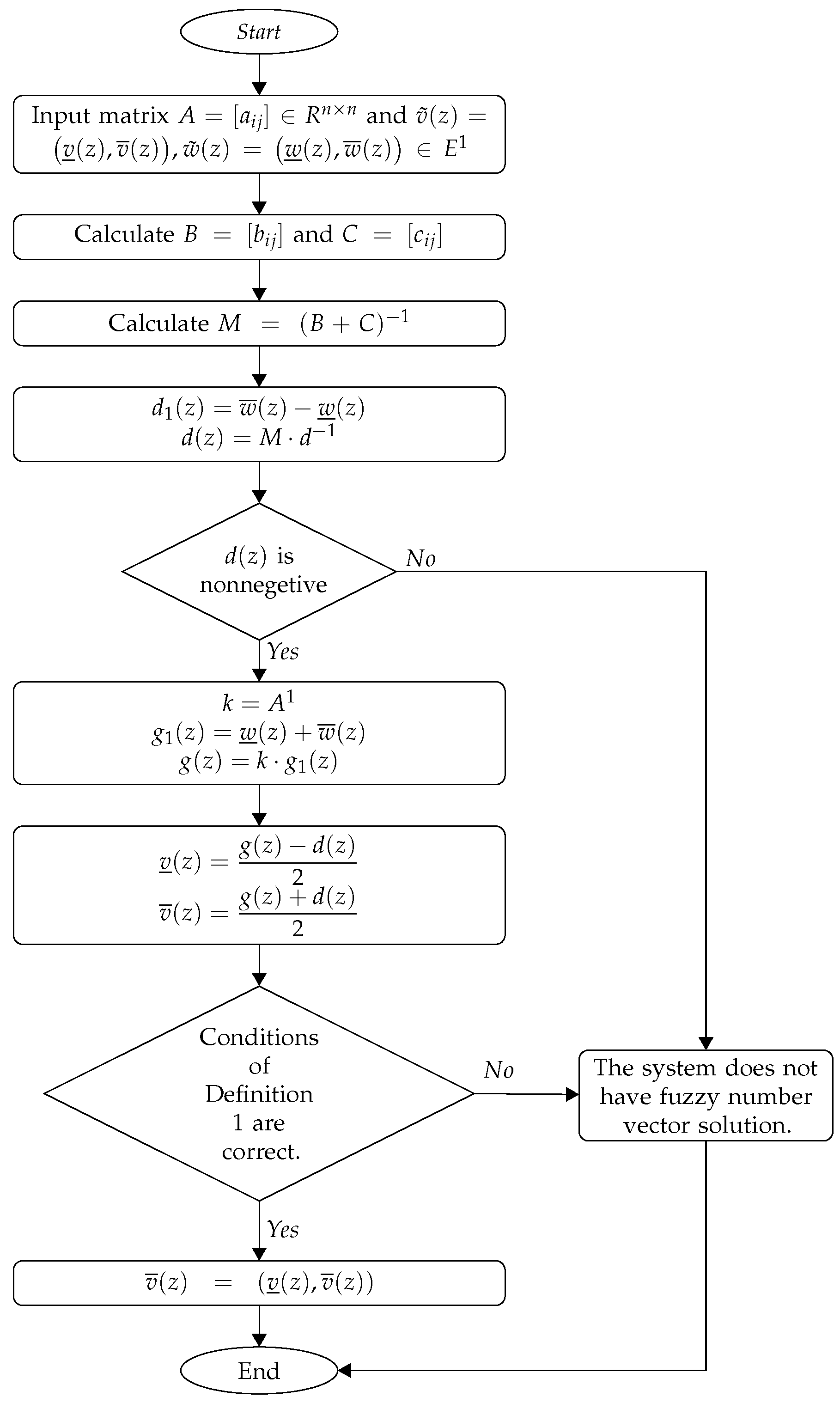
Method’s Algorithms

In Figure 1 and Figure 2, the flowcharts of mentioned algorithms are presented.

Algorithm 1: Let A be the nonsingular matrix.

Step 1: Input matrix $A=\left[a_{ij}\right]\in R^{n\times n}$ and $\tilde{v}(z)=(\underline{v}(z),\overline{v}(z)),\tilde{w}(z)=(\underline{w}(z),\overline{w}(z))\in E^1$. Step 2: Calculate $B=\left[b_{ij}\right]$ and $C=\left[c_{ij}\right]$ as $$\left\{\begin{array}{ll}If{a}_{ij}>0\Rightarrow b_{ij}=a_{ij};& else{b}_{ij}=0,\\ If{a}_{ij}<0\Rightarrow c_{ij}=-a_{ij};& else{c}_{ij}=0.\end{array}\right.$$ Step 3: Calculate $M={(B+C)}^{-1}$. Step 4: Calculate $d_1(z)=\overline{w}(z)-\underline{w}(z)$ and $d(z)=M.d_1(z)$. If $d(z)$ is not nonnegative, go to Step 8. Step 5: Calculate $k=A^{-1},g_1(z)=\overline{w}(z)+\underline{w}(z)$ and $g(z)=k.g_1(z)$. Step 6: Calculate $\underline{v}(z)=\frac{g(z)-d(z)}{2}$ and $\overline{v}(z)=\frac{g(z)+d(z)}{2}$. Step 7: If conditions of Definition 1 are true then $\tilde{v}(z)=(\underline{v}(z),\overline{v}(z))$ and go to Step 9. Else go to Step 8. Step 8: Show the message "The system does not have fuzzy number vector solution". Step 9: End.

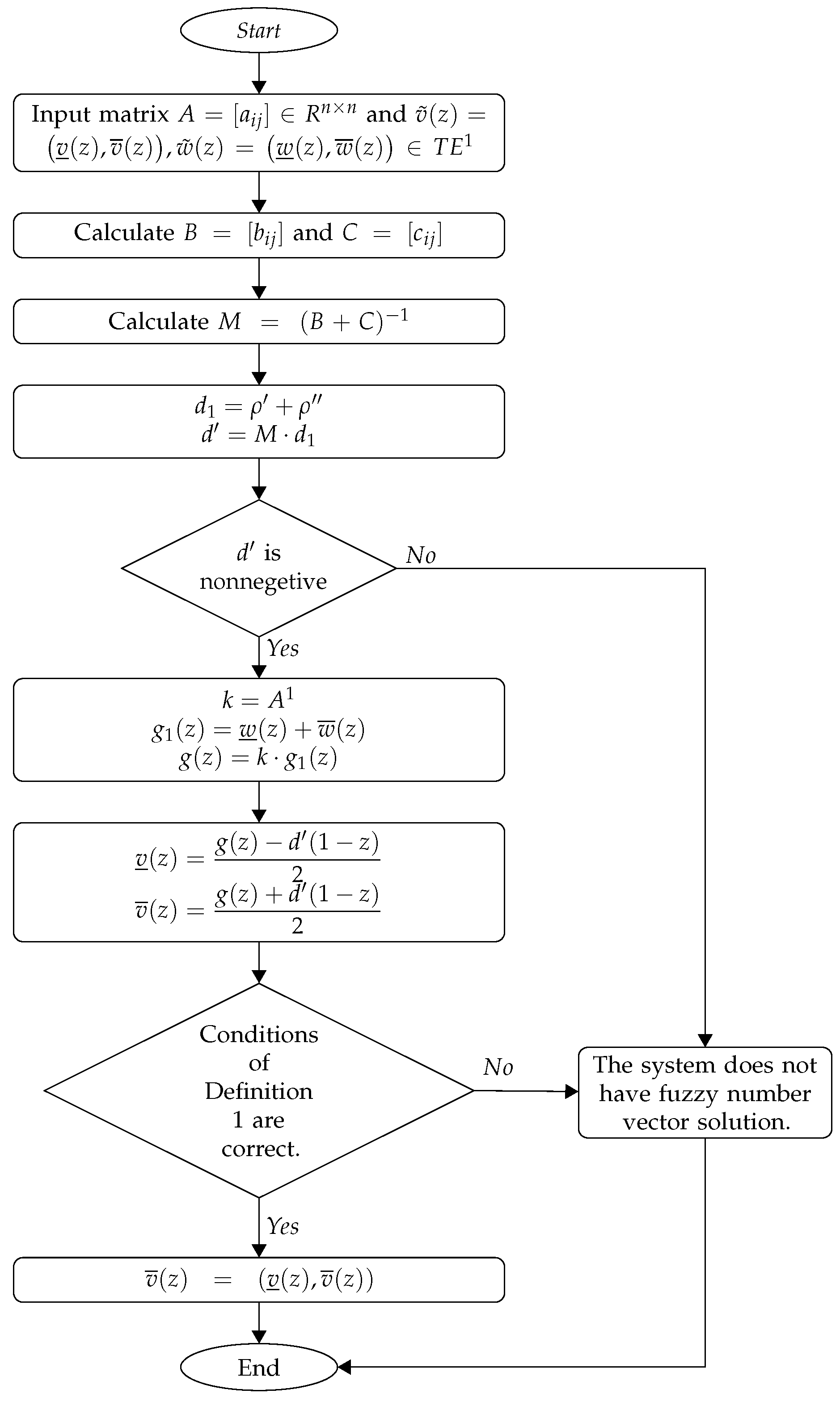
Algorithm 2: The following algorithm is presented to triangular fuzzy linear system.

Step 1: Input matrix $A=\left[a_{ij}\right]\in R^{n\times n}$ and $\tilde{v}(z)=(\underline{v}(z),\overline{v}(z)),\tilde{w}(z)=(\underline{w}(z),\overline{w}(z))\in T{E}^1$. Step 2: Calculate $B=\left[b_{ij}\right]$ and $C=\left[c_{ij}\right]$ as $$\left\{\begin{array}{ll}If{a}_{ij}>0\Rightarrow b_{ij}=a_{ij};& else{b}_{ij}=0,\\ If{a}_{ij}<0\Rightarrow c_{ij}=-a_{ij};& else{c}_{ij}=0.\end{array}\right.$$ Step 3: Calculate $M={(B+C)}^{-1}$. Step 4: Calculate $d_1={\rho }^{\prime }+{\rho }^{″}$ and $d^{\prime }=M.d_1$. If $d^{\prime }$ is not nonnegative, go to Step 8. Step 5: Calculate $k=A^{-1},g_1(z)=\overline{w}(z)+\underline{w}(z)$ and $g(z)=k.g_1(z)$. Step 6: Calculate $\underline{v}(z)=\frac{g(z)-d^{\prime }(1-z)}{2};$ and $\overline{v}(z)=\frac{g(z)+d^{\prime }(1-z)}{2}$. Step 7: If conditions of Definition 1 are true then $\tilde{v}(z)=(\underline{v}(z),\overline{v}(z))$ and go to Step 9. Else go to Step 8. Step 8: Show the message "The system does not have fuzzy number vector solution". Step 9: End.

4. Numerical Illustrations

In this section, some examples of the FSLEs are presented [9]. Furthermore, several graphs are demonstrated to show that the obtained solutions are fuzzy vector solutions.

Example 1

([9]). Consider the following $2\times 2$ FSLEs:

$$\left\{\begin{array}{l}{\tilde{v}}_1-{\tilde{v}}_2=(z,2-z),\\ {\tilde{v}}_1+3{\tilde{v}}_2=(4+z,7-2z),\end{array}\right.$$

(35)

where $\tilde{w}$ is a triangular vector of fuzzy numbers hence Algorithm 2 is applied. By using this algorithm we have:

• Step 1.Input matrix:

  $$A=\left(\begin{array}{cc}1& -1\\ 1& 3\end{array}\right),$$

  (36)

  $$\tilde{v}(z)=(\underline{v}(z),\overline{v}(z))\in T{E}^1,\tilde{w}(z)=(\underline{w}(z),\overline{w}(z))=\left(\begin{array}{c}(z,2-z)\\ (4+z,7-2z)\end{array}\right).$$

  (37)
• Step 2.Calculate:

  $$B=\left[b_{ij}\right]=\left(\begin{array}{cc}1& 0\\ 1& 3\end{array}\right),C=\left[c_{ij}\right]=\left(\begin{array}{cc}0& 1\\ \\ 0& 0\end{array}\right).$$

  (38)
• Step 3.Compute:

  $$M={(B+C)}^{-1}=\left(\begin{array}{cc}{\displaystyle \frac{3}{2}}& {\displaystyle -\frac{1}{2}}\\ \\ {\displaystyle -\frac{1}{2}}& {\displaystyle \frac{1}{2}}\end{array}\right).$$

  (39)
• Step 4.Calculate:

  $$d_1={\rho }^{\prime }+{\rho }^{″}=\left(\begin{array}{c}{\rho }_1^{\prime }+{\rho }_1^{″}\\ {\rho }_2^{\prime }+{\rho }_2^{″}\end{array}\right)=\left(\begin{array}{c}2\\ 3\end{array}\right),d^{\prime }=M.d_1=\left(\begin{array}{c}{\displaystyle \frac{3}{2}}\\ {\displaystyle \frac{1}{2}}\end{array}\right).$$

  (40)

  It is clear that $d^{\prime }={\mu }^{\prime }+{\mu }^{″}$ is the non-negative matrix, therefore go to the Step 5.
• Step 5.Calculate:

  $$k=A^{-1}=\left(\begin{array}{cc}{\displaystyle \frac{3}{4}}& {\displaystyle \frac{1}{4}}\\ {\displaystyle -\frac{1}{4}}& {\displaystyle \frac{1}{4}}\end{array}\right),g_1(z)=\overline{w}(z)+\underline{w}(z)=\left(\begin{array}{c}2\\ 11-z\end{array}\right),$$

  (41)

  $$g(z)=k.g_1(z)=\left(\begin{array}{c}{\displaystyle \frac{17-z}{4}}\\ {\displaystyle \frac{9-z}{4}}\end{array}\right).$$

  (42)
• Step 6.Compute:

  $$\underline{v}(z)=\frac{g(z)-d(z)}{2}=\left(\begin{array}{c}{\underline{v}}_1\\ {\underline{v}}_2\end{array}\right)=\left(\begin{array}{c}1.375+0.625z\\ 0.875+0.125z\end{array}\right),$$

  (43)

  $$\overline{v}(z)=\frac{g(z)+d(z)}{2}=\left(\begin{array}{c}{\overline{v}}_1\\ {\overline{v}}_2\end{array}\right)=\left(\begin{array}{c}2.875-0.875z\\ 1.375-0.375z\end{array}\right).$$

  (44)

Since the conditions of Definition 1 are satisfied, the FSLEs has the fuzzy number vector solution. Now, we can show that the MNMOs of the presented method are less than the MNMOs of Friedman and Ezzati’s methods. Suppose $h_n(A)$ is the MNMOs of $A^{-1}$ and $F_n$, $E_n$ and $D_n$ are the MNMOs obtained from Friedman’s method, Ezzati’s method and the proposed method, respectively. So for $n=2$ we have:

$$\begin{array}{l}{F}_n=2h_n(A)+8n^2=2h_n(A)+32,\\ E_n=2h_n(A)+6n^2=2h_n(A)+24,\\ D_n=2h_n(A)+3n^2+n=2h_n(A)+14,\end{array}$$

and it is obvious that $D_n<E_n<F_n$. In Figure 3, the obtained solutions are presented for $z\in [0,1]$. Based on this figure we can clearly see that the obtained results are the fuzzy number vector solutions.

Example 2

([9]). Consider the $3\times 3$ FSLEs:

$$\left\{\begin{array}{l}{\tilde{v}}_1+{\tilde{v}}_2-{\tilde{v}}_3=(z,2-z),\\ {\tilde{v}}_1-2{\tilde{v}}_2+{\tilde{v}}_3=(2+z,3),\\ 2{\tilde{v}}_1+{\tilde{v}}_2+3{\tilde{v}}_3=(-2,-1-z),\end{array}\right.$$

(45)

where $\tilde{Y}$ is a triangular fuzzy number vector. By using Algorithm 2 we have:

• Step 1.Input matrix:

  $$A=\left(\begin{array}{ccc}1& 1& -1\\ & \\ 1& -2& 1\\ & \\ 2& 1& 3\end{array}\right),\tilde{w}(z)=(\underline{w}(z),\overline{w}(z))=\left(\begin{array}{c}(z,2-z)\\ (2+z,3)\\ (-2,-1-z)\end{array}\right).$$

  (46)
• Step 2.Compute:

  $$B=\left[b_{ij}\right]=\left(\begin{array}{ccc}1& 1& 0\\ & \\ 1& 0& 1\\ & \\ 2& 1& 3\end{array}\right),C=\left[c_{ij}\right]=\left(\begin{array}{ccc}0& 0& 1\\ & \\ 0& 2& 0\\ & \\ 0& 0& 0\end{array}\right).$$

  (47)
• Step 3.Calculate:

  $$M={(B+C)}^{-1}=\left(\begin{array}{ccc}5& -1& -3\\ -2& 1& 1\\ -1& 0& 1\end{array}\right).$$

  (48)
• Step 4.Compute:

  $$d_1={\rho }^{\prime }+{\rho }^{″}=\left(\begin{array}{c}{\rho }_1^{\prime }+{\rho }_1^{″}\\ {\rho }_2^{\prime }+{\rho }_2^{″}\end{array}\right)=\left(\begin{array}{c}2\\ 1\\ 1\end{array}\right),d^{\prime }=M.d_1=\left(\begin{array}{c}6\\ -2\\ -1\end{array}\right).$$

  (49)

Since $d^{\prime }={\mu }^{\prime }+{\mu }^{″}$ is not non-negative, therefore the system does not have a fuzzy number vector solution. In order to show the MNMOs of mentioned methods for $n=3$ we get:

$$\begin{array}{l}{F}_n=2h_n(A)+8n^2=2h_n(A)+72,\\ E_n=2h_n(A)+6n^2=2h_n(A)+54,\\ D_n=2h_n(A)+n^2=2h_n(A)+9.\end{array}$$

In this case, we have $D_n<E_n<F_n$ and it shows that MNMOs of the presented method is less than two other methods.

Example 3.

Consider the following $2\times 2$ FSLEs:

$$\left\{\begin{array}{c}{\tilde{v}}_1+{\tilde{v}}_2=(4z,6-2z),\\ {\tilde{v}}_1+2{\tilde{v}}_2=(5z,8-3z).\end{array}\right.$$

(50)

In this example, by applying Algorithm 1 we have:

• Step 1.Input matrix:

  $$A=\left(\begin{array}{cc}1& 1\\ \\ 1& 2\end{array}\right),\tilde{w}(z)=(\underline{w}(z),\overline{w}(z))=\left(\begin{array}{c}(4z,6-2z)\\ (5z,8-3z)\end{array}\right).$$

  (51)
• Step 2.Compute:

  $$B=\left[b_{ij}\right]=\left(\begin{array}{cc}1& 1\\ \\ 1& 2\end{array}\right),C=\left[c_{ij}\right]=\left(\begin{array}{cc}0& 0\\ \\ 0& 0\end{array}\right).$$

  (52)
• Step 3.Calculate:

  $$M={(B+C)}^{-1}=\left(\begin{array}{cc}2& -1\\ -1& 1\end{array}\right).$$

  (53)
• Step 4.Compute:

  $$d_1(z)=\overline{w}(z)-\underline{w}(z)=\left(\begin{array}{c}6-6z\\ 8-8z\end{array}\right),d(z)=M.d_1=\left(\begin{array}{c}4-4z\\ 2-2z\end{array}\right).$$

  (54)

  We know $d(z)=\overline{v}(z)-\underline{v}(z)$ is non-negative for $0\le z\le 1$, therefore, in order to know about having the fuzzy number vector solution we need to go to Step 5.
• Step 5.Calculate:

  $$k=A^{-1}=\left(\begin{array}{cc}2& -1\\ \\ -1& 1\end{array}\right),g_1(z)=\overline{w}(z)+\underline{w}(z)=\left(\begin{array}{c}6+2z\\ 8+2z\end{array}\right),$$

  (55)

  $$g(z)=k.g_1(z)=\left(\begin{array}{c}4+2z\\ 2\end{array}\right).$$

  (56)
• Step 6.Compute:

  $$\underline{v}(z)=\frac{g(z)-d(z)}{2}=\left(\begin{array}{c}3z\\ z\end{array}\right),\overline{v}(z)=\frac{g(z)+d(z)}{2}=\left(\begin{array}{c}4-z\\ 2-z\end{array}\right).$$

  (57)

Since the conditions of Definition 1 are connected hence the vector solution is the fuzzy number vector solution. Thus, the FSLEs of Equation (50) has the fuzzy number vector solution. The MNMOs of this example for $n=2$ can be obtained in the following form:

$$\begin{array}{l}{F}_n=2h_n(A)+8n^2=2h_n(A)+32,\\ E_n=2h_n(A)+6n^2=2h_n(A)+24,\\ D_n=2h_n(A)+4n^2=2h_n(A)+16,\end{array}$$

and we have $D_n<E_n<F_n$. It is clear that the mentioned method is faster than two other methods. Figure 4 shows that based on the presented method and for $z\in [0,1]$ the obtained solutions are the fuzzy number vector solutions.

5. Conclusions

The aim of this work was to solve the fuzzy system of linear equations. In this study, we improved Friedman and Ezzati’s methods [9,35] for solving fuzzy linear systems. Two kinds of solutions (weak and strong) were found and the weak solution was found to not be the system’s solution and was not always the fuzzy number vector. Furthermore, in their methods the kind of solution could only be found at the end of the solving process. In addition, they had a high number of operations found in the mentioned solutions. In the proposed method, the initial fuzzy system was replaced by two $n\times n$ crisp linear systems in two steps. The presented algorithms and flowcharts showed the usefulness and contributions of the proposed approach. For all examples, after presenting the solving process, we compared the number of operations to show the abilities of the proposed method. It shows that the mentioned method decreased the MNMOs in comparison with Friedman and Ezzati’s methods and it was one of the main novelties of this research. Solving the $m\times n$ system of fuzzy linear equations and fuzzy bio-mathematical models using the mentioned method will be the focus of our future research.