Relaxed Inertial Tseng’s Type Method for Solving the Inclusion Problem with Application to Image Restoration

Abstract

The relaxed inertial Tseng-type method for solving the inclusion problem involving a maximally monotone mapping and a monotone mapping is proposed in this article. The study modifies the Tseng forward-backward forward splitting method by using both the relaxation parameter, as well as the inertial extrapolation step. The proposed method follows from time explicit discretization of a dynamical system. A weak convergence of the iterates generated by the method involving monotone operators is given. Moreover, the iterative scheme uses a variable step size, which does not depend on the Lipschitz constant of the underlying operator given by a simple updating rule. Furthermore, the proposed algorithm is modified and used to derive a scheme for solving a split feasibility problem. The proposed schemes are used in solving the image deblurring problem to illustrate the applicability of the proposed methods in comparison with the existing state-of-the-art methods.

1. Introduction

This paper considers the problem of finding a point $\breve{u}\in \mathbb{H}$ such that:

$$0\in (A+B)\breve{u},$$

(1)

where $A:\mathbb{H}⟶\mathbb{H}$ and $B:\mathbb{H}⟶2^{\mathbb{H}}$ are respectively single-valued and multi-valued operators on a real Hilbert space $\mathbb{H}$. The variational inclusion (VI) problem (1) is a fundamental problem in optimization theory, which is applied in many areas of study such as image processing, machine learning, transportation problems, equilibrium, economics, and engineering [1,2,3,4,5,6,7,8,9,10,11,12,13,14,15,16,17].

There are several approaches to the VI problem, the popular one being the forward-backward splitting method introduced in [18,19]. Several studies have been carried out, and a number of algorithms have been considered and proposed to solve (1) [5,7,20,21,22,23,24,25,26,27,28,29].

To study the formulation of the monotone inclusion problem (1), the relaxation techniques are important tools as they give iterative schemes more versatility [30,31]. In order to accelerate the convergence of numerical methods, inertial effects were introduced. This technique traces back to the pioneering work of Polyak [32] who introduced the heavy ball method to speed up the gradient algorithm’s convergence behavior and allow the identification of various critical points. The inertial idea was later used and developed by Nesterov [33] and Alvarez and Attouch (see [34,35]) in the sense of solving smooth convex minimization problems and monotone inclusions/non-smooth convex minimization problems, respectively. A considerable amount of literature has contributed to inertial algorithms over the last decade [36,37,38,39,40].

Due to the advantages of the inertial effects and relaxation techniques, Attouch and Cabot extensively studied the inertial algorithm for monotone inclusion and convex optimization problems. To be precise, they focused on the relaxed inertial proximal method (RIPA) in [41,42] and the relaxed inertial forward-backward method (RIFB) in [43]. In [44], and a relaxed inertial Douglas–Rachford algorithm for monotone inclusions was proposed. Similarly, in [45], Iutzeler and Hendrickx studied the influence of inertial effects and relaxation techniques on the numerical performance of algorithms. The similarity between relaxation and inertial parameters for relative-error inexact under-relaxed algorithms was addressed in [46,47].

In this study, we associate (1) with the following dynamical system [48]:

$$\begin{array}{cc}\hfill & \frac{du\left(x\right)}{dx}=\rho [-u\left(x\right)+{(I+\lambda B)}^{-1}\left(u\left(x\right)-\lambda Au\left(x\right)\right)+\lambda Au\left(x\right)\hfill \\ \hfill & -\lambda A{(I+\lambda B)}^{-1}\left(u\left(x\right)-\lambda Au\left(x\right)\right)],\hfill \end{array}$$

(2)

where $\rho >0$ and $\lambda >0.$

$$\begin{array}{cc}\hfill & \frac{u_{n+1}-u_n}{h_n}=\rho [-u_n+{(I+\lambda B)}^{-1}(u_n-\lambda A{u}_n)+\lambda A{u}_n\hfill \\ \hfill & -\lambda A{(I+\lambda B)}^{-1}(u_n-\lambda A{u}_n)].\hfill \end{array}$$

(3)

The last equality follows from an explicit discretization of (2) in time $x,$ with a step size $h_n>0.$ Taking $h_n=1,$ we obtain:

$$\begin{array}{cc}\hfill & u_{n+1}=(1-\rho )u_n+\rho {(I+\lambda B)}^{-1}(u_n-\lambda A{u}_n)+\rho \lambda A{u}_n\hfill \\ \hfill & -\rho \lambda A{(I+\lambda B)}^{-1}(u_n-\lambda A{u}_n).\hfill \end{array}$$

(4)

Setting $s_n={(I+\lambda B)}^{-1}(I-\lambda A)u_n$ in (4), we get:

$$u_{n+1}=(1-\rho )u_n+\rho s_n+\rho \lambda (A{u}_n-A{s}_n),n\ge 1.$$

(5)

It can be observed that in the case $\rho =1,$ Equation (5) reduces to Tseng’s forward-backward-forward method [20]. The convergence of the scheme in [20] requires that $0<\lambda <\frac{1}{L},$ where L is the Lipschitz constant of $A,$ or $\lambda$ can be computed using a line search procedure with a finite stopping criterion. It has been known that line search procedures involve extra functions’ evaluations, thereby reducing the computational performance of a given scheme. In this article, we propose a simple variable step size, which does not involve any line search.

The main iterative scheme in this study is given by:

$$\left\{\begin{array}{c}{t}_n=u_n+\varrho (u_n-u_{n-1}),\hfill \\ s_n={(I+{\lambda }_{n}B)}^{-1}(I-{\lambda }_{n}A)t_n,\hfill \\ u_{n+1}=(1-\rho )t_n+\rho s_n+\rho {\lambda }_n(A{t}_n-A{s}_n),n\ge 1.\hfill \end{array}\right.$$

(6)

where $\rho$ is the relaxation parameter and $\varrho$ is the extrapolation parameter. It is well known that the extrapolation step speeds up the convergence of a scheme. The step size ${\lambda }_n$ is defined to be self-adaptively updated according to a new simple step size rule.

Furthermore, (6) without the additional last step is exactly the scheme proposed in [49], which converges weakly to the solution of (1) with a restrictive assumption on $A.$ Moreover, (6) can be considered as a relaxed version of the scheme proposed by Tseng [20].

Recently, Gibali et al. [7] proposed a modified Tseng algorithm by incorporating the Mann method with a variable step size for solving (1). The question now is: Can we have a fast iterative scheme involving a more general class of operators with a variable step size? We provide a positive answer to this question in this study.

Inspired and motivated by [7,20,49], we propose a relaxed inertial scheme with variable step sizes by incorporating the inertial extrapolation step and the relaxed parameter with the forward and backward scheme. The aim of this modification is to obtain a self-adaptive scheme with fast convergence properties involving a more general class of operators. Furthermore, we present a modified version of the proposed scheme for solving the split feasibility problem. Moreover, to illustrate the performance and to show the applicability of the proposed methods when compared to the existing algorithms in the literature, we apply the proposed algorithms to solve the problem of image recovery.

The outline of this work is as follows: We give some definitions and lemmas that we will use in our convergence analysis in the next section. We present the convergence analysis of our proposed scheme in Section 3, and lastly, in Section 4, we illustrate the inertial effect and the computational performance of our algorithms by giving some experiments by using the proposed algorithms to solve the problem of image recovery.

2. Preliminaries

This section recalls some known facts and necessary tools that we need for the convergence analysis of our method. Throughout this article, $\mathbb{H}$ is a real Hilbert space with the inner product and norm denoted respectively as $⟨·,·⟩$ and $∥·∥$, and $\mathbb{E}$ is a nonempty closed and convex subset of $\mathbb{H}$. The notation $u_j\rightharpoonup u(\mathrm{resp}{u}_j⟶u)$ is used to indicate that, respectively, the sequence $\left\{u_j\right\}$ converges weakly (strongly) to u. The following is known to hold in a Hilbert space:

$${\parallel t\pm s\parallel }^2={\parallel t\parallel }^2+{\parallel s\parallel }^2\pm 2⟨t,s⟩$$

(7)

and for every $t,s\in \mathbb{H}$ [30]. The following definitions can be found for example in [7,30].

Definition 1.

Let $A:\mathbb{H}⟶\mathbb{H}$ be a mapping defined on a real Hilbert space $\mathbb{H}$. For all $u,v\in \mathbb{E},A$ is said to be:

(1) 

Monotone if:

$$⟨Au-Av,v-u⟩\ge 0;$$

(2) 

Firmly nonexpansive if:

$${\parallel Au-Av\parallel }^2\le ⟨Au-Av,u-v⟩,$$

or equivalently,

$${\parallel Au-Av\parallel }^2\le {\parallel u-v\parallel }^2-{\parallel (I-A)u-(I-A)v\parallel }^2;$$

(3) 

L-Lipschitz continuous on $\mathbb{H}$ if there exists a constant $L>0$ such that:

$$∥Au-Av∥\le L∥u-v∥.$$

If $L=1,$ then A is called nonexpansive.

Definition 2

([30]). A multi-valued mapping $B:\mathbb{H}⟶2^{\mathbb{H}}$ is said to be monotone, if for every $u,v\in \mathbb{H},x\in Bu$ and $y\in Bv\Rightarrow ⟨x-y,u-v⟩\ge 0.$ Furthermore, B is said to be maximal monotone if it is monotone and if for every $(u,x)\in \mathbb{H},⟨x-y,u-v⟩\ge 0$ for every $(v,y)\in$ Graph $\left(B\right)\Rightarrow x\in Bu.$

Definition 3.

Let $B:\mathbb{H}⟶2^{\mathbb{H}}$ be a multi-valued maximal monotone mapping. Then, the resolvent $J_{\lambda }^B:\mathbb{H}⟶\mathbb{H}$ mapping associated with B is defined by:

$$J_{\lambda }^B\left(u\right)={(I+\lambda B)}^{-1}\left(u\right),$$

for some $\lambda >0,$ where I stands for the identity operator on $\mathbb{H}.$

It is worth mentioning that it is well known that if $B:\mathbb{H}⟶2^{\mathbb{H}}$ is a set-valued maximal monotone mapping and $\lambda >0$, then Dom$\left(J_{\lambda }^B\right)=\mathbb{H}$, and $J_{\lambda }^B$ is a single-valued and firmly nonexpansive mapping (see [50] for more properties of maximal monotone mapping).

Lemma 1

([51]). Let $A:\mathbb{H}⟶\mathbb{H}$ be a Lipschitz continuous and monotone mapping and $B:\mathbb{H}⟶2^{\mathbb{H}}$ be a maximal monotone mapping, then the mapping $A+B$ is a maximal monotone mapping.

Lemma 2

([52]). Suppose $\left\{{\gamma }_n\right\}$, $\left\{{\varphi }_n\right\}$ and $\left\{{\varrho }_n\right\}$ are sequences in $[0,\infty )$ such that, for all $n\ge 1$,

$${\gamma }_{n+1}\le {\gamma }_n+{\varrho }_n({\gamma }_n-{\gamma }_{n-1})+{\varphi }_n,\sum {\varphi }_n<\infty$$

and there exists $\varrho \in \mathbb{R}$ with $0\le {\varrho }_n\le \varrho \le 1$ for all $n\ge 1.$ Then, the following are satisfied:

(i) 

$\sum {[{\gamma }_n-{\gamma }_{n-1}]}_{+}<\infty$, where ${\left[a\right]}_{+}=max\{a,0\}$;

(ii) 

there exists ${\gamma }^{\ast }\in [0,\infty )$ with $lim{\gamma }_n={\gamma }^{\ast }$.

Lemma 3

([53]). Let $\mathbb{E}\subset \mathbb{H}$ be a nonempty set and a sequence $\left\{u_j\right\}$ in $\mathbb{H}$ such that the following are satisfied:

(a) 

for every $u\in \mathbb{E},{lim}_{j\to \infty }\parallel u_j-u\parallel$ exists;

(b) 

every sequentially weak cluster point of $\left\{u_j\right\}$ is in E.

Then, $\left\{u_j\right\}$ converges weakly in $\mathbb{E}.$

Lemma 4.

Let $\left\{{\varrho }_n\right\}$ be a non-negative real number sequence, $\left\{{\gamma }_n\right\}$ be a sequence of real numbers in $(0,1)$ with ${\sum }_{n=1}^{\infty }{\gamma }_n=\infty$, and $\left\{{\delta }_n\right\}$ be a sequence of real numbers satisfying:

$${\varrho }_{n+1}\le (1-{\gamma }_n){\varrho }_n+{\gamma }_n{\delta }_n\mathit{for}\mathit{all}n\ge 1.$$

If ${lim\; sup}_{i\to \infty }{\delta }_{n_j}\le 0$ for every subsequence $\left\{{\varrho }_{n_j}\right\}$ of $\left\{{\varrho }_n\right\}$ satisfying $({\varrho }_{n_j+1}-{\varrho }_{n_j})\ge 0,$ then ${lim}_{n\to \infty }{\varrho }_n=0.$

3. Relaxed Inertial Tseng-Type Algorithm for the Variational Inclusion Problem

In this section, we give a detailed description of our proposed algorithm, and we present the weak convergence analysis of the iterates generated by the algorithm to the solution of the inclusion problem (1) involving the sum of a maximally monotone and monotone operator. We suppose the following assumptions for the analysis of our method.

Assumption 1.

A1 

The feasible set of (1) is a nonempty closed and convex subset of $\mathbb{H}$.

A2 

The solution set Γ of (1) is nonempty.

A3 

$A:\mathbb{H}⟶\mathbb{H}$ is monotone, L-Lipschitz continuous on $\mathbb{H}$, and $B:\mathbb{H}⟶2^{\mathbb{H}}$ maximally monotone.

Lemma 5.

The generated sequence $\left\{{\lambda }_n\right\}$ by (11) is monotonically decreasing and bounded from below by $min\{\frac{\mu }{L},{\lambda }_0\}$.

Proof. 

It can be observed that the sequence $\left\{{\lambda }_n\right\}$ is monotonically decreasing. Since A is a Lipschitz function with Lipschitz’s constant L, for $A{t}_n\ne A{s}_n,$ we have:

$$\frac{\mu \parallel t_n-s_n\parallel }{\parallel A{t}_n-A{s}_n\parallel }\ge \frac{\mu }{L}$$

(8)

It is obvious for $A{t}_n=A{s}_n$ that the inequality (8) is satisfied. Hence, it follows that ${\lambda }_n\ge min\{\frac{\mu }{L},{\lambda }_0\}$.  □

Remark 1.

By Lemma 5, the update (11) is well defined and:

$${\lambda }_{n+1}\parallel A{t}_n-A{s}_n\parallel \le \mu \parallel t_n-s_n\parallel .$$

(9)

Next, the following lemma and its proof are crucial for the convergence analysis of the sequence generated by Algorithm 1.

Algorithm 1 Relaxed inertial Tseng-type algorithm for the VI problem.

Initialization: Choose $u_{-1},u_0\in \mathbb{H},$ $\mu \in (0,1),$ $\varrho \ge 0,$ ${\lambda }_0>0,$ and $\rho >0.$ Iterative steps: Given the current iterates $u_{n-1}$ and $u_n\in \mathbb{H}$.     Step 1. Set $t_n$ as: $$t_n:=u_n+\varrho (u_n-u_{n-1}),$$ (10)     Step 2. Compute: $$s_n={(1+{\lambda }_{n}B)}^{-1}(1-{\lambda }_{n}A)t_n$$     If $t_n=s_n$, stop. $t_n$ is the solution of (1). Else, go to Step 3.     Step 3. Compute: $$u_{n+1}=(1-\rho )t_n+\rho s_n+\rho {\lambda }_n(A{t}_n-A{s}_n).$$     where the stepsize sequence ${\lambda }_{n+1}$ is updated as follows: $${\lambda }_{n+1}:=\left\{\begin{array}{cc}min\left\{{\lambda }_n,\frac{\mu \parallel t_n-s_n\parallel }{\parallel A{t}_n-A{s}_n\parallel }\right\},\hfill & \mathrm{if}A{t}_n\ne A{s}_n\hfill \\ {\lambda }_n,\hfill & \mathrm{otherwise}.\hfill \end{array}\right.$$ (11) Set $n:=n+1$, and go back to Step 1.

Lemma 6.

Let A be an operator satisfying the assumption ($A3$). Then, for all $\breve{u}\in \Gamma \ne Ø,$ we have:

$$\parallel u_{n+1}-\breve{u}{\parallel }^2\le \parallel t_n-\breve{u}{\parallel }^2-\eta \rho {\parallel t_n-s_n\parallel }^2,$$

where $\eta =\left[2-\rho -2\mu (1-\rho )\frac{{\lambda }_n}{{\lambda }_{n+1}}-\rho {\mu }^2\frac{{\lambda }_n^2}{{\lambda }_{n+1}^2}\right].$

Proof. 

From the fact that the resolvent $J_{{\lambda }_n}^B$ is firmly nonexpansive and $s_n={(I+{\lambda }_{n}B)}^{-1}(I-{\lambda }_{n}A)t_n=J_{{\lambda }_n}^B(1-{\lambda }_{n}A)t_n,$ we have:

$$\begin{array}{cc}\hfill & ⟨s_n-\breve{u},t_n-s_n-{\lambda }_{n}A{t}_n⟩\hfill \\ \hfill & =⟨J_{{\lambda }_n}^B(I-{\lambda }_{n}A)t_n-J_{{\lambda }_n}^B(I-{\lambda }_{n}A)\breve{u},(I-{\lambda }_{n}A)t_n-(I-{\lambda }_{n}A)\breve{u}+(I-{\lambda }_{n}A)\breve{u}-s_n⟩,\hfill \\ \hfill & \ge \parallel s_n-\breve{u}{\parallel }^2+⟨s_n-\breve{u},\breve{u}-s_n⟩-⟨s_n-\breve{u},{\lambda }_{n}A\breve{u}⟩,\hfill \\ \hfill & =-⟨s_n-\breve{u},{\lambda }_{n}A\breve{u}⟩.\hfill \end{array}$$

(12)

Hence, we get:

$$⟨s_n-\breve{u},t_n-s_n-{\lambda }_n(A{t}_n-A{s}_n)⟩\ge 0,$$

which is the same as:

$$2⟨t_n-s_n,s_n-\breve{u}⟩-2{\lambda }_n⟨A{t}_n-A{s}_n,s_n-\breve{u}⟩\ge 0.$$

(13)

However,

$$2⟨t_n-s_n,s_n-\breve{u}⟩=\parallel t_n-\breve{u}{\parallel }^2-\parallel t_n-s_n{\parallel }^2-{\parallel s_n-\breve{u}\parallel }^2.$$

(14)

Substituting Equation (14) in Equation (13), we get:

$$\parallel s_n-\breve{u}{\parallel }^2\le \parallel t_n-\breve{u}{\parallel }^2-{\parallel t_n-s_n\parallel }^2-2{\lambda }_n⟨A{t}_n-A{s}_n,s_n-\breve{u}⟩.$$

(15)

On the other hand, from the definition of $u_{n+1},$ we have:

$$\begin{array}{cc}\hfill \parallel u_{n+1}-\breve{u}{\parallel }^2& =\parallel (1-\rho )t_n+\rho s_n+\rho {\lambda }_n(A{t}_n-A{s}_n)-\breve{u}{\parallel }^2,\hfill \\ \hfill & =\parallel (1-\rho )(t_n-\breve{u})+\rho (s_n-\breve{u})+\rho {\lambda }_n(A{t}_n-A{s}_n){\parallel }^2,\hfill \\ \hfill & ={(1-\rho )}^2\parallel t_n-\breve{u}{\parallel }^2+{\rho }^2\parallel s_n-\breve{u}{\parallel }^2+{\rho }^2{\lambda }_n^2{\parallel A{t}_n-A{s}_n\parallel }^2\hfill \\ \hfill & +2\rho (1-\rho )⟨t_n-\breve{u},s_n-\breve{u}⟩+2{\lambda }_n\rho (1-\rho )⟨t_n-\breve{u},A{t}_n-A{s}_n⟩\hfill \\ \hfill & +2{\lambda }_n{\rho }^2⟨s_n-\breve{u},A{t}_n-A{s}_n⟩.\hfill \end{array}$$

(16)

Using Equation (7), we have:

$$2⟨t_n-\breve{u},s_n-\breve{u}⟩=\parallel t_n-\breve{u}{\parallel }^2+\parallel s_n-\breve{u}{\parallel }^2-{\parallel t_n-s_n\parallel }^2.$$

(17)

Substituting Equation (17) in Equation (16), we get:

$$\begin{array}{cc}\hfill \parallel u_{n+1}-\breve{u}{\parallel }^2& =(1-\rho )\parallel t_n-\breve{u}{\parallel }^2+{\rho }^2\parallel s_n-\breve{u}{\parallel }^2+{\rho }^2{\lambda }_n^2{\parallel A{t}_n-A{s}_n\parallel }^2\hfill \\ \hfill & +\rho (1-\rho )\left[\parallel t_n-\breve{u}{\parallel }^2+\parallel s_n-\breve{u}{\parallel }^2-{\parallel t_n-s_n\parallel }^2\right]\hfill \\ \hfill & +2{\lambda }_n\rho (1-\rho )⟨t_n-\breve{u},A{t}_n-A{s}_n⟩+2{\lambda }_n{\rho }^2⟨s_n-\breve{u},A{t}_n-A{s}_n⟩,\hfill \\ \hfill & =(1-\rho )\parallel t_n-\breve{u}{\parallel }^2+\rho \parallel s_n-\breve{u}{\parallel }^2-\rho (1-\rho ){\parallel t_n-s_n\parallel }^2\hfill \\ \hfill & +{\lambda }_n^2{\rho }^2{\parallel A{t}_n-A{s}_n\parallel }^2+2{\lambda }_n\rho (1-\rho )⟨t_n-\breve{u},A{t}_n-A{s}_n⟩\hfill \\ \hfill & +2{\lambda }_n{\rho }^2⟨s_n-\breve{u},A{t}_n-A{s}_n⟩.\hfill \end{array}$$

(18)

Putting Inequality (15) in Equation (18), we have,

$$\begin{array}{cc}\hfill & \parallel u_{n+1}-\breve{u}{\parallel }^2\hfill \\ \hfill & \le (1-\rho )\parallel t_n-\breve{u}{\parallel }^2+\rho \left[\parallel t_n-\breve{u}{\parallel }^2-{\parallel t_n-s_n\parallel }^2-2{\lambda }_n⟨A{t}_n-A{s}_n,s_n-\breve{u}⟩\right]\hfill \\ \hfill & -\rho (1-\rho )\parallel t_n-s_n{\parallel }^2+{\lambda }_n^2{\rho }^2{\parallel A{t}_n-A{s}_n\parallel }^2+2{\lambda }_n\rho (1-\rho )⟨t_n-\breve{u},A{t}_n-A{s}_n⟩\hfill \\ \hfill & +2{\lambda }_n{\rho }^2⟨s_n-\breve{u},A{t}_n-A{s}_n⟩,\hfill \\ \hfill & =\parallel t_n-\breve{u}{\parallel }^2-\rho (2-\rho )\parallel t_n-s_n{\parallel }^2+{\lambda }_n^2{\rho }^2{\parallel A{t}_n-A{s}_n\parallel }^2\hfill \\ \hfill & +2{\lambda }_n\rho (1-\rho )⟨t_n-s_n,A{t}_n-A{s}_n⟩,\hfill \\ \hfill & \le \parallel t_n-\breve{u}{\parallel }^2-\rho (2-\rho )\parallel t_n-s_n{\parallel }^2+{\lambda }_n^2{\rho }^2\frac{{\mu }^2}{{\lambda }_{n+1}^2}{\parallel t_n-s_n\parallel }^2\hfill \\ \hfill & +2{\lambda }_n\rho (1-\rho )\frac{\mu }{{\lambda }_{n+1}}{\parallel t_n-s_n\parallel }^2,\hfill \\ \hfill & \le \parallel t_n-\breve{u}{\parallel }^2-\rho \left[2-\rho -2\mu (1-\rho )\frac{{\lambda }_n}{{\lambda }_{n+1}}-\rho {\mu }^2\frac{{\lambda }_n^2}{{\lambda }_{n+1}^2}\right]{\parallel t_n-s_n\parallel }^2;\hfill \end{array}$$

(19)

hence the proof.  □

Lemma 7.

Let $\left\{t_n\right\}$ be a sequence generated by Algorithm 1 and Assumption $(A_1-A_3)$ be satisfied. If there exists a subsequence $\left\{t_{n_i}\right\}$ weakly convergent to $q\in \mathbb{H}$ with ${lim}_{n\to \infty }\parallel t_n-s_n\parallel =0,$ then $q\in \Gamma .$

Proof. 

Suppose $(y,x)\in$ Graph$(A+B),$ that is $x-Ay\in By$, and since $s_{n_i}={(I+{\lambda }_{n_i}B)}^1(I-{\lambda }_{n_i}A)t_{n_i},$ we get:

$$(I-{\lambda }_{n_i}A)t_{n_i}\in (I+{\lambda }_{n_i}B)s_{n_i}.$$

This implies that:

$$\frac{1}{{\lambda }_{n_i}}(t_{n_i}-s_{n_i}-{\lambda }_{n_i}A{t}_{n_i})\in B{s}_{n_i}.$$

By the maximal monotonicity of $B,$ we have:

$$⟨y-s_{n_i},x-Ay-\frac{1}{{\lambda }_{n_i}}(t_{n_i}-s_{n_i}-{\lambda }_{n_i}A{t}_{n_i})⟩\ge 0.$$

Hence,

$$\begin{array}{cc}\hfill ⟨y-s_{n_i},x⟩& \ge ⟨y-s_{n_i},Ay+\frac{1}{{\lambda }_{n_i}}(t_{n_i}-s_{n_i}-{\lambda }_{n_i}A{t}_{n_i})⟩\hfill \\ \hfill & =⟨y-s_{n_i},Ay-A{t}_{n_i}⟩+⟨y-s_{n_i},\frac{1}{{\lambda }_{n_i}}(t_{n_i}-s_{n_i})⟩\hfill \\ \hfill & =⟨y-s_{n_i},Ay-A{s}_{n_i}⟩+⟨y-s_{n_i},A{s}_{n_i}-A{t}_{n_i}⟩\hfill \\ \hfill & +⟨y-s_{n_i},\frac{1}{{\lambda }_{n_i}}(t_{n_i}-s_{n_i})⟩\hfill \\ \hfill & \ge ⟨y-s_{n_i},A{s}_{n_i}-A{t}_{n_i}⟩+⟨y-s_{n_i},\frac{1}{{\lambda }_{n_i}}(t_{n_i}-s_{n_i})⟩.\hfill \end{array}$$

From the fact that A is Lipschitz continuous and ${lim}_{n\to \infty }\parallel t_n-s_n\parallel =0,$ it follows that ${lim}_{n\to \infty }\parallel A{t}_n-A{s}_n\parallel =0;$ since ${lim}_{n\to \infty }{\lambda }_n$ exists, we get:

$$⟨y-q,x⟩=\underset{i\to \infty }{lim}⟨y-s_{n_i},x⟩\ge 0.$$

The above inequality together with the maximal monotonicity of $A+B$ implies that $0\in (A+B)q,$ that is $q\in \Gamma ;$ hence the proof.  □

Theorem 1.

Let A be an operator satisfying the assumptions ($A3$) and:

$$0<\rho <\frac{\sqrt{1+8\kappa }-1-2\kappa }{2(1-\kappa )},$$

(20)

with $\kappa \in \left(0,\left(1-\mu \right)(2-\rho +\rho \mu ){\left[2-\rho \left(1-\mu \right)\right]}^{-2}\right).$ Then, for all $\breve{u}\in \Gamma \ne Ø,$ the sequence $\left\{u_n\right\}$ generated by Algorithm 1, converges weakly to $\breve{u}.$

Proof. 

From the definition of $u_{n+1}$ and (9), we have:

$$\begin{array}{cc}\hfill \parallel u_{n+1}-s_n\parallel & =\parallel (1-\rho )t_n+\rho s_n+\rho {\lambda }_n(A{t}_n-A{s}_n)-s_n\parallel ,\hfill \\ \hfill & =\parallel (1-\rho )(t_n-s_n)+\rho {\lambda }_n(A{t}_n-A{s}_n)\parallel ,\hfill \\ \hfill & \le (1-\rho )\parallel t_n-s_n\parallel +\rho {\lambda }_n\parallel A{t}_n-A{s}_n\parallel ,\hfill \\ \hfill & \le (1-\rho )\parallel t_n-s_n\parallel +\rho \mu \frac{{\lambda }_n}{{\lambda }_{n+1}}\parallel t_n-s_n\parallel ,\hfill \\ \hfill & =\left[1-\rho \left(1-\mu \frac{{\lambda }_n}{{\lambda }_{n+1}}\right)\right]\parallel t_n-s_n\parallel .\hfill \end{array}$$

(21)

Furthermore,

$$\parallel u_{n+1}-t_n\parallel \le \parallel u_{n+1}-s_n\parallel +\parallel s_n-t_n\parallel ,$$

(22)

Substituting Equation (22) in Equation (21), we get:

$$\begin{array}{cc}\hfill \parallel u_{n+1}-t_n\parallel & \le \left[1-\rho \left(1-\mu \frac{{\lambda }_n}{{\lambda }_{n+1}}\right)\right]\parallel t_n-s_n\parallel +\parallel s_n-t_n\parallel ,\hfill \\ \hfill & =\left[2-\rho \left(1-\mu \frac{{\lambda }_n}{{\lambda }_{n+1}}\right)\right]\parallel t_n-s_n\parallel .\hfill \end{array}$$

(23)

Hence,

$$\parallel t_n-s_n\parallel \ge \frac{1}{2-\rho \left(1-\mu \frac{{\lambda }_n}{{\lambda }_{n+1}}\right)}\parallel u_{n+1}-t_n\parallel .$$

(24)

Putting Equation (24) and Lemma 6 together, we have:

$$\parallel u_{n+1}-s_n{\parallel }^2\le \parallel t_n-\breve{u}{\parallel }^2-\frac{\eta \rho }{2-\rho \left(1-\mu \frac{{\lambda }_n}{{\lambda }_{n+1}}\right)}\parallel u_{n+1}-t_n\parallel .$$

(25)

Set:

$${\zeta }_n=\rho \left[2-\rho -2\mu (1-\rho )\frac{{\lambda }_n}{{\lambda }_{n+1}}-\rho {\mu }^2\frac{{\lambda }_n^2}{{\lambda }_{n+1}^2}\right]{\left[2-\rho \left(1-\mu \frac{{\lambda }_n}{{\lambda }_{n+1}}\right)\right]}^{-2}.$$

Observe that, ${\lambda }_n⟶\lambda$ as $n⟶\infty ;$ we get:

$$\begin{array}{cc}\hfill \underset{n\to \infty }{lim}{\zeta }_n& =\rho \left[2-\rho -2\mu (1-\rho )-\rho {\mu }^2\right]{\left[2-\rho \left(1-\mu \right)\right]}^{-2},\hfill \\ \hfill & =\left(1-\mu \right)(2-\rho +\rho \mu ){\left[2-\rho \left(1-\mu \right)\right]}^{-2},\hfill \\ \hfill & >0.\hfill \end{array}$$

(26)

It follows from (20) that there exists a $\kappa$ such that:

$$\left[2-\rho -2\mu (1-\rho )\frac{{\lambda }_n}{{\lambda }_{n+1}}-\rho {\mu }^2\frac{{\lambda }_n^2}{{\lambda }_{n+1}^2}\right]{\left[2-\rho \left(1-\mu \frac{{\lambda }_n}{{\lambda }_{n+1}}\right)\right]}^{-2}>\kappa \mathrm{for}\mathrm{all}n\ge \aleph .$$

This together with Equation (22) imply that:

$$\parallel u_{n+1}-s_n{\parallel }^2\le \parallel t_n-\breve{u}{\parallel }^2-\kappa \parallel u_{n+1}-t_n\parallel .$$

(27)

On the other hand, from the Definition (10), we have:

$$\begin{array}{cc}\hfill \parallel t_n-\breve{u}{\parallel }^2& =\parallel u_n+\varrho (u_n-u_{n-1})-\breve{u}{\parallel }^2,\hfill \\ \hfill & =\parallel (1+\varrho )(u_n-\breve{u})-\varrho (u_{n-1}-\breve{u}){\parallel }^2,\hfill \\ \hfill & =(1+\varrho )\parallel u_n-\breve{u}{\parallel }^2-\varrho \parallel u_{n-1}-\breve{u}{\parallel }^2+\varrho (1+\varrho ){\parallel u_n-u_{n-1}\parallel }^2.\hfill \end{array}$$

(28)

Furthermore, from Definition (10) and the Cauchy–Schwartz inequality, we get:

$$\begin{array}{cc}\hfill & \parallel u_{n+1}-t_n{\parallel }^2\hfill \\ \hfill & =\parallel u_{n+1}-u_n-\varrho (u_n-u_{n-1}){\parallel }^2,\hfill \\ \hfill & =\parallel u_{n+1}-u_n{\parallel }^2+{\varrho }^2{\parallel u_n-u_{n-1}\parallel }^2-2\varrho ⟨u_{n+1}-u_n,u_n-u_{n-1}⟩,\hfill \\ \hfill & \ge \parallel u_{n+1}-u_n{\parallel }^2+{\varrho }^2\parallel u_n-u_{n-1}{\parallel }^2-2\varrho \parallel u_{n+1}-u_n\parallel \parallel u_n-u_{n-1}\parallel ,\hfill \\ \hfill & \ge \parallel u_{n+1}-u_n{\parallel }^2+{\varrho }^2\parallel u_n-u_{n-1}{\parallel }^2-\varrho \parallel u_{n+1}-u_n{\parallel }^2-\varrho {\parallel u_n-u_{n-1}\parallel }^2,\hfill \\ \hfill & \ge (1-\varrho )\parallel u_{n+1}-u_n{\parallel }^2+({\varrho }^2-\varrho ){\parallel u_n-u_{n-1}\parallel }^2.\hfill \end{array}$$

(29)

Putting Equations (27)–(29) together, we obtain:

$$\begin{array}{cc}\hfill & \parallel u_{n+1}-\breve{u}{\parallel }^2\hfill \\ \hfill & \le (1+\varrho )\parallel u_n-\breve{u}{\parallel }^2-\varrho \parallel u_{n-1}-\breve{u}{\parallel }^2+\varrho (1+\varrho ){\parallel u_n-u_{n-1}\parallel }^2\hfill \\ \hfill & -\kappa \left[(1-\varrho )\parallel u_{n+1}-u_n{\parallel }^2+({\varrho }^2-\varrho ){\parallel u_n-u_{n-1}\parallel }^2\right],\hfill \\ \hfill & \le (1+\varrho )\parallel u_n-\breve{u}{\parallel }^2-\varrho \parallel u_{n-1}-\breve{u}{\parallel }^2-\kappa (1-\varrho ){\parallel u_{n+1}-u_n\parallel }^2,\hfill \\ \hfill & +\left[\varrho (1+\varrho )-\kappa ({\varrho }^2-\varrho )\right]{\parallel u_n-u_{n-1}\parallel }^2,\hfill \\ \hfill & \le (1+\varrho )\parallel u_n{-p\parallel }^2-\varrho \parallel u_{n-1}{-p\parallel }^2-{\beta }_n\parallel u_{n+1}-u_n{\parallel }^2+{\gamma }_n{\parallel u_n-u_{n-1}\parallel }^2.\hfill \end{array}$$

where ${\beta }_n={\kappa }_n(1-\varrho ),$ and ${\gamma }_n=\left[\varrho (1+\varrho )-\kappa ({\varrho }^2-\varrho )\right].$

Set:

$${\varphi }_n=\parallel u_n-\breve{u}{\parallel }^2-\varrho \parallel u_{n-1}-\breve{u}{\parallel }^2+{\beta }_n{\parallel u_n-u_{n-1}\parallel }^2.$$

Thus,

$$\begin{array}{cc}\hfill {\varphi }_{n+1}-{\varphi }_n& =\parallel u_{n+1}-\breve{u}{\parallel }^2-\varrho \parallel u_n-\breve{u}{\parallel }^2+{\beta }_{n+1}{\parallel u_{n+1}-u_n\parallel }^2\hfill \\ \hfill & -\parallel u_n-\breve{u}{\parallel }^2+\varrho \parallel u_{n-1}-\breve{u}{\parallel }^2-{\beta }_n{\parallel u_n-u_{n-1}\parallel }^2,\hfill \\ \hfill & =\parallel u_{n+1}{-p\parallel }^2-(1+\varrho )\parallel u_n-\breve{u}{\parallel }^2+\varrho {\parallel u_{n-1}-\breve{u}\parallel }^2\hfill \\ \hfill & +{\beta }_{n+1}\parallel u_{n+1}-u_n{\parallel }^2-{\beta }_n{\parallel u_n-u_{n-1}\parallel }^2,\hfill \\ \hfill & \le \parallel u_{n+1}-\breve{u}{\parallel }^2-(1+\varrho )\parallel u_n-\breve{u}{\parallel }^2+\varrho {\parallel u_{n-1}-\breve{u}\parallel }^2\hfill \\ \hfill & +{\beta }_{n+1}\parallel u_{n+1}-u_n{\parallel }^2-{\beta }_n{\parallel u_n-u_{n-1}\parallel }^2,\hfill \\ \hfill & \le -({\gamma }_n-{\beta }_{n+1}){\parallel u_{n+1}-u_n\parallel }^2.\hfill \end{array}$$

Notice that,

$$\begin{array}{cc}\hfill {\gamma }_n-{\beta }_{n+1}& ={\kappa }_n(1-\varrho )-\left[\varrho (1+\varrho )-\kappa ({\varrho }^2-\varrho )\right]\hfill \\ \hfill & =-(1-\kappa ){\varrho }^2-(1+2\kappa )\varrho +\kappa \hfill \end{array}$$

Therefore,

$${\varphi }_{n+1}-{\varphi }_n\le -\tau {\parallel u_{n+1}-u_n\parallel }^2,$$

(30)

with $\tau =(1-\kappa ){\varrho }^2-(1+2\kappa )\varrho +\kappa ,$ it follows from (20) that $\tau >0.$ Therefore, the sequence $\left\{{\varphi }_n\right\}$ is nonincreasing. Further, from the definition of ${\varphi }_{n+1},$ we have

$$\begin{array}{cc}\hfill {\varphi }_{n+1}& =\parallel u_{n+1}-\breve{u}{\parallel }^2-\varrho \parallel u_n-\breve{u}{\parallel }^2+{\beta }_{n+1}{\parallel u_{n+1}-u_n\parallel }^2,\hfill \\ \hfill & \ge -\varrho \parallel u_n-\breve{u}{\parallel }^2.\hfill \end{array}$$

(31)

In addition, we have:

$$\begin{array}{cc}\hfill {\varphi }_n& =\parallel u_n-\breve{u}{\parallel }^2-\varrho \parallel u_{n-1}-\breve{u}{\parallel }^2+R_n{\parallel u_n-u_{n-1}\parallel }^2,\hfill \\ \hfill & \ge \parallel u_n-\breve{u}{\parallel }^2-\varrho {\parallel u_{n-1}-\breve{u}\parallel }^2.\hfill \end{array}$$

(32)

The last inequality implies that:

$$\begin{array}{cc}\hfill \parallel u_n-\breve{u}{\parallel }^2& \le {\varphi }_n+\varrho {\parallel u_{n-1}-\breve{u}\parallel }^2,\hfill \\ \hfill & \le {\varphi }_1+\varrho {\parallel u_{n-1}-\breve{u}\parallel }^2,\hfill \\ \hfill & \le \cdots \le {\varphi }_1({\varrho }^{n-1}+\cdots +1)+{\varrho }^n{\parallel u_0-\breve{u}\parallel }^2,\hfill \\ \hfill & \le \frac{\varphi }{1-\varrho }+{\varrho }^n{\parallel u_0-\breve{u}\parallel }^2.\hfill \end{array}$$

(33)

Combining Equations (31) and (33), we obtain:

$$\begin{array}{cc}\hfill -{\varphi }_{n+1}& \le \varrho \parallel u_n-\breve{u}{\parallel }^2,\hfill \\ \hfill & \le \varrho \frac{{\varphi }_1}{1-\varrho }+{\varrho }^{n+1}{\parallel u_0-\breve{u}\parallel }^2.\hfill \end{array}$$

(34)

It follows from Expressions (30) and (34) that:

$$\begin{array}{cc}\hfill \tau \sum _{n=1}^i\parallel u_{n+1}-u_n\parallel & \le {\varphi }_1-{\varphi }_{i+1},\hfill \\ \hfill & \le {\varphi }_1+\varrho \frac{{\varphi }_1}{1-\varrho }+{\varrho }^{i+1}{\parallel u_0-\breve{u}\parallel }^2,\hfill \\ \hfill & \le \frac{{\varphi }_1}{1-\varrho }+{\parallel u_0-\breve{u}\parallel }^2.\hfill \end{array}$$

(35)

Letting $i\to \infty$ in the above expression implies that,

$$\sum _{n=1}^{\infty }\parallel u_{n+1}-u_n\parallel <+\infty ⟹\underset{n\to \infty }{lim}\parallel u_{n+1}-u_n\parallel =0.$$

(36)

Moreover, from:

$$\parallel u_{n+1}-t_n\parallel =\parallel u_{n+1}-u_n{\parallel }^2+{\varrho }^2{\parallel u_n-u_{n-1}\parallel }^2-2\varrho ⟨u_{n+1}-u_n,u_n-u_{n-1}⟩,$$

(37)

we can obtain:

$$\parallel u_{n+1}-t_n\parallel \to 0\mathrm{as}n\to \infty .$$

(38)

By Relation (30) together with Lemma 2, we obtain:

$$\underset{n\to \infty }{lim}{\parallel u_n-\breve{u}\parallel }^2=l,\mathrm{for}\mathrm{some}\mathrm{finite}l>0.$$

(39)

By Equation (28), we also obtain:

$$\underset{n\to \infty }{lim}{\parallel t_n-\breve{u}\parallel }^2=l.$$

(40)

Moreover,

$$0\le \parallel u_n-t_n\parallel \le \parallel u_n-u_{n+1}\parallel +\parallel u_{n+1}-t_n\parallel ⟶0.$$

(41)

It follows from Equation (25) that:

$$\parallel s_n-t_n\parallel ⟶0.$$

Since ${lim}_{n\to \infty }{\parallel u_n-\breve{u}\parallel }^2$ exists, therefore the sequence $\left\{u_n\right\}$ is bounded. Let $\left\{u_{n_i}\right\}$ be a subsequence of $\left\{u_n\right\}$ such that $u_{n_i}\rightharpoonup u^{\ast }$, then from (41), we have $t_{n_i}\rightharpoonup u^{\ast }.$ Now, since ${lim}_{n\to \infty }\parallel t_n-s_n\parallel =0,$ by Lemma 7, we get $u^{\ast }\in \Gamma .$ Consequently, by Lemma 3, the sequence $\left\{u_n\right\}$ converges weakly to the solution of (1).  □

4. Application to the Split Feasibility Problem

In this section, we derive a scheme for solving the split feasibility problem from Algorithm 1. The split feasibility problem (SFP) is a problem of finding a point $\check{u}\in C$ such that $A\check{u}\in Q,$ where $C,Q$ are nonempty closed and convex subsets of ${\mathbb{H}}_1$ and ${\mathbb{H}}_2$, respectively, and $A:{\mathbb{H}}_1⟶{\mathbb{H}}_2$ is a bounded linear operator. Censor and Elfving in [54] introduced the problem (SFP) in finite-dimensional Hilbert spaces by using a multi-distance method to obtain an iterative method for solving SFP. A number of problems that arise from phase retrievals and in medical image reconstruction can be formulated as split variational feasibility problems [3,55]. The problem (SFP) can also be used in various disciplines such as image restoration, dynamic emission tomographic image reconstruction, and radiation therapy treatment planning [2,7,56]. Suppose $f:\mathbb{H}⟶(\infty ,\infty )$ is proper lower semi-continuous convex. Then, for all $u\in \mathbb{H},$ the subdifferential $\partial f$ of f is defined as follows:

$$\partial f\left(u\right)=\{\omega \in \mathbb{H}:f\left(u\right)\le ⟨\omega ,u-v⟩+f\left(v\right)\forall v\in \mathbb{H}\}.$$

For a nonempty closed and convex subset C of $\mathbb{H},$ the indicator function $i_C$ of C is given by:

$$i_C\left(u\right)=\left\{\begin{array}{c}0\mathrm{if}u\in C\hfill \\ \infty \mathrm{if}u\notin C.\hfill \end{array}\right.$$

(42)

Furthermore, the normal cone of C at u $N_{C}u$ is given as:

$$N_{C}u=\{\omega \in \mathbb{H}:⟨\omega ,u-v⟩\le 0\forall v\in \mathbb{H}\}.$$

It is known that the indicator function $i_C$ is a proper, lower semi-continuous and convex function on $\mathbb{H}$. Thus, the subdifferential $\partial i_C$ of $i_C$ is a maximal monotone operator and:

$$\begin{array}{cc}\hfill \partial i_{C}u& =\{\omega \in \mathbb{H}:i_{C}u\le ⟨\omega ,u-v⟩+i_{C}v\forall v\in \mathbb{H}\},\hfill \\ \hfill & =\{\omega \in \mathbb{H}:⟨\omega ,u-v⟩\le 0\forall v\in \mathbb{H}\},\hfill \\ \hfill & =N_{C}u.\hfill \end{array}$$

Therefore, for all $u\in \mathbb{H},$ we can define the resolvent of $\partial i_C$ as $J_{\lambda }^{\partial i_C}={(I+\lambda \partial i_C)}^{-1}$ for each $\lambda >0.$ Hence, we can see that for $\lambda >0$:

$$\begin{array}{cc}\hfill v=J_{\lambda }^{\partial i_C}u& \iff u\in (v+\lambda \partial i_{C}v),\hfill \\ \hfill & \iff u-v\in \lambda \partial i_{C}v,\hfill \\ \hfill & \iff v=P_{C}u.\hfill \end{array}$$

Now, based on the above derivation, Algorithm 1 can be reduced to the following scheme.

Let C and Q be nonempty closed convex subsets of Hilbert spaces ${\mathbb{H}}_1$ and ${\mathbb{H}}_2$, respectively, $A:{\mathbb{H}}_1⟶{\mathbb{H}}_2$ be a bounded linear operator with adjoint $A^{\ast }$, and ${\Gamma }_{SFP}$ be the solution set of the problem (SFP). Let $u_{-1},u_0\in {\mathbb{H}}_1$ be arbitrary, ${\lambda }_0>0,\varrho >0$, and $\rho >0.$ Let $\left\{u_n\right\}$ be a sequence generated by the following scheme:

$$\left\{\begin{array}{c}{t}_n:=u_n+\varrho (u_n-u_{n-1}),\hfill \\ s_n:=P_C\left[t_n-{\lambda }_n{A}^{\ast }(I-P_Q)A{t}_n\right],\hfill \\ u_{n+1}:=(1-\rho )t_n+\rho s_n+\rho {\lambda }_n\left[A^{\ast }(I-P_Q)A{t}_n-A^{\ast }(I-P_Q)A{s}_n\right].\hfill \end{array}\right.$$

(43)

where the step size ${\lambda }_n$ is updated using Equation (11). If ${\Gamma }_{SFP}\ne Ø,$ then the sequence $\left\{u_n\right\}$ converges weakly to an element of ${\Gamma }_{SFP}\ne Ø.$

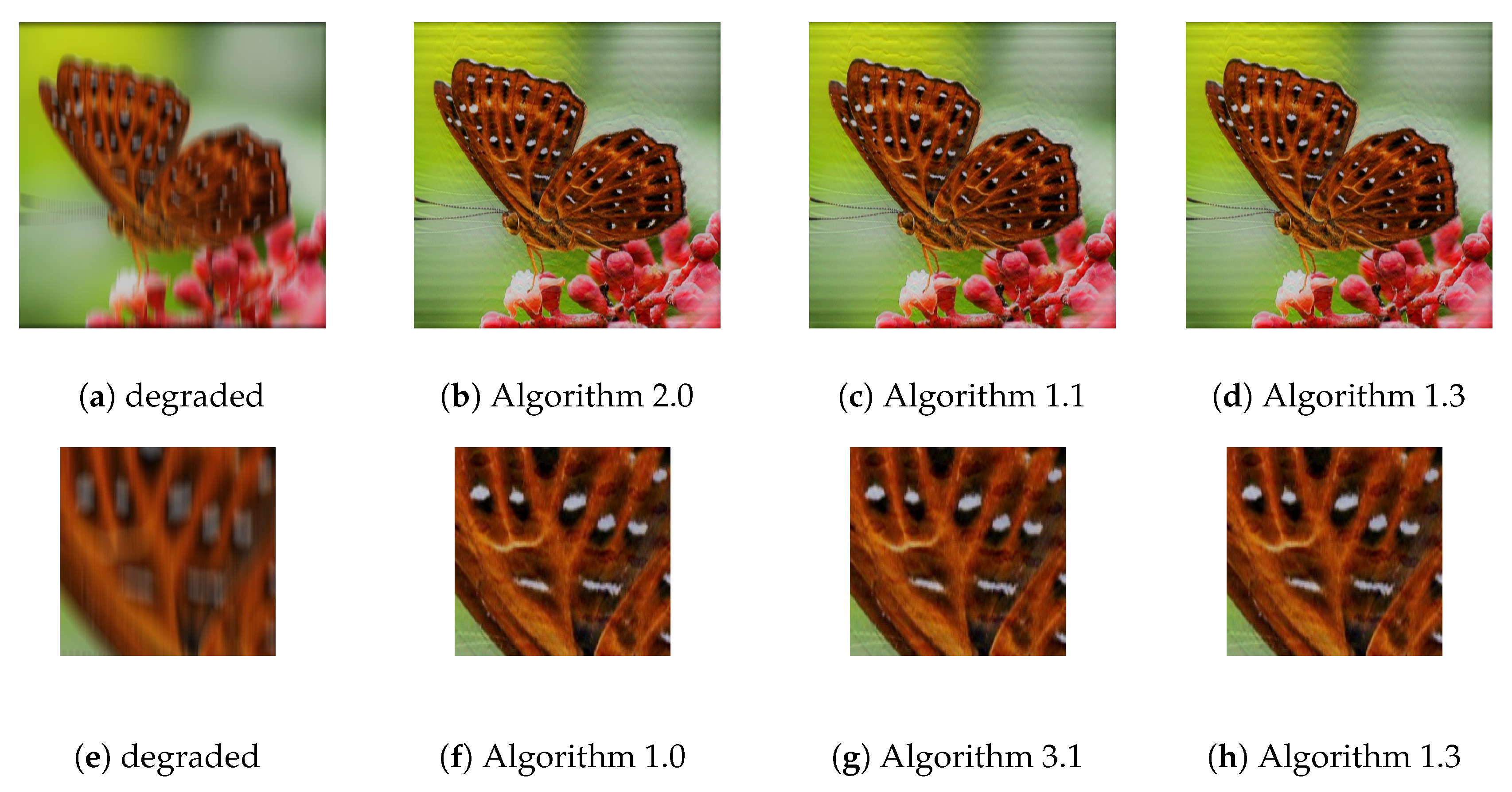
Application to the Image Restoration Problem

The VI problem as mentioned in Section 1 can be applied for solving many problems. Of particular interest, in this subsection, we use Algorithm 1 and Scheme (43) (Algorithm 2) to solve the problem of image deblurring. Furthermore, to illustrate the effectiveness of the proposed scheme, we give a comparative analysis of Algorithm 1 and the algorithms proposed in [49,57]. Furthermore, we compare Scheme 43 with Byrne’s algorithm proposed in [3] for solving the split feasibility problem.

Recall that the image deblurring problem in image processing can be expressed as:

$$c=Mu+\delta ,$$

(44)

where $u\in {\mathbb{R}}^n$ represents the original image, M is the deblurring matrix, c is the observed image, and $\delta \in {\mathbb{R}}^m$ is the Gaussian noise. It has been known that solving (44) is equivalent to solving the convex unconstrained optimization problem:

$$\underset{u\in {\mathbb{R}}^n}{min}\left\{\frac{1}{2}{\parallel Mu-c\parallel }_2^2+\rho {\parallel u\parallel }_1^2\right\},$$

(45)

with $\rho >0$ as the regularization parameter. To solve (45), we suppose $A=\nabla S\left(u\right)$ and $B=\partial T$ where $S\left(u\right)=\frac{1}{2}{\parallel Mu-c\parallel }_2^2$ and $T\left(u\right)={\parallel u\parallel }_1^2,$ then we have that $\nabla S\left(u\right)=M^t(Mu-c)$ is $\frac{1}{{\parallel M\parallel }^2}$-cocoercive. Therefore, for any $0<\tau <\frac{2}{{\parallel M\parallel }^2},$$(I-\tau \nabla S)$ is nonexpansive [58]. The subgradient $\partial T$ is maximal monotone [21]. It is well known that:

$$u\mathrm{is}\mathrm{a}\mathrm{solution}\mathrm{of}\left(45\right)\iff 0\in \nabla S\left(u\right)+\partial T\left(u\right)\iff u=pro{x}_{\rho T}(I-\tau \nabla S)\left(x\right)$$

where $pro{x}_{\rho T}\left(u\right)=argmi{n}_{x\in {\mathbb{R}}^n}\left\{T\left(u\right)+\frac{1}{2\rho }{\parallel u-x\parallel }^2\right\};$ for more details, see [1].

For the split feasibility problem (SFP), we reformulate Problem 45 as a convex constrained optimization problem:

$$\begin{array}{cc}\hfill & \underset{u\in {\mathbb{R}}^n}{min}\frac{1}{2}{\parallel Mu-c\parallel }_2^2\hfill \\ \hfill & {\mathrm{subject}\mathrm{to}\parallel u\parallel }_1\le t,\hfill \end{array}$$

(46)

where $t>0$ is a given constant, and to solve (46), we take $Au=\nabla S\left(u\right)$. We consider $C:=\{u\in {\mathbb{R}}^n:\parallel u{\parallel }_1\le t\}$ and $Q:=\left\{c\right\}.$

To measure the quality of the recovered image, we adopted the improved signal-to-noise ratio (ISNR) [26] and structural similarity index measure (SSIM) [59]. We considered motion blur from MATLAB as the blurring function using (“fspecial(‘motion’,9,40)”). For the comparison, we considered the standard test images of Butterfly $(654\times 654)$, Lena $(512\times 512)$, and Pepper $(512\times 512)$ (see Figure 1). For the control parameters, we took $\varrho =0.9,{\lambda }_0=1,$$\mu =0.3$, and $\rho =0.1,$ for Algorithm 1 and Algorithm 2 (Scheme 43). ${\alpha }_n=0.9$ and ${\lambda }_n=0.5-\frac{150n}{1000n+150}$ for Algorithm $3.1$ in [49], Algorithm $1.3$ in [57], and Algorithm $1.1$ in [3]. For all the algorithms, we took $\frac{\parallel u_{n+1}-u_n{\parallel }_2}{\parallel u_{n+1}{\parallel }_2}<{10}^{-4}$ as the stopping criterion. For reference, all codes were written using MATLAB2018b on a personnel computer.

Figure 1. Original test images. (a) Butterfly, (b) Lena, and (c) Pepper.

It can be seen from Figure 2, Figure 3, Figure 4, Figure 5 and Figure 6 and Table 1 that the recovered images by the proposed Algorithm 1 had higher ISNR and SSIM values, which meant that the quality of the images recovered by Algorithm 1 was better than the compared algorithms.

Figure 2. Degraded and restored (a–d) Butterfly images and (e–h) enlarged Butterfly images by the various algorithms.

Figure 3. Degraded and restored (a–d) Lena images and (e–h) enlarged Lena images by the various algorithms.

Figure 4. Degraded and restored (a–d) Pepper images and (e–h) enlarged Pepper images by the various algorithms.

Figure 5. Degraded and restored (a–c) Butterfly images and (d–f) enlarged Butterfly images by the various algorithms.

Figure 6. Degraded and restored (a–c) Lena images and (d–f) enlarged Lena images by the various algorithms.

Table 1. The ISNR and SSIM values of the compared algorithms.

	Algorithm 1		Moudafi and Oliney		Lorenz and Pock
Images	ISNR	SSIM	ISNR	SSIM	ISNR	SSIM
Butterfly	7.774553	0.9692	7.546909	0.9686	7.587748	0.9688
Lena	7.110084	0.9819	7.126583	0.9813	7.147807	0.9814
Pepper	8.489581	0.9789	8.373034	0.9780	8.354713	0.9779

It can be observed from Figure 5, Figure 6 and Figure 7 that the restoration quality of the images restored by the modified algorithm was better than the quality of the images restored by the compared algorithm, and this is verified by the higher ISNR and SSIM values of Algorithm 2 in Table 2.

Figure 7. Degraded and restored (a–c) Pepper images (d–f) enlarged Pepper images by the various algorithms.

Table 2. The ISNR and SSIM values of the compared algorithms.

	Equation (43)		Byrne
Images	ISNR	SSIM	ISNR	SSIM
Butterfly	7.7741909	0.9999	5.078051	0.9998
Lena	7.112128	0.9999	5.396904	0.9996
Pepper	8.488140	0.9999	6.127068	0.9997

5. Conclusions

A relaxed inertial self-adaptive Tseng-type method for solving the variational inclusion problem was proposed in this work, and the scheme was derived from the explicit time discretization of the dynamical system. The main advantage of this scheme was that it involved both the use of an extrapolation step, as well as a relaxation parameter, and the iterates generated by the proposed scheme converged weakly to the solution of the zeros of the sum of a maximally monotone operator and a monotone operator. Furthermore, the proposed method did not require prior knowledge of the Lipschitz constant of the cost operator, and the iterates generated converged fast to the solution of the problem due to the inertial extrapolation step. A modified scheme derived from the proposed method was given for solving the split feasibility problem. The application of the proposed methods in image recovery and comparison with some of the existing state-of-the-art methods illustrated that the proposed methods are robust and efficient.

References

1. Combettes, P.L.; Wajs, V.R. Signal recovery by proximal forward-backward splitting. Multiscale Model. Simul. 2005, 4, 1168–1200. [Google Scholar] [CrossRef] [Green Version]
2. Byrne, C. A unified treatment of some iterative algorithms in signal processing and image reconstruction. Inverse Probl. 2003, 20, 103. [Google Scholar] [CrossRef] [Green Version]
3. Byrne, C. Iterative oblique projection onto convex sets and the split feasibility problem. Inverse Probl. 2002, 18, 441. [Google Scholar] [CrossRef]
4. Hanjing, A.; Suantai, S. A Fast Image Restoration Algorithm Based on a Fixed Point and Optimization Method. Mathematics 2020, 8, 378. [Google Scholar] [CrossRef] [Green Version]
5. Thong, D.V.; Cholamjiak, P. Strong convergence of a forward–backward splitting method with a new step size for solving monotone inclusions. Comput. Appl. Math. 2019, 38, 94. [Google Scholar] [CrossRef]
6. Marcotte, P. Application of Khobotov’s algorithm to variational inequalities and network equilibrium problems. INFOR Inf. Syst. Oper. Res. 1991, 29, 258–270. [Google Scholar] [CrossRef]
7. Gibali, A.; Thong, D.V. Tseng type methods for solving inclusion problems and its applications. Calcolo 2018, 55, 49. [Google Scholar] [CrossRef]
8. Khobotov, E.N. Modification of the extra-gradient method for solving variational inequalities and certain optimization problems. USSR Comput. Math. Math. Phys. 1987, 27, 120–127. [Google Scholar] [CrossRef]
9. Kinderlehrer, D.; Stampacchia, G. An Introduction to Variational Inequalities and Their Applications; Academic Press: New York, NY, USA, 1980; Volume 31. [Google Scholar]
10. Trémolières, R.; Lions, J.L.; Glowinski, R. Numerical Analysis of Variational Inequalities; North Holland: Amsterdam, The Netherlands, 2011. [Google Scholar]
11. Baiocchi, C. Variational and quasivariational inequalities. In Applications to Free-boundary Problems; Springer: Basel, Switzerland, 1984. [Google Scholar]
12. Konnov, I. Combined Relaxation Methods for Variational Inequalities; Springer Science & Business Media: Berlin/Heidelberg, Germany, 2001; Volume 495. [Google Scholar]
13. Jaiboon, C.; Kumam, P. An extragradient approximation method for system of equilibrium problems and variational inequality problems. Thai J. Math. 2012, 7, 77–104. [Google Scholar]
14. Kumam, W.; Piri, H.; Kumam, P. Solutions of system of equilibrium and variational inequality problems on fixed points of infinite family of nonexpansive mappings. Appl. Math. Comput. 2014, 248, 441–455. [Google Scholar] [CrossRef]
15. Chamnarnpan, T.; Phiangsungnoen, S.; Kumam, P. A new hybrid extragradient algorithm for solving the equilibrium and variational inequality problems. Afrika Matematika 2015, 26, 87–98. [Google Scholar] [CrossRef]
16. Deepho, J.; Kumam, W.; Kumam, P. A new hybrid projection algorithm for solving the split generalized equilibrium problems and the system of variational inequality problems. J. Math. Model. Algorithms Oper. Res. 2014, 13, 405–423. [Google Scholar] [CrossRef]
17. ur Rehman, H.; Kumam, P.; Cho, Y.J.; Yordsorn, P. Weak convergence of explicit extragradient algorithms for solving equilibirum problems. J. Inequal. Appl. 2019, 2019, 1–25. [Google Scholar] [CrossRef]
18. Lions, P.L.; Mercier, B. Splitting algorithms for the sum of two nonlinear operators. SIAM J. Numer. Anal. 1979, 16, 964–979. [Google Scholar] [CrossRef]
19. Passty, G.B. Ergodic convergence to a zero of the sum of monotone operators in Hilbert space. J. Math. Anal. Appl. 1979, 72, 383–390. [Google Scholar] [CrossRef] [Green Version]
20. Tseng, P. A modified forward-backward splitting method for maximal monotone mappings. SIAM J. Control Optim. 2000, 38, 431–446. [Google Scholar] [CrossRef]
21. Rockafellar, R.T. Monotone operators and the proximal point algorithm. SIAM J. Control Optim. 1976, 14, 877–898. [Google Scholar] [CrossRef] [Green Version]
22. Kitkuan, D.; Kumam, P.; Martínez-Moreno, J. Generalized Halpern-type forward–backward splitting methods for convex minimization problems with application to image restoration problems. Optimization 2019, 1–25. [Google Scholar] [CrossRef]
23. Kitkuan, D.; Kumam, P.; Martínez-Moreno, J.; Sitthithakerngkiet, K. Inertial viscosity forward–backward splitting algorithm for monotone inclusions and its application to image restoration problems. Int. J. Comput. Math. 2020, 97, 482–497. [Google Scholar] [CrossRef]
24. Huang, Y.; Dong, Y. New properties of forward–backward splitting and a practical proximal-descent algorithm. Appl. Math. Comput. 2014, 237, 60–68. [Google Scholar] [CrossRef]
25. Goldstein, A.A. Convex programming in Hilbert space. Bull. Am. Math. Soc. 1964, 70, 709–710. [Google Scholar] [CrossRef] [Green Version]
26. Padcharoen, A.; Kitkuan, D.; Kumam, W.; Kumam, P. Tseng methods with inertial for solving inclusion problems and application to image deblurring and image recovery problems. Comput. Math. Method 2020, e1088. [Google Scholar] [CrossRef] [Green Version]
27. Attouch, H.; Peypouquet, J.; Redont, P. Backward–forward algorithms for structured monotone inclusions in Hilbert spaces. J. Math. Anal. Appl. 2018, 457, 1095–1117. [Google Scholar] [CrossRef]
28. Dadashi, V.; Postolache, M. Forward–backward splitting algorithm for fixed point problems and zeros of the sum of monotone operators. Arab. J. Math. 2020, 9, 89–99. [Google Scholar] [CrossRef] [Green Version]
29. Suparatulatorn, R.; Khemphet, A. Tseng type methods for inclusion and fixed point problems with applications. Mathematics 2019, 7, 1175. [Google Scholar] [CrossRef] [Green Version]
30. Bauschke, H.H.; Combettes, P.L. Convex Analysis and Monotone Operator Theory in Hilbert Spaces; Springer: New York, NY, USA, 2011; Volume 408. [Google Scholar]
31. Eckstein, J.; Bertsekas, D.P. On the Douglas—Rachford splitting method and the proximal point algorithm for maximal monotone operators. Math. Program. 1992, 55, 293–318. [Google Scholar] [CrossRef] [Green Version]
32. Polyak, B.T. Some methods of speeding up the convergence of iteration methods. USSR Comput.Math. Math. Phys. 1964, 4, 1–17. [Google Scholar] [CrossRef]
33. Nesterov, Y. A method for unconstrained convex minimization problem with the rate of convergence O (1/k2). Doklady Ussr 1983, 269, 543–547. [Google Scholar]
34. Alvarez, F. On the minimizing property of a second order dissipative system in Hilbert spaces. SIAM J. Control Optim. 2000, 38, 1102–1119. [Google Scholar] [CrossRef] [Green Version]
35. Alvarez, F.; Attouch, H. An inertial proximal method for maximal monotone operators via discretization of a nonlinear oscillator with damping. Set-Valued Anal. 2001, 9, 3–11. [Google Scholar] [CrossRef]
36. Dong, Q.; Cho, Y.; Zhong, L.; Rassias, T.M. Inertial projection and contraction algorithms for variational inequalities. J. Glob. Optim. 2018, 70, 687–704. [Google Scholar] [CrossRef]
37. Abubakar, J.; Sombut, K.; Ibrahim, A.H. An Accelerated Subgradient Extragradient Algorithm for Strongly Pseudomonotone Variational Inequality Problems. Thai J. Math. 2019, 18, 166–187. [Google Scholar]
38. Van Hieu, D. An inertial-like proximal algorithm for equilibrium problems. Math. Methods Oper. Res. 2018, 1–17. [Google Scholar] [CrossRef]
39. Thong, D.V.; Van Hieu, D. Inertial extragradient algorithms for strongly pseudomonotone variational inequalities. J. Comput. Appl. Math. 2018, 341, 80–98. [Google Scholar] [CrossRef]
40. Abubakar, J.; Kumam, P.; Rehman, H.; Ibrahim, A.H. Inertial Iterative Schemes with Variable Step Sizes for Variational Inequality Problem Involving Pseudomonotone Operator. Mathematics 2020, 8, 609. [Google Scholar] [CrossRef]
41. Attouch, H.; Cabot, A. Convergence of a relaxed inertial proximal algorithm for maximally monotone operators. Math. Program. 2019. [Google Scholar] [CrossRef]
42. Attouch, H.; Cabot, A. Convergence rate of a relaxed inertial proximal algorithm for convex minimization. Optimization 2019. [Google Scholar] [CrossRef]
43. Attouch, H.; Cabot, A. Convergence of a Relaxed Inertial Forward–Backward Algorithm for Structured Monotone Inclusions. Appl. Math. Optim. 2019, 80, 547–598. [Google Scholar] [CrossRef]
44. Boţ, R.I.; Csetnek, E.R.; Hendrich, C. Inertial Douglas–Rachford splitting for monotone inclusion problems. Appl. Math. Comput. 2015, 256, 472–487. [Google Scholar] [CrossRef] [Green Version]
45. Iutzeler, F.; Hendrickx, J.M. A generic online acceleration scheme for optimization algorithms via relaxation and inertia. Optim. Methods Softw. 2019, 34, 383–405. [Google Scholar] [CrossRef] [Green Version]
46. Alves, M.M.; Marcavillaca, R.T. On inexact relative-error hybrid proximal extragradient, forward-backward and Tseng’s modified forward-backward methods with inertial effects. Set-Valued Variat. Anal. 2019, 1–25. [Google Scholar] [CrossRef] [Green Version]
47. Alves, M.M.; Eckstein, J.; Geremia, M.; Melo, J.G. Relative-error inertial-relaxed inexact versions of Douglas-Rachford and ADMM splitting algorithms. Comput. Optim. Appl. 2020, 75, 389–422. [Google Scholar] [CrossRef] [Green Version]
48. Xia, Y.; Wang, J. A general methodology for designing globally convergent optimization neural networks. IEEE Trans. Neural Netw. 1998, 9, 1331–1343. [Google Scholar] [PubMed] [Green Version]
49. Lorenz, D.A.; Pock, T. An inertial forward-backward algorithm for monotone inclusions. J. Math. Imaging Vis. 2015, 51, 311–325. [Google Scholar] [CrossRef] [Green Version]
50. Takahashi, W. Nonlinear Functional Analysis-Fixed Point Theory and its Applications; Springer: New York, NY, USA, 2000. [Google Scholar]
51. Brezis, H. Ope Rateurs Maximaux Monotones Et Semi-Groupes De Contractions Dans Les Espaces De Hilbert; Elsevier: North Holland, The Netherlands, 1973. [Google Scholar]
52. Ofoedu, E. Strong convergence theorem for uniformly L-Lipschitzian asymptotically pseudocontractive mapping in real Banach space. J. Math. Anal. Appl. 2006, 321, 722–728. [Google Scholar] [CrossRef] [Green Version]
53. Opial, Z. Weak convergence of the sequence of successive approximations for nonexpansive mappings. Bull. Am. Math. Soc. 1967, 73, 591–597. [Google Scholar] [CrossRef] [Green Version]
54. Censor, Y.; Elfving, T. A multiprojection algorithm using Bregman projections in a product space. Numer. Algorithms 1994, 8, 221–239. [Google Scholar] [CrossRef]
55. Censor, Y.; Elfving, T.; Kopf, N.; Bortfeld, T. The multiple-sets split feasibility problem and its applications for inverse problems. Inverse Probl. 2005, 21, 2071. [Google Scholar] [CrossRef] [Green Version]
56. Censor, Y.; Bortfeld, T.; Martin, B.; Trofimov, A. A unified approach for inversion problems in intensity-modulated radiation therapy. Phys. Med. Biol. 2006, 51, 2353. [Google Scholar] [CrossRef] [Green Version]
57. Moudafi, A.; Oliny, M. Convergence of a splitting inertial proximal method for monotone operators. J. Comput. Appl. Math. 2003, 155, 447–454. [Google Scholar] [CrossRef] [Green Version]
58. Iiduka, H.; Takahashi, W. Strong convergence theorems for nonexpansive nonself-mappings and inverse-strongly-monotone mappings. J. Convex Anal. 2004, 11, 69–79. [Google Scholar]
59. Wang, Z.; Bovik, A.C.; Sheikh, H.R.; Simoncelli, E.P. Image quality assessment: From error visibility to structural similarity. IEEE Trans. Image Process. 2004, 13, 600–612. [Google Scholar] [CrossRef] [Green Version]