Abstract
We study the global asymptotic stability problem with respect to the fractional-order quaternion-valued bidirectional associative memory neural network (FQVBAMNN) models in this paper. Whether the real and imaginary parts of quaternion-valued activation functions are expressed implicitly or explicitly, they are considered to meet the global Lipschitz condition in the quaternion field. New sufficient conditions are derived by applying the principle of homeomorphism, Lyapunov fractional-order method and linear matrix inequality (LMI) approach for the two cases of activation functions. The results confirm the existence, uniqueness and global asymptotic stability of the system’s equilibrium point. Finally, two numerical examples with their simulation results are provided to show the effectiveness of the obtained results.
1. Introduction
Recently, many analyses pertaining to the dynamical behaviors of different classes of neural network (NN) models have been reported in the literature. The results of NNs have been successfully applied to a variety of domains, which include pattern recognition, artificial intelligence, optimal control, signal processing, and other engineering problems [1,2,3,4,5,6]. In all these applications, the investigation on the stability of the NN models is of paramount importance. Among different NN models, the bidirectional associative memory (BAM) model is another kind of recurrent NNs [7]. The BAM NN model is a two-layer, nonlinear feedback network model, and it has formulated that the neurons in one layer are always interconnected to neurons in another layer, which has been widely used because of their mathematical modeling capabilities. As a result, BAM NN models have received significant research attention in both areas of the field of both mathematical and practical analysis [8,9,10,11,12,13,14,15].
On the other hand, due to their extensive applications of NNs in science and engineering disciplines, real-valued neural networks (RVNNs) and complex-valued neural networks (CVNNs) have been successfully analyzed by many researchers [10,11,16,17,18,19,20,21,22,23,24,25]. In recent years, various NNs have been studied in multi-dimensional space with much interest. While both RVNNs and CVNNs are helpless when implementing and data into NNs directly. As such, quaternion-valued neural networks (QVNNs) has been developed by implementing quaternion algebra into NNs in order to generalize both CVNNs and RVNNs [26,27,28]. Recent research shows that QVNNs can effectively deal with and data and have found their successful application in color image processing, and wind forecasting, body motion tracking, computer graphics, optimization, polarized signal classification, molecular modeling [29,30,31,32,33,34]. The main advantage of the QVNN model is its capability of reducing computational complexity in multi-dimensional problems. Recently, several studies on various dynamics of QVNN models have been studied [35,36,37,38,39,40,41,42,43,44]. By the use of Halanay inequality and matrix measure methods, sufficient conditions for the global exponential stability of the unique equilibrium state have been obtained in Reference [35]. Based on new Lyapunov functional and some inequality techniques, global synchronization conditions were derived for fractional-order QVNNs in Reference [36]. The issue of global -stability of QVNNs was studied in Reference [38]. In Reference [40], the problem of global Mittag-Leffler stability and stabilization has been investigated for fractional-order quaternion-valued memristive NNs by using the real-imaginary separate method. The fractional-order QVNN model was analyzed in Reference [41], in which issues related to synchronization and global Mittag-Leffler stability were tackled. Based on the geometric properties of the activation functions, the multistability issue for delayed QVNNs was studied in Reference [43]. In References [44,45], by employing the direct quaternion method, the problem of stability and stabilization analysis for QVNNs has been studied. Many similar outcomes can be found in the literature, for example, References [13,37,39,40,42].
It is known that fractional calculus mainly deals with derivatives and integrals of arbitrary non-integer order. Recently, fractional calculus has been shown as a powerful methodology for modeling many physical and engineering processes include mechanics, chemistry, biology, and image processing. The main topics include vibration and control, continuous-time random walk, Levy statistics, power law, Riesz potential, nonlocal phenomena, biomedical engineering, and so on [46,47,48]. In comparison with the integer-order model, the primary benefit of fractional-order model is two aspects; one is its infinite memory, the other is the parameter of the fractional-order enriching systems output by increasing a degree of freedom. Comparing with integer order calculus, fractional-order derivatives offer a variety of merits to represent properties with respect to real-world memory and hereditary. As such, the Caputo, Riemann-Liouville as well as Atangana-Baleanu fractional derivatives have attracted much attention [47,48,49]. Recently, fractional-order NN models have received substantial research attention in both mathematical and practical analysis [12,13,14,50,51,52,53]. As an example, by use of new fractional-order inequality as well as the Lyapunov fractional-order method, the global Mittag-Leffler synchronization problem pertaining to FQVBAMNN models was studied in Reference [13]. In Reference [14], the quasi-pinning synchronization of BAM fractional-order NN models was analyzed with discontinuous neuron activations. To reduce the complexity in calculations of fractional-order QVNNs, the decomposition method was used to the problem of finite-time Mittag-Leffler stability in Reference [52]. On the other hand, only a few works are reported in the dynamical analysis of FQVBAMNNs. According to our survey, the FQVBAMNNs are new to the study on the global asymptotic stability analysis and our article contributes to this area of research.
Inspired by the above discussions, our analysis focuses on the global asymptotic stability problem for the FQVBAMNN models. Throughout this study, whether the real and imaginary parts of quaternion-valued activation functions are expressed implicitly or explicitly, they are considered to meet the global Lipschitz condition in the quaternion field. By using the homeomorphism principle, Lyapunov fractional-order method and LMI approach, new sufficient conditions for the two types of activation functions are derived. The results confirm the existence, uniqueness, and global asymptotic stability of the system’s equilibrium point. We use two examples to illustrate the feasibility and benefits of the obtained results. The main contributions of this paper can be listed as follows: (1) results regarding the stability of FQVBAMNN is limited. This paper contributes to analyzing this research area, and global asymptotic stability also investigated. (2) quaternion-valued LMI is equivalently translated into real-valued LMI, which can easily be checked by the LMI toolbox in Matlab. (3) the obtained main results are more concise and new compared to the previous results.
Notations: The sets of quaternion, complex, and real numbers are denoted by , , and , respectively. Their matrices are denoted by , while their and n dimensional vectors are denoted by , , , respectively. In addition, the diagonal of a block diagonal matrix is denoted as ; a positive (negative) definite matrix of is denoted as ; while the identity matrix is denoted as . The matrix transposition and conjugate transpose and matrix transposition are denoted as superscript T and *, respectively. Finally, given the block of a quaternion matrix, its conjugate transpose is denoted as ★, while ✠ indicates the symmetric terms in a matrix.
2. Formulation of the Problem and Fundamentals
2.1. Quaternion Algebra
Firstly, we address the quaternion and its operating rules. Quaternion is generally represented in the form as
where ; the imaginary roots satisfy the following Hamilton multiplication rules:
The operations between quaternions and are defined as follows. The addition and subtraction of quaternions are defined as
The module for a quaternion , denoted by , is defined as
where represents the conjugate transpose of z. The norm of z is defined as .
2.2. Caputo Fractional-Order Derivative
We give the definition of Euler’s gamma function as
Definition 1
([47]). The fractional-order of Caputo derivative of order for a function is defined as
where is the initial time and n is the positive integer such that , and . is gamma function.
Definition 2
([47]). The Riemann-Liouville fractional integral of is defined as
2.3. Problem Formulation
We consider a class of FQVBAMNN models in this section, as follows:
or an equivalent vector form:
where the external input vectors are denoted as , ; the vector-valued activation functions are denoted as , ; the state vectors are denoted as and . While with with are the self-feedback connection weight matrices; are the connection weight matrices.
Remark 1.
Recently, several approaches have been taken into consideration to study complex-valued type of activation functions [13,15,18,19,40,44,45,54]. The two main approaches are—either to express the activation function into two parts (real and imaginary) parts [13,15,40,54], or keep the activation function intact without separation into real and imaginary parts [18,19,44,45]. Accordingly, the following assumptions are established.
Assumption 1.
The neuron activation functions of and , satisfy the following Lipschitz condition:
where and are positive constants.
Based on Assumption 1, we have
where and .
Assumption 2.
For and with . The neuron activation functions and can be separated into real and imaginary parts as
where . In addition, the following conditions are satisfied by both the real and imaginary parts:
(1) Given variables , , , , the partial derivatives of and exist, and they are continuous.
(2) All the partial derivatives are bounded, that is, there exist positive constant numbers , , , , , , , , , , , , , , , , , , , , , , , , , , , , , , , such that
As a result, we have the following inequalities
holds for any , , , . Moreover , for all .
2.4. Fundamentals
For the analysis of the main results, the following lemmas are required.
Lemma 1
([53]). Let any be continuous and differentiable, it implies that for any matrix ,
Lemma 2
([54]). For any vectors , and , the following condition is true: .
Lemma 3
([45]). For any vectors , and , the following condition is true: .
Lemma 4
([15]). A continuous map is denoted as , and it satisfies
(i) is injective on ,
(ii) as , then H is homeomorphism of onto itself.
Lemma 5
([55]). A continuous map is denoted as , and it satisfies
(i) is injective on ,
(ii) as , then is homeomorphism of onto itself.
Lemma 6
([45]). A continuous map is denoted as , and it satisfies
(i) is injective on ,
(ii) as , then is homeomorphism of onto itself.
Lemma 7
([3]). Given , where . As such, is equivalent to one of the following conditions
Lemma 8
([45]). Gien , where . As such, is equivalent to one of the following conditions
Lemma 9
([45]). Let be a Hermitian matrix. As such, is equivalent to
Remark 2.
Unlike real and complex numbers, the commutative principle is not satisfied by quaternion multiplication. Therefore, methods and techniques for analysis of CVNN or RVNN models cannot be directly applied to QVNN models. A straightforward way to perform analysis on the QVNN model is to exploit the Hamilton rules with respect to the non-commutative quaternion multiplication, that is, separating a QVNN model into either (i) four RVNN models; or (ii) two CVNN models, for further analysis.
3. Main Results
In this section, subject to Assumption 1, we will derive new sufficient conditions with respect to the existence, uniqueness, and global asymptotic stability pertaining to the equilibrium point for the NN model in (3).
3.1. Real-Imaginary Separate-Type Activation Functions
By applying the quaternion multiplication, (7) can be expressed as:
Let
The equivalent form of the model in (8) is
With respect to Assumption 1, we have
where , .
Note that the NN models in (3) and (9) have the same equilibrium point, indicating that both models have the same stability condition. Therefore, based on the inequality (12), the existence, uniqueness, and global asymptotic stability of its equilibrium point are analyzed for the NN model (9).
Theorem 1.
Consider the real-imaginary separate-type activation functions, which satisfy Assumption 1. Given the NN model in (9), its equilibrium point is globally asymptotically stable subject to the existence of scalars and matrices in such a way that the following LMI is met:
Proof.
First, we show the existence and uniqueness of the equilibrium point for NN (9). A map associated with the model in (9) is defined as follows.
Next, it is possible to prove that the map is injective through contradiction. Suppose that there exist whereby .
According to (13), we have
If (13) holds, by Schur complement, we have
As such, the right-hand side of (21) is negative, and this presents a contradiction. As a result, the map is injective.
Then, it is possible to prove that as . Based on (21), we obtain
subject to a sufficiently small ; as such, we have
One can infer from (24) that
Therefore, as . Based on Lemma 4, we can see that the map is homeomorphic on . As a result, a unique point exists whereby . In other words, a unique equilibrium point exists for the model in (9).
By transformation of , , we can shift the equilibrium point pertaining to the model in (9) to the origin. We then have
where , and .
Remark 3.
Theorem 1 provides sufficient conditions for the existence, uniqueness and global asymptotic stability of the NN model by splitting the real-imaginary separate type activation function. If it is not possible to split the activation function into real-imaginary parts, the results obtained in Theorem 1 are invalid. Next, we analyze the NN model in (3) under the condition that the activation functions cannot be divided into real-imaginary separate types.
3.2. The Activation Functions Cannot Be Expressed through Separation of the Real and Imaginary Parts
Theorem 2.
With respect to Assumption 1, consider the scenario that it is unable to separate the activation functions into real and imaginary parts. As such, the model in (3) has an equilibrium point that is globally asymptotically stable, subject to the existence of scalars and Hermitian matrices , whereby the following LMI is satisfied:
where
Proof.
Given the NN model in (3), we show the existence and uniqueness of its equilibrium point. A map associated with the model in (3) is defined as follows
Similarly, it is possible to prove that the map is injective through contradiction. Suppose that there exist whereby . According to (33), we have
If (33) holds, by Schur complement, we have
As such, the right-hand side of (41) is negative, and this presents a contradiction. As a result, the map is injective.
Then, it is possible to prove that as . Based on (41), we obtain
Subject to a sufficiently small ; as such, we have
One can infer from (44) that
Therefore, as . Based on Lemma 6, we can see that the map is homeomorphic on . As a result, a unique point exists whereby . In other words, a unique equilibrium point exists for the model in (3).
By transformation of , , we can shift the equilibrium point pertaining to the NN model in (3) to the origin. Then, we have
where , and .
We use the following Lyapunov functional to ascertain the global asymptotic stability with respect to the equilibrium point pertaining to the model in (46),
where and . As such, we obtain the following from the time derivative of with respect to the solution of (46)
By using the Shcur complement lemma, we have
Using Lemma 9, if , , such that
where are defined in Theorem 2.
Remark 4.
It is known that QVNN models are the generalization of CVNN and RVNN models. As such, the global asymptotic stability criterion for both CVNN and RVNN models can be obtained by using the same methods as in Theorems 1 and 2.
Consider a CVNN model with the following form. We have
where the external input vectors are denoted as , ; the connection weight matrix and delayed connection weight matrix are denoted as and ; the self-feedback connection weight positive diagonal matrices are denoted as and ; the vector-valued activation functions are denoted as , ; the state vectors are denoted as and ; and .
We can express he model in (55) in accordance with the definition of complex numbers as follows
By applying complex multiplication, we can express (55) as
Let
Assumption 3.
The functions and are continuous and satisfy the following Lipschitz condition
where and are constants.
As such, the models in (58) and (55) have the same equilibrium point. Similarly, the stability of models (58) and (55) is equivalent.
Corollary 1.
Consider the activation functions which cannot be expressed through separation into the real-imaginary parts, and which satisfy Assumption 1. Given the model in (55), its equilibrium point is globally asymptotically stable subject to the existence of scalars and Hermitian matrices , in such a way that the following LMI is met:
where
Remark 5.
In QVNN analysis, the quaternion-valued LMI can not verify directly in Matlab LMI. In Theorem 16, how the quaternion-valued LMI can be resolved easily is well stated. By the use fo proposed Lemma in [40,55], the quaternion-valued LMI is equivalently translated into real-valued LMI, which can easily be checked by the LMI toolbox in Matlab.
4. Illustrative Examples
In this section, two numerical examples are given to illustrate the usefulness of the derived results.
Example 1.
We consider an FQVBAMNN model with two neurons, as follows:
We can conclude that , . Under simple calculation, from (62) we can obtain directly , , and . It is possible to verify the LMI conditions in (13) with the MATLAB LMI software package. The following feasible solutions can be obtained by solving Theorem 1 with and and
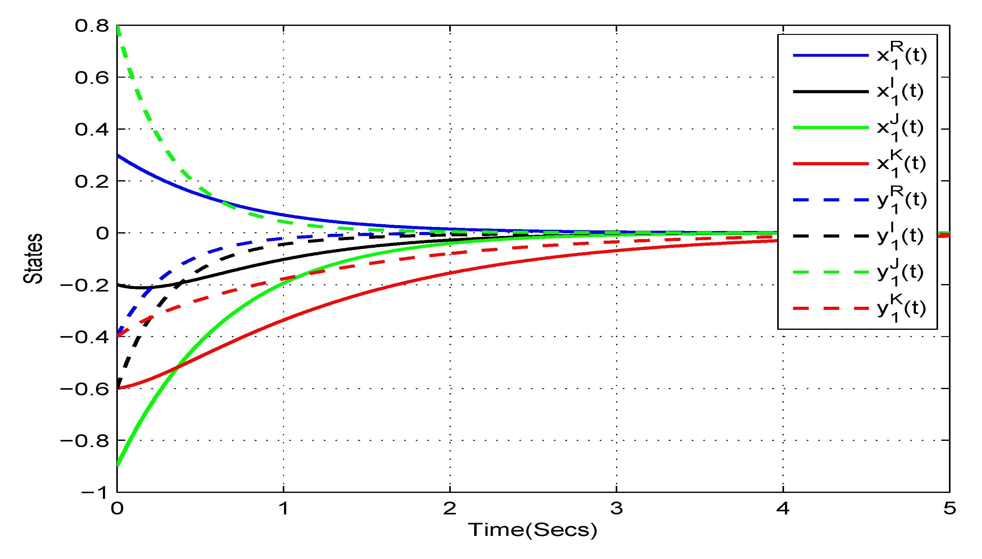
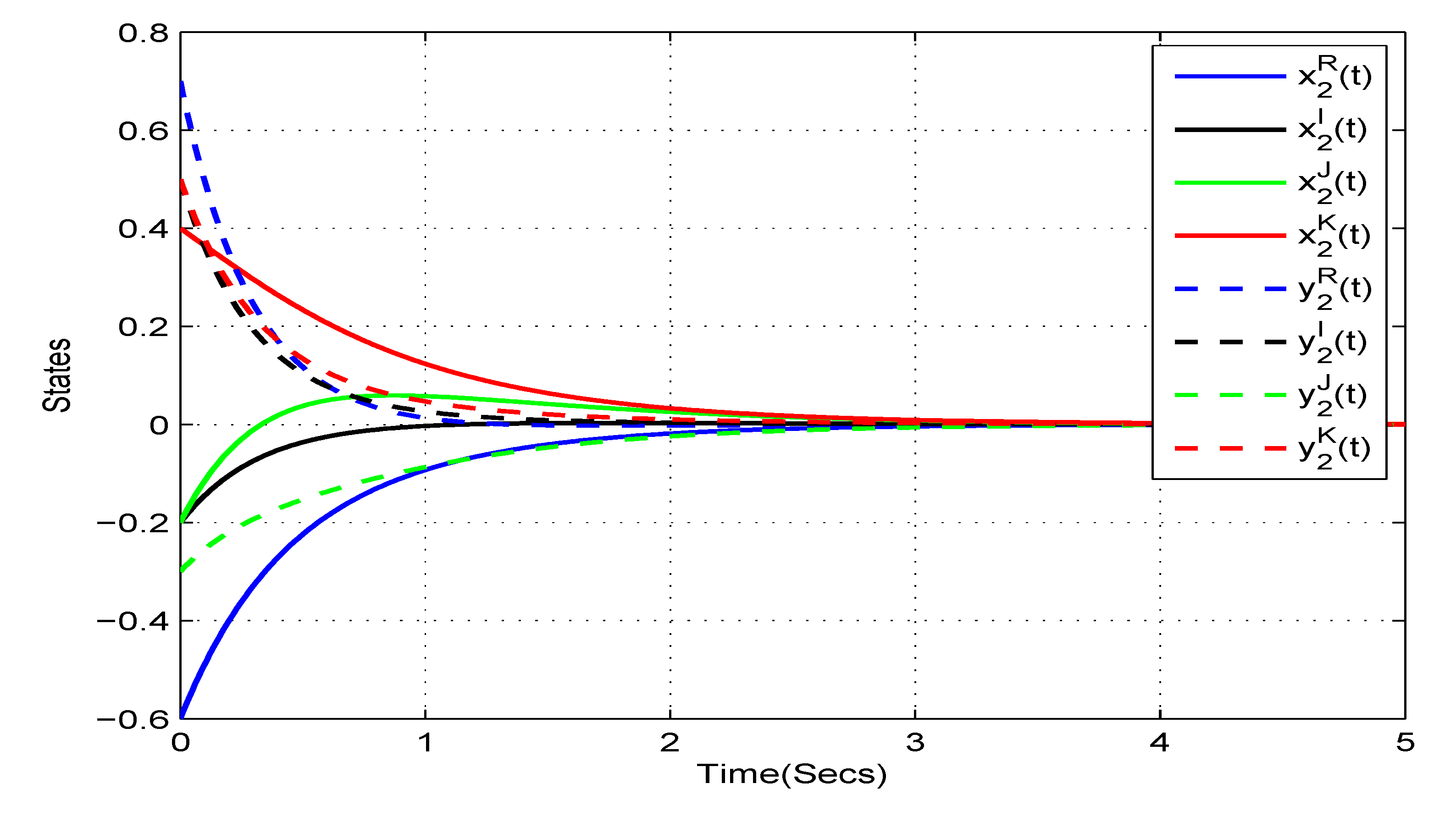
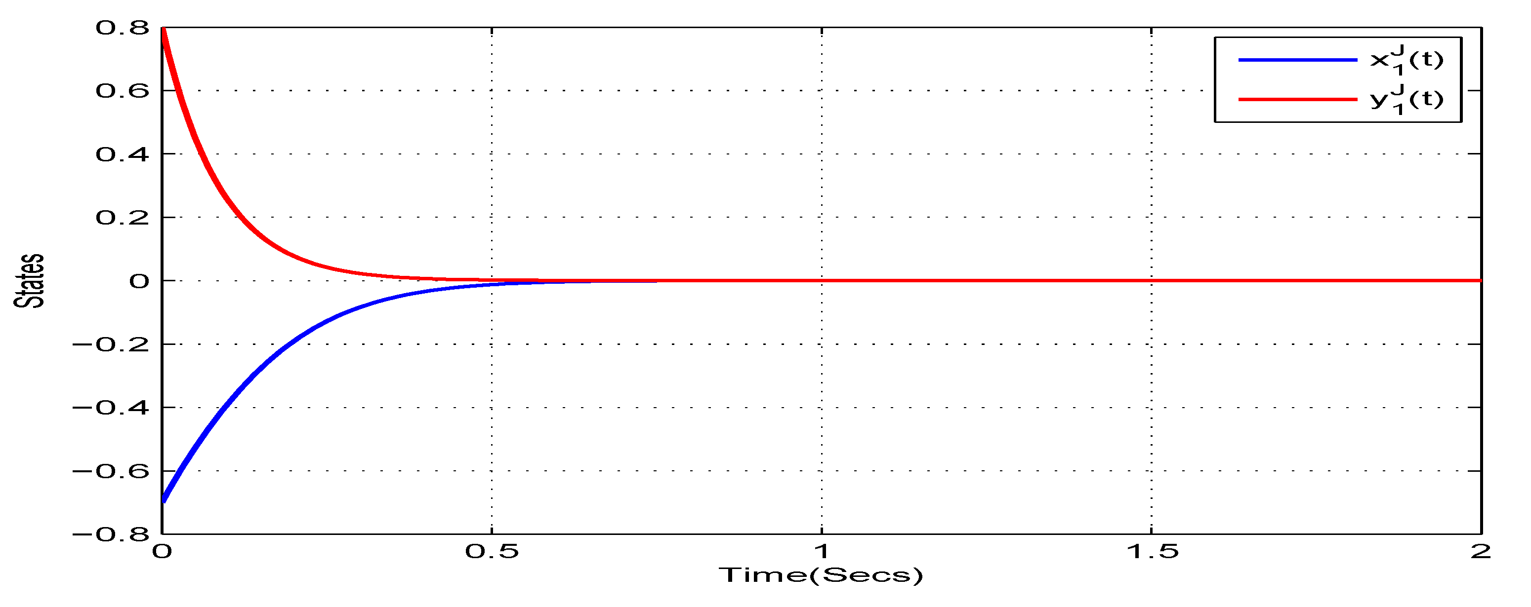
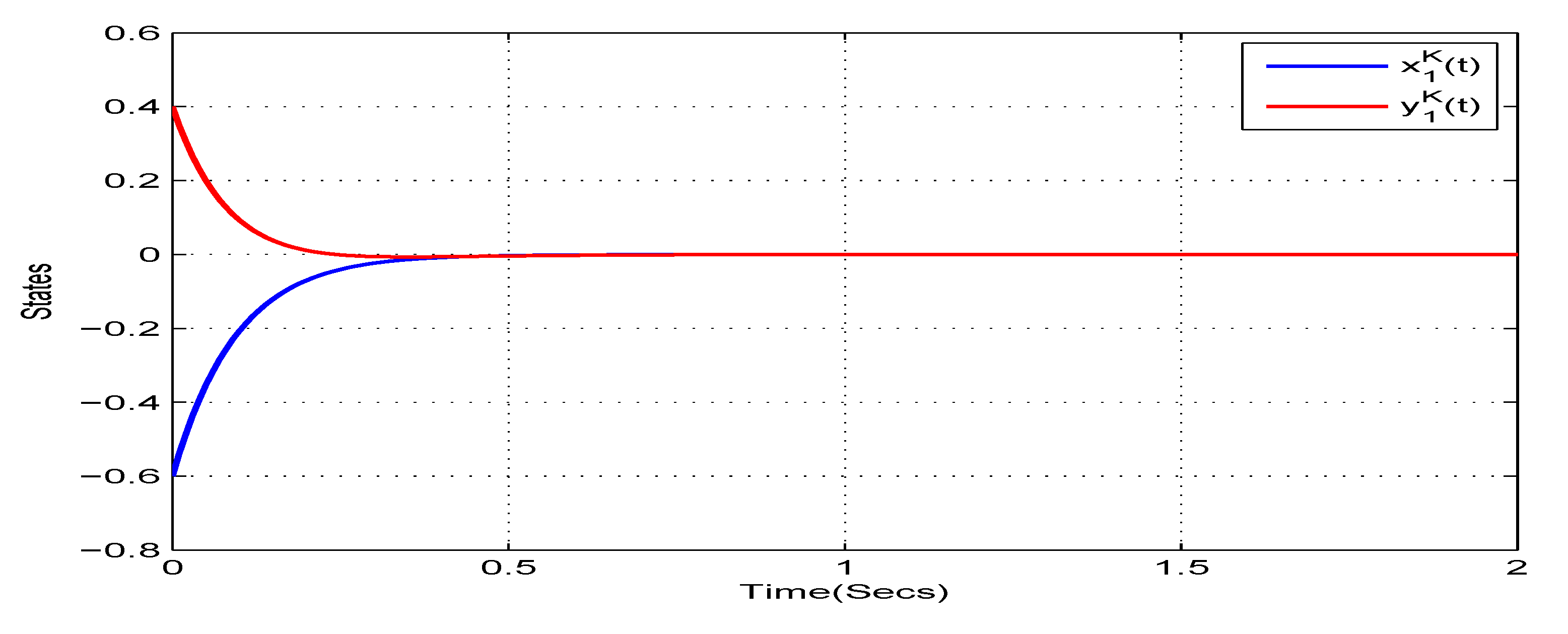
The activation functions are assumed to be . Figure 1 depicts the time responses with respect to states of the real and imaginary parts of , , , , subject to the initial states of , , and . Figure 2 depicts the time responses with respect to the states of , , , , subject to the same initial conditions. From these Figure 1 and Figure 2, we can see that the state trajectories of the NN model (62) converge to the equilibrium point. According to Theorem 1, we can conclude the FQVBAMNN model is globally asymptotically stable.
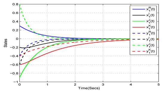
Figure 1.
An illustration of the time responses with respect to the real-imaginary parts pertaining to the states of , , , in Example 1.
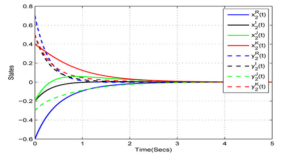
Figure 2.
An illustration of the time responses with respect to the real-imaginary parts pertaining to the states of , , , in Example 1.
Example 2.
We consider an FQVBAMNN model with two neurons, as follows:
We can conclude that , . The LMI condition in (33) can be verified with the MATLAB LMI software package. The following feasible solutions can be obtained with and ,
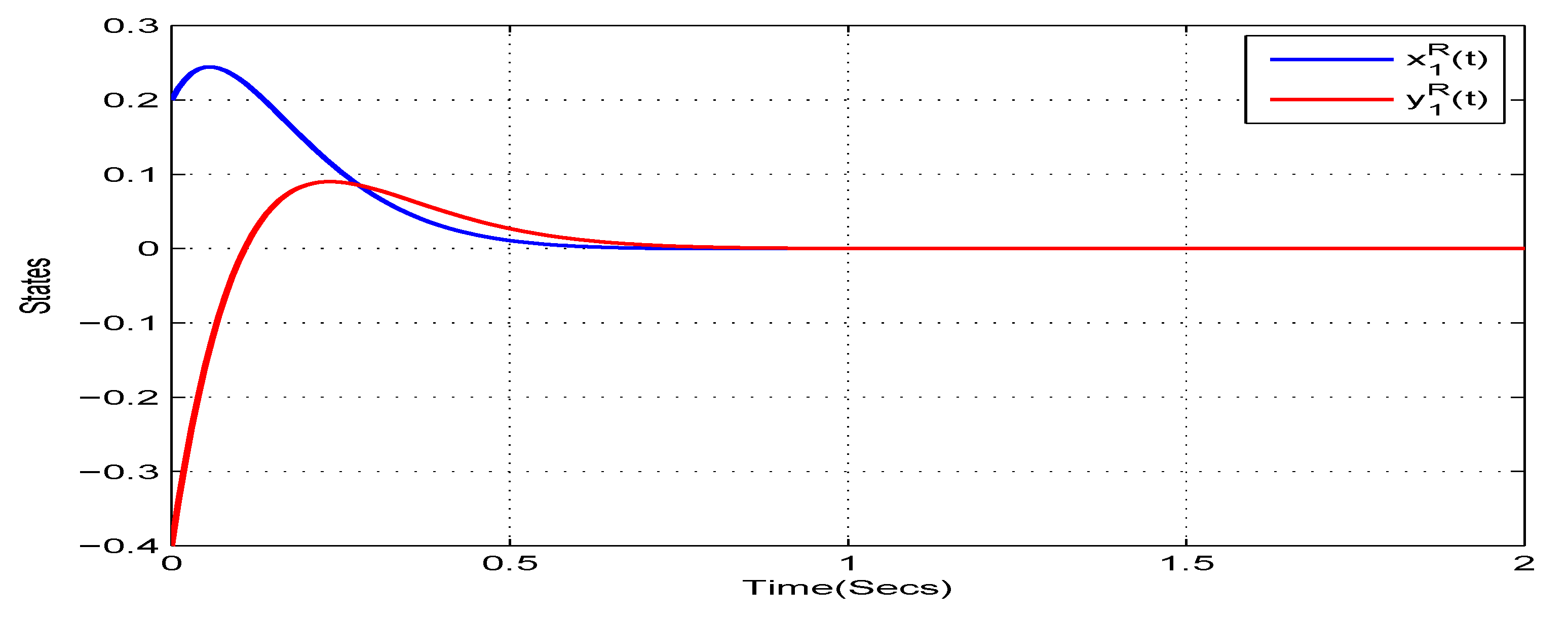
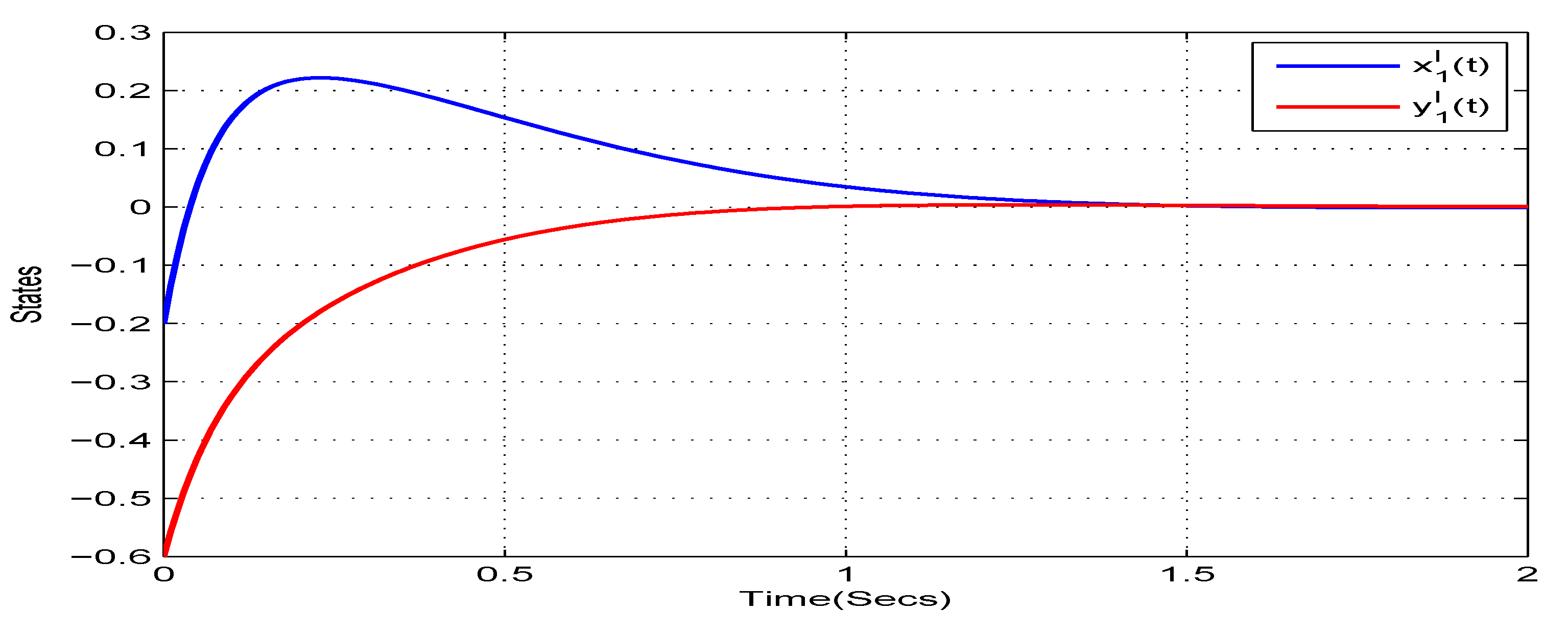
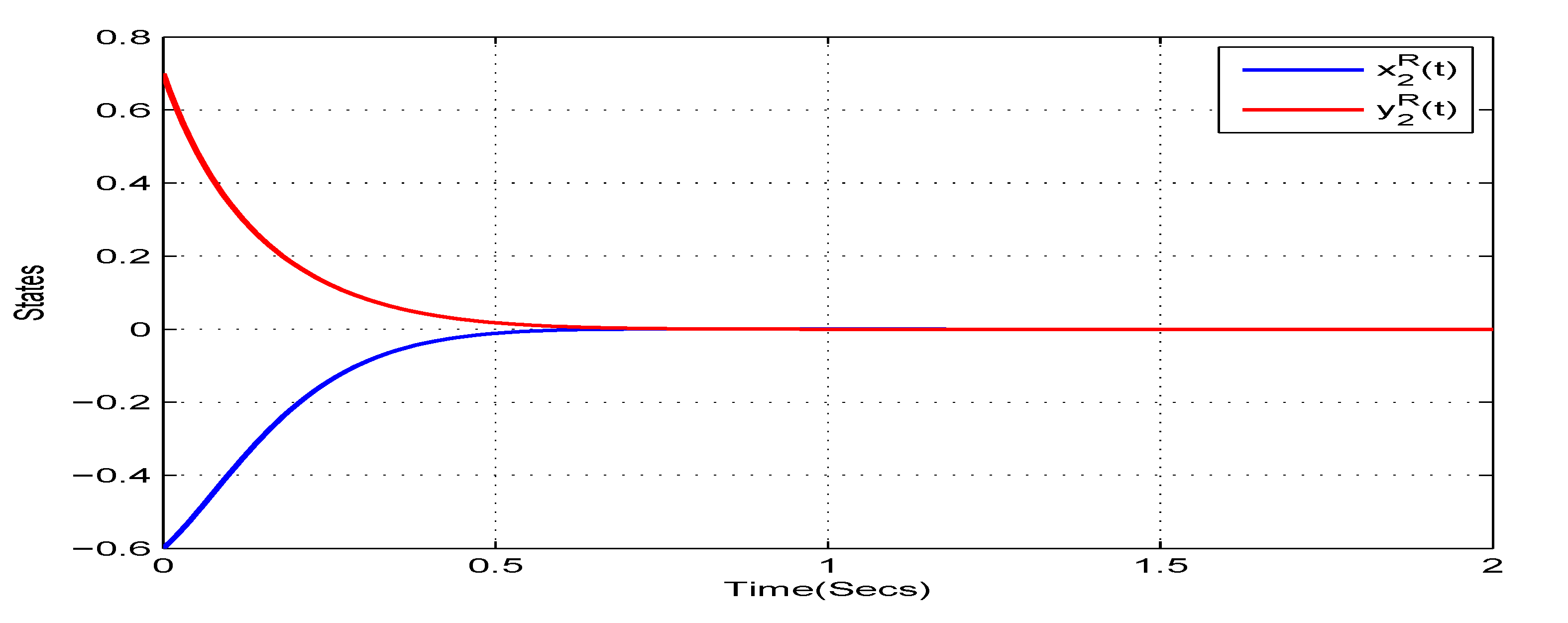
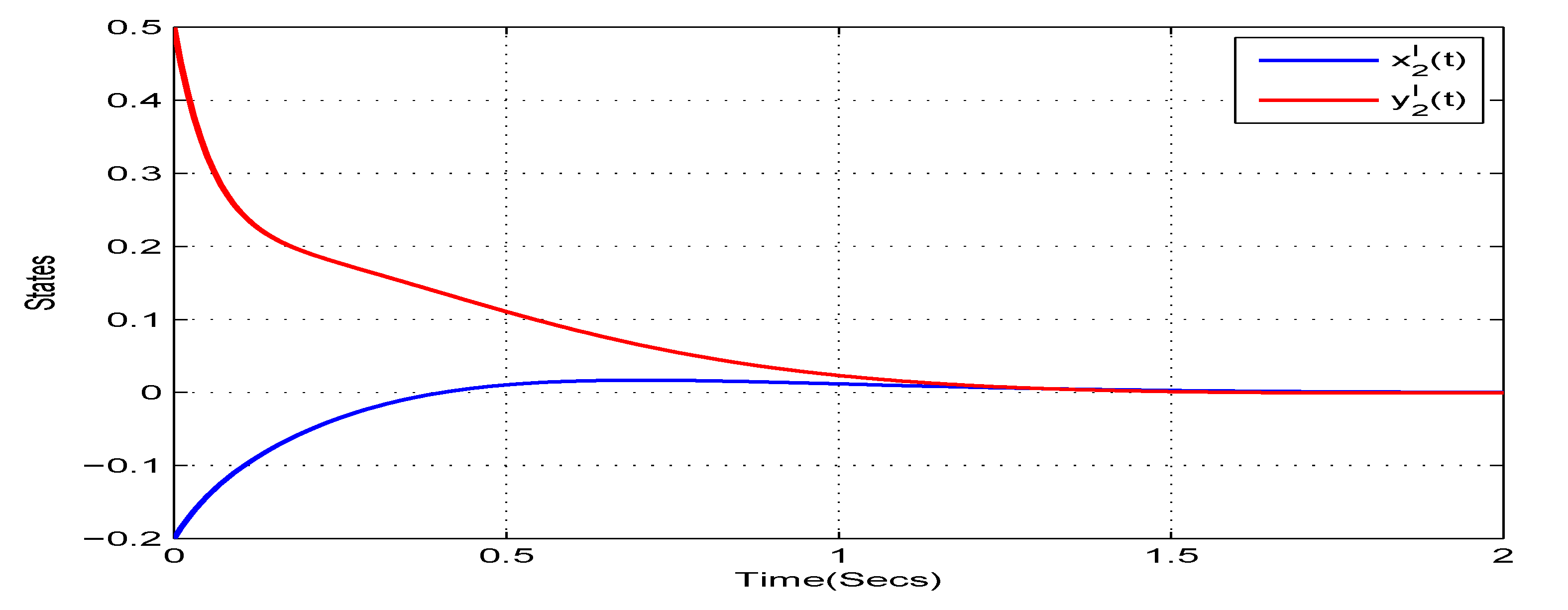
The activation functions are assumed to be , . Besides, the initial conditions are chosen to be , , and . Figure 3, Figure 4, Figure 5, Figure 6, Figure 7, Figure 8, Figure 9 and Figure 10 depict the time responses with respect to the real-imaginary parts pertaining to the states of , , , , , , , . From these Figure 3, Figure 4, Figure 5, Figure 6, Figure 7, Figure 8, Figure 9 and Figure 10, we can see that the state trajectories of the NN model (63) converge to the equilibrium point. According to Theorem 2, we can conclude the FQVBAMNN model is globally asymptotically stable.

Figure 3.
An illustration of the time responses with respect to the real part pertaining to the states of in Example 2.

Figure 4.
An illustration of the time responses with respect to the imaginary part pertaining to the states of in Example 2.
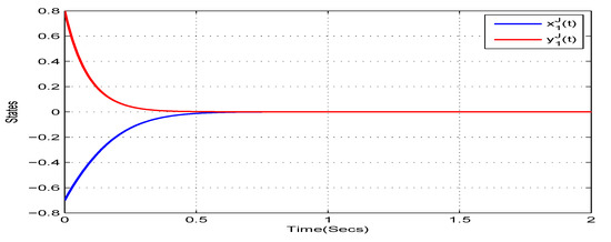
Figure 5.
An illustration of the time responses with respect to the imaginary part pertaining to the states of in Example 2.
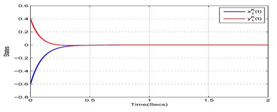
Figure 6.
An illustration of the time responses with respect to the imaginary part pertaining to the states of in Example 2.

Figure 7.
An illustration of the time responses with respect to the imaginary part pertaining to the states of in Example 2.
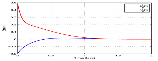
Figure 8.
An illustration of the time responses with respect to the imaginary part pertaining to the states of in Example 2.
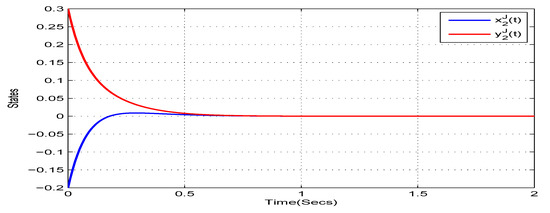
Figure 9.
An illustration of the time responses with respect to the imaginary part pertaining to the states of in Example 2.
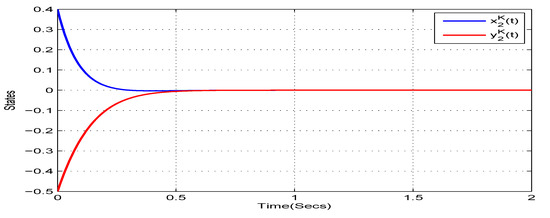
Figure 10.
The time responses for the imaginary parts of the states in Example 2.
5. Conclusions
In this research, we have investigated the FQVBAMNN models with respect to its existence, uniqueness and global asymptotic stability. Whether or not the quaternion-valued activation functions are expressed directly by dividing real and imaginary parts, which always presumed to meet the globally Lipschitz condition in the quaternion field. New sufficient conditions are derived by applying the principle of homeomorphism, Lyapunov fractional-order method and LMI approach for the two cases of activation functions, which ensure the existence, uniqueness, and globally asymptotic stability of the equilibrium point of the considered system model. Finally, two numerical examples and their simulation results are provided to show the effectiveness of the results.
Based on the results presented in this paper, it is possible to analyze different QVNN models. The proposed methods can be extended to study uncertain, stochastic, as well as discrete-time QVNN models. We also intend to examine the different types of stability analysis, which include robust stability and finite-time stability, with respect to discrete-time QVNN models. The results will be useful for the dynamical analysis of discrete-time QVNN models.
Author Contributions
Conceptualization, G.R.; Formal analysis, G.R.; Funding acquisition, U.H.; Investigation, G.R.; Methodology, G.R.; Resources, G.R.; Software, P.K., P.C., R.S. (Ramalingam Sriraman) and R.S. (Rajendran Samidurai); Supervision, C.P.L.; Validation, G.R.; Writing—original draft, G.R.; Writing—review & editing, G.R. All authors have read and agreed to the published version of the manuscript.
Funding
This research is made possible through financial support of King Mongkut’s University of Technology Thonburi (KMUTT) and the Thailand research Grant Fund (RSA6280004).
Acknowledgments
The authors acknowledge King Mongkut’s University of Technology Thonburi for funding Postdoctoral Fellowship to Pramet Kaewmesri and the Thailand research Grant Fund (RSA6280004). The authors are very grateful to the Department of Mathematics, Faculty of Science, King Mongkut’s University of Technology Thonburi (KMUTT) for all support.
Conflicts of Interest
The authors declare no conflict of interest.
References
- Feng, C.; Plamondon, R. On the stability analysis of delayed neural networks systems. Neural Netw. 2001, 14, 1181–1188. [Google Scholar] [CrossRef]
- Kwon, O.M.; Lee, S.M.; Park, J.H.; Cha, E.J. New approaches on stability criteria for neural networks with interval time-varying delays. Appl. Math. Comput. 2012, 218, 9953–9964. [Google Scholar] [CrossRef]
- Kwon, O.M.; Park, J.H. New delay-dependent robust stability criterion for uncertain neural networks with time-varying delays. Appl. Math. Comput. 2008, 205, 417–427. [Google Scholar] [CrossRef]
- Liu, L.; Deng, F. Stability analysis of time-varying delayed stochastic Hopfield neural networks in numerical simulation. Neurocomputing 2018, 316, 294–305. [Google Scholar] [CrossRef]
- Wang, T.; Zhao, S.; Zhou, W.; Yu, W. Finite-time state estimation for delayed Hopfield neural networks with Markovian jump. Neurocomputing 2015, 156, 193–198. [Google Scholar] [CrossRef]
- Samidurai, R.; Sriraman, R. Robust dissipativity analysis for uncertain neural networks with additive time-varying delays and general activation functions. Math. Comput. Simulat. 2019, 155, 201–216. [Google Scholar] [CrossRef]
- Kosko, B. Adaptive bidirectional associative memories. Appl. Opt. 1987, 26, 4947–4960. [Google Scholar] [CrossRef]
- Wang, G.; Cao, J.; Xu, M. Stability analysis for stochastic BAM neural networks with Markovian jumping parameters. Neurocomputing 2009, 72, 3901–3906. [Google Scholar] [CrossRef]
- Li, X. Exponential stability of Cohen-Grossberg-type BAM neural networks with time-varying delays via impulsive control. Neurocomputing 2009, 73, 525–530. [Google Scholar] [CrossRef]
- Liu, B.W. Global exponential stability for BAM neural networks with time-varying delays in the leakage terms. Nonlinear Anal. Real World Appl. 2013, 14, 559–566. [Google Scholar] [CrossRef]
- Wang, T.; Zhu, Q. Stability analysis of stochastic BAM neural networks with reaction-diffusion, multi-proportional and distributed delays. Phys. A Stat. Mech. Appl. 2019, 533, 121935. [Google Scholar] [CrossRef]
- Bao, H.; Park, J.H.; Cao, J. Non-fragile state estimation for fractional-order delayed memristive BAM neural networks. Neural Netw. 2019, 119, 190–199. [Google Scholar] [CrossRef] [PubMed]
- Xiao, J.; Wen, S.; Yang, X.; Zhong, S. New approach to global Mittag-Leffler synchronization problem of fractional-order quaternion-valued BAM neural networks based on a new inequality. Neural Netw. 2020, 122, 320–337. [Google Scholar] [CrossRef] [PubMed]
- Pratap, A.; Raja, R.; Cao, J.; Rihan, F.A.; Seadawy, A.R. Quasi-pinning synchronization and stabilization of fractional-order BAM neural networks with delays and discontinuous neuron activations. Chaos Soliton. Fract. 2020, 131, 109491. [Google Scholar] [CrossRef]
- Wang, Z.; Huang, L. Global stability analysis for delayed complex-valued BAM neural networks. Neurocomputing 2016, 173, 2083–2089. [Google Scholar] [CrossRef]
- Wang, Z.; Guo, Z.; Huang, L.; Liu, X. Dynamical behavior of complex-valued Hopfield neural networks with discontinuous activation functions. Neural Process. Lett. 2017, 45, 1039–1061. [Google Scholar] [CrossRef]
- Sriraman, R.; Samidurai, R. Global asymptotic stability analysis for neutral-type complex-valued neural networks with random time-varying delays. Int. J. Syst. Sci. 2019, 50, 1742–1756. [Google Scholar] [CrossRef]
- Samidurai, R.; Sriraman, R.; Cao, J.; Tu, Z. Effects of leakage delay on global asymptotic stability of complex-valued neural networks with interval time-varying delays via new complex-valued Jensen’s inequality. Int. J. Adapt. Control Signal Process. 2018, 32, 1294–1312. [Google Scholar] [CrossRef]
- Tu, Z.; Cao, J.; Alsaedi, A.; Alsaadi, F.E.; Hayat, T. Global Lagrange stability of complex-valued neural networks of neutral type with time-varying delays. Complexity 2016, 21, 438–450. [Google Scholar] [CrossRef]
- Gunasekaran, N.; Zhai, G. Stability analysis for uncertain switched delayed complex-valued neural networks. Neurocomputing 2019, 367, 198–206. [Google Scholar] [CrossRef]
- Gunasekaran, N.; Zhai, G. Sampled-data state-estimation of delayed complex-valued neural networks. Int. J. Syst. Sci. 2020, 51, 303–312. [Google Scholar] [CrossRef]
- Zhang, W.; Cao, J.; Chen, D.; Alsaadi, F.E. Synchronization in fractional-order complex-valued delayed neural networks. Entropy 2018, 20, 54. [Google Scholar] [CrossRef]
- Li, L.; Wang, Z.; Lu, J.; Li, Y. Adaptive synchronization of fractional-order complex-valued neural networks with discrete and distributed delays. Entropy 2018, 20, 124. [Google Scholar] [CrossRef]
- Nitta, T. Solving the XOR problem and the detection of symmetry using a single complex-valued neuron. Neural Netw. 2003, 16, 1101–1105. [Google Scholar] [CrossRef]
- Goh, S.L.; Chen, M.; Popovic, D.H.; Aihara, K.; Obradovic, D.; Mandic, D.P. Complex-valued forecasting of wind profile. Renew. Energy 2006, 31, 1733–1750. [Google Scholar] [CrossRef]
- Hamilton, W.R. On quaternions. Proc. R. Ir. Acad. 1847, 3, 1–16. [Google Scholar]
- Zhang, F. Quaternions and matrices of quaternions. Linear Algebra Appl. 1997, 251, 21–57. [Google Scholar] [CrossRef]
- Matsui, N.; Isokawa, T.; Kusamichi, H. Quaternion neural network with geometrical operators. J. Intell. Fuzzy Syst. 2004, 15, 149–164. [Google Scholar]
- Isokawa, T.; Kusakabe, T.; Matsui, N.; Peper, F. Quaternion neural networks and its application. In International Conference on Knowledge-Based and Intelligent Information and Engineering Systems; LNAI-2774 (KES2003); Springer: Berlin/Heidelberg, Germany, 2003; pp. 318–324. [Google Scholar]
- Karney, C.F.F. Quaternions in molecular modeling. J. Mol. Graphics Model. 2007, 25, 595–604. [Google Scholar] [CrossRef]
- Bolboacă, S.D.; Jäntschi, L. Helical structure of linear homopolymers. Mater. Res. Proc. 2018, 8, 35–51. [Google Scholar]
- Buchholz, S.; Le Bihan, N. Polarized signal classification by complex and quaternionic multi-layer perceptrons. Int. J. Neural Syst. 2008, 18, 75–85. [Google Scholar] [CrossRef] [PubMed]
- Marques, J.M.C.; Pereira, F.B.; Llanio-Trujillo, J.L.; Abreu, P.E.; Alberti, M.; Aguilar, A.; Pirani, F.; Bartolomei, M. A global optimization perspective on molecular clusters. Philos. Trans. R. Soc. A 2017, 375, 20160198. [Google Scholar] [CrossRef] [PubMed]
- Jäntschi, L.; Bolboacă, S.D. Conformational study of C-24 cyclic polyyne clusters. Int. J. Quantum Chem. 2018, 118, e25614. [Google Scholar] [CrossRef]
- Liu, Y.; Zhang, D.; Lu, J. Global exponential stability for quaternion-valued recurrent neural networks with time-varying delays. Nonlinear Dyn. 2017, 87, 553–565. [Google Scholar] [CrossRef]
- Li, H.L.; Jiang, H.; Cao, J. Global synchronization of fractional-order quaternion-valued neural networks with leakage and discrete delays. Neurocomputing 2020, 385, 211–219. [Google Scholar] [CrossRef]
- Liu, J.; Jian, J. Global dissipativity of a class of quaternion-valued BAM neural networks with time delay. Neurocomputing 2019, 349, 123–132. [Google Scholar] [CrossRef]
- You, X.; Song, Q.; Liang, J.; Liu, Y.; Alsaadi, F.E. Global μ-stability of quaternion-valued neural networks with mixed time-varying delays. Neurocomputing 2018, 290, 12–25. [Google Scholar] [CrossRef]
- Xiao, J.; Zhong, S. Synchronization and stability of delayed fractional-order memristive quaternion-valued neural networks with parameter uncertainties. Neurocomputing 2019, 363, 321–338. [Google Scholar] [CrossRef]
- Rajchakit, G.; Chanthorn, P.; Kaewmesri, P.; Sriraman, R.; Lim, C.P. Global Mittag-Leffler stability and stabilization analysis of fractional-order quaternion-valued memristive neural networks. Mathematics 2020, 8, 422. [Google Scholar] [CrossRef]
- Yang, X.; Li, C.; Song, Q.; Chen, J.; Huang, J. Global Mittag-Leffler stability and synchronization analysis of fractional-order quaternion-valued neural networks with linear threshold neurons. Neural Netw. 2018, 105, 88–103. [Google Scholar] [CrossRef]
- Qi, X.; Bao, H.; Cao, J. Exponential input-to-state stability of quaternion-valued neural networks with time delay. Appl. Math. Comput. 2019, 358, 382–393. [Google Scholar] [CrossRef]
- Song, Q.; Chen, X. Multistability analysis of quaternion-valued neural networks with time delays. IEEE Trans. Neural Netw. Learn. Syst. 2018, 12, 5430–5440. [Google Scholar] [CrossRef] [PubMed]
- Tu, Z.; Zhao, Y.; Ding, N.; Feng, Y.; Zhang, W. Stability analysis of quaternion-valued neural networks with both discrete and distributed delays. Appl. Math. Comput. 2019, 343, 342–353. [Google Scholar] [CrossRef]
- Tu, Z.; Yang, X.; Wang, L.; Ding, N. Stability and stabilization of quaternion-valued neural networks with uncertain time-delayed impulses: Direct quaternion method. Phys. A Stat. Mech. Appl. 2019, 535, 122358. [Google Scholar] [CrossRef]
- Oldham, K.B.; Spanier, J. The Fractional Calculus; Academic Press: New York, NY, USA, 1974. [Google Scholar]
- Podlubny, I. Fractional Differential Equations; Academic Press: San Diego, CA, USA, 1999. [Google Scholar]
- Kilbas, A.A.; Srivastava, H.M.; Trujillo, J.J. Theory and Applications of Fractional Differential Equations; Elsevier: Amsterdam, The Netherlands, 2006. [Google Scholar]
- Syam, M.I.; Al-Refai, M. Fractional differential equations with Atangana-Baleanu fractional derivative: Analysis and applications. Chaos Soliton. Fract. 2019, 2, 100013. [Google Scholar] [CrossRef]
- Pratap, A.; Raja, R.; Cao, J.; Rajchakit, G.; Lim, C.P. Global robust synchronization of fractional order complex-valued neural networks with mixed time-varying delays and impulses. Int. J. Control. Autom. Syst. 2019, 17, 509–520. [Google Scholar]
- Bao, H.; Park, J.H.; Cao, J. Synchronization of fractional-order complex-valued neural networks with time delay. Neural Netw. 2016, 81, 16–28. [Google Scholar] [CrossRef]
- Pratap, A.; Raja, R.; Alzabut, J.; Dianavinnarasi, J.; Cao, J.; Rajchakit, G. Finite-time Mittag-Leffler stability of fractional-order quaternion-valued memristive neural networks with impulses. Neural Process. Lett. 2020, 51, 1485–1526. [Google Scholar] [CrossRef]
- Camacho, N.A.; Duarte-Mermoud, M.A.; Gallegos, J.A. Lyapunov-functions for fractional order systems. Commun. Nonlinear Sci. Numer. Simul. 2014, 19, 2951–2957. [Google Scholar] [CrossRef]
- Zhang, Z.; Liu, X.; Chen, J.; Guo, R.; Zhou, S. Further stability analysis for delayed complex-valued recurrent neural networks. Neurocomputing 2017, 251, 81–89. [Google Scholar] [CrossRef]
- Subramanian, K.; Muthukumar, P. Existence, uniqueness and global asymptotic stability analysis for delayed complex-valued Cohen-rossberg BAM neural networks. Neural Comput. Appl. 2018, 29, 565–584. [Google Scholar] [CrossRef]
© 2020 by the authors. Licensee MDPI, Basel, Switzerland. This article is an open access article distributed under the terms and conditions of the Creative Commons Attribution (CC BY) license (http://creativecommons.org/licenses/by/4.0/).

