Unsteady Three-Dimensional MHD Non-Axisymmetric Homann Stagnation Point Flow of a Hybrid Nanofluid with Stability Analysis

Abstract

The hybrid nanofluid under the influence of magnetohydrodynamics (MHD) is a new interest in the industrial sector due to its applications, such as in solar water heating and scraped surface heat exchangers. Thus, the present study accentuates the analysis of an unsteady three-dimensional MHD non-axisymmetric Homann stagnation point flow of a hybrid Al₂O₃-Cu/H₂O nanofluid with stability analysis. By employing suitable similarity transformations, the governing mathematical model in the form of the partial differential equations are simplified into a system of ordinary differential equations. The simplified mathematical model is then solved numerically by the Matlab solver bvp4c function. This solving approach was proficient in generating more than one solution when good initial guesses were provided. The numerical results presented significant influences on the rate of heat transfer and fluid flow characteristics of a hybrid nanofluid. The rate of heat transfer and the trend of the skin friction coefficient improve with the increment of the nanoparticles’ concentration and the magnetic parameter; however, they deteriorate when the unsteadiness parameter increases. In contrast, the ratio of the escalation of the ambient fluid strain rate to the plate was able to adjourn the boundary layer separation. The dual solutions (first and second solutions) are obtainable when the surface of the sheet shrunk. A stability analysis is carried out to justify the stability of the dual solutions, and hence the first solution is seen as physically reliable and stable, while the second solution is unstable.

1. Introduction

The stagnation point flow has attracted vast attention from many researchers because of its broad applications in both industrial and scientific applications. Some of the real-world applications of the stagnation point flow lie in the polymer industry, extrusion processes, plane counter-jets, and numerous forms of hydrodynamic modelling in engineering uses ([1,2,3]). An exact solution of the steady two-dimensional stagnation-point flow towards a solid surface in moving fluid was first discovered by Hiemenz [4] in 1911. In his particular study, the Navier–Stokes equations are reduced to non-linear ordinary differential equations by using a similarity transformation. The remarkable work done by Hiemenz [4] was extended by Homann [5], who started the classical work of three-dimensional stagnation point flow for the axisymmetric case. Meanwhile, the flow in the neighbourhood of a particular stagnation point on a surface was explored by Howarth [6], focusing on the non-axisymmetric three-dimensional flow near the stagnation region. Fast forward to 1961, the work of Howarth [6] was criticized by Davey [7], who indicated a mistake in Howarth’s paper exposing that the results in the region $-1\le c\le 0$ are unable to be achieved from those discovered for $0\le c\le 1$ as reported in the study. In conjunction with these findings, Davey and Schofield [8] initiated the study of these saddle point solutions and justified the existence of the non-uniqueness solution. In another study, Weidman [9] modified the Homann’s axisymmetric outer potential stagnation-point flow for non-axisymmetric stagnation flow of the strain rate. The study revealed a new clan of asymmetric viscous stagnation point flows liable on the shear rate ratio, $\gamma =b/a$ where $-\infty \le \gamma \le \infty$, $a$ is the strain rate and $b$ is the shear rate. An analysis of unsteady heat transmission in non-axisymmetric Homann stagnation-point flows of a viscous fluid over a rigid plate was investigated by Mahapatra and Sidui [10], and recently, an investigation on the non-axisymmetric Homann stagnation-point flows of a viscoelastic fluid towards a fixed plate was conducted by Mahapatra and Sidui [11].

Ever since the evolution study of the stagnation point flow with the presence of dual solutions by Davey [7], various works concerning the stagnation point flow towards a shrinking sheet were introduced. Wang [12] considered two-dimensional stagnation point flow on a two-dimensional shrinking sheet and axisymmetric stagnation point flow on an axisymmetric shrinking sheet, while Mahapatra and Sidui [13] assessed unsteady heat transfer in non-axisymmetric Homann stagnation-point flow towards a stretching/shrinking sheet with stability analysis. The continuous effort was carried out by Khashi’ie et al. [14] who examined the three-dimensional non-axisymmetric Homann stagnation point flow and heat transfer past a stretching/shrinking sheet using hybrid nanofluid. Meanwhile, Zaimi and Ishak [15] scrutinized the slip effects on the stagnation point flow towards a stretching vertical sheet. Nevertheless, explorations on the stagnation point flow keep evolving in various ways and have been working still because of its importance in massive engineering applications and also in the magnetohydrodynamics (MHD) flow field. A comprehensive study of the literature on the related works was reviewed by [16,17,18,19].

A fluid that is heated by electric energy in the occurrence of a vigorous magnetic field, such as crystal growth in melting, is essential in the industrial sector. The interaction of electrical currents and magnetic fields generates the divergence of Lorentz forces during the movement of fluid. In accordance with this phenomenon, MHD describes the hydrodynamics of a conducting fluid in the presence of a magnetic field. The examinations of MHD flow are very significant due to its massive number of uses implicating the magnetic effect in industrial and engineering areas, such as MHD electricity generators, sterilization tools, magnetic resonance graphs, MHD flow meters, and also in granular insulation (see [20,21]). The goods of the end product depend immensely on the rate of cooling involved in these processes, managed by the application of the magnetic field and electrically conducting fluids. The study of MHD flow in the Newtonian fluid was first carried out by Pavlov [22], who investigated the magnetohydrodynamic flow of an impressible viscous fluid caused by deformation of a surface. Chakrabarti and Gupta [23] broadened the study of hydromagnetic flow and heat transfer over a stretching sheet, followed by Vajravelu [24] who widened the hydromagnetic flow study over a continuous, moving, porous flat surface. Andersson, in 1995, introduced an exact solution of the Navier-Stokes equations for magnetohydrodynamic flow [25], and Lok et al. [26] analyzed the MHD stagnation-point flow towards a shrinking sheet using the Keller-box method and proved the existence of multiple (dual) solutions for small values of the magnetic field parameter for the shrinking case. Recently, Almutairi et al. [27] studied the influence of second-order velocity slip on the MHD flow of a nanofluid in a porous medium by considering the homogeneous-heterogeneous reactions. On the other hand, the impact of nonlinear and temperature jump on non-Newtonian MHD nanofluid flow and heat transfer past a stretched thin sheet was examined by Zhu et al. [28]

Over the last few decades, the researcher has experienced tremendous scholarly devotion to the study of heat transfer fluid. Recent demand for a high-efficiency refrigeration system and the ineffectiveness of traditional thermal conduction fluids encouraged analysts to discover another heat transfer fluid. Choi and Eastman [29] launched the exploration of nanofluids and illustrated the presence of suspended nanoparticles in a carrier fluid. This pioneering study led to the verdict of the colloidal suspension of intensely small-sized particles, for instance, carbon nanotubes, metals, oxides, and carbides, into the based fluid, which may ensure access to an advanced course of nanotechnology-based heat transfer media (see [30,31]). The eccentric features of nanofluids have gained great acknowledgement in various engineering, medical, and industrial applications like engine cooling, diesel generator efficiency, micro-manufacturing, solar water heating, cancer treatment, nuclear reactors, and diverse types of heat exchangers ([32,33,34]). Due to the massive potential for the applications of nanofluids, Choi and Eastmen [29] developed a mathematical model of nanofluids, which allowed Buongiorno [31] to contribute to heat transfer analysis in nanofluids by introducing the non-homogeneous model for transport and heat transfer phenomena in nanofluids with turbulence applications.

Recently, an expansion of new engineered nanofluids was achieved by dispersing composite nanopowder or dissimilar nanoparticles with sizes between 1 and 10nm in the base fluid [29]; it is known as a hybrid nanofluid. The hybrid nanofluid is a modern technology fluid that may offer better heat transfer performance and thermal physical properties. The progress related to the preparation methods of hybrid nanofluids, thermo-physical properties of hybrid nanofluids, and current applications of hybrid nanofluids was published by Sarkar et al. [35] and Sidik et al. [36]. In another study, Huminic and Huminic [37] highlighted the essential applications of hybrid nanofluids, such as in heat pipes, mini-channel heat sinks, plate heat exchangers, air conditioning systems, tubular heat exchangers, shell and tube heat exchangers, tube in a tube heat exchangers, and coiled heat exchangers. Turcu et al. [38], for the first time testified the hybrid nanocomposite particle synthesis, which consisted of two different hybrids, polypyrrole-carbon nanotube (PPY-CNT) nanocomposite and multi-walled carbon nanotube (MWCNT) on magnetic Fe₃O₄ nanoparticles. In the following year, Yen et al. [39] inspected the effect of hybrid nanofluids in channel flow numerically. Devi and Devi [40] analysed the problem of hydromagnetic hybrid nanofluid (Cu-Al₂O₃/water) flow on a permeable stretching sheet subject to Newtonian heating, and they continued the investigation to improve the heat transfer in hybrid nanofluid flow past a stretching sheet [41]. Subsequently, Yousefi et al. [42] reviewed on the stagnation point flow of an aqueous titania-copper hybrid nanofluid toward a wavy cylinder. At the same time, Khashi’ie et al. [43] performed a numerical study on the heat transfer and boundary layer flow of axisymmetric hybrid nanofluids driven by a stretching/shrinking disc. A detailed documentary on the numerical study of hybrid nanofluid flow and heat transfer is reviewed by [44,45,46,47,48].

Many practical situations, such as a sudden stretching of the plate or temperature change of the plate, involved unsteady conditions of the heat transfer flow. Cai et al. [49] explained that the flow in the viscous boundary layer near the plate would slowly be enlarged if the surface was extended unexpectedly, and hence converted into a steady flow after a certain interval. Technically, we believe that the consideration of physical quantities related to time is crucial in mathematical modeling and analysis, which is acknowledged in the formulation of this research problem.

Motivated by the work by Mahapatra and Sidui [13], this study aims to inspect the unsteady MHD non-axisymmetric Homann stagnation point of a hybrid nanofluid in three-dimensional flow. The proposed hybrid nanofluid model is adapted from Devi and Devi [40] and Hayat and Nadeem [50], recognized by suspending varied nanoparticles, namely alumina (Al₂O₃) and copper (Cu), in the base fluid (water). To the best of the authors’ knowledge, no attempt has been made to examine the heat transfer and fluid flow of the hybrid nanofluid (Al₂O₃-Cu/H₂O) considering the unsteady parameter in non-axisymmetric Homann stagnation point flow. This possibly will benefit future works on choosing a significant parameter to enhance the heat transfer performance in the modern industry. The novelty of this study can also be seen in the discovery of dual solutions and the execution of stability analysis. Ultimately, this research is highly claimed to be authentic and original.

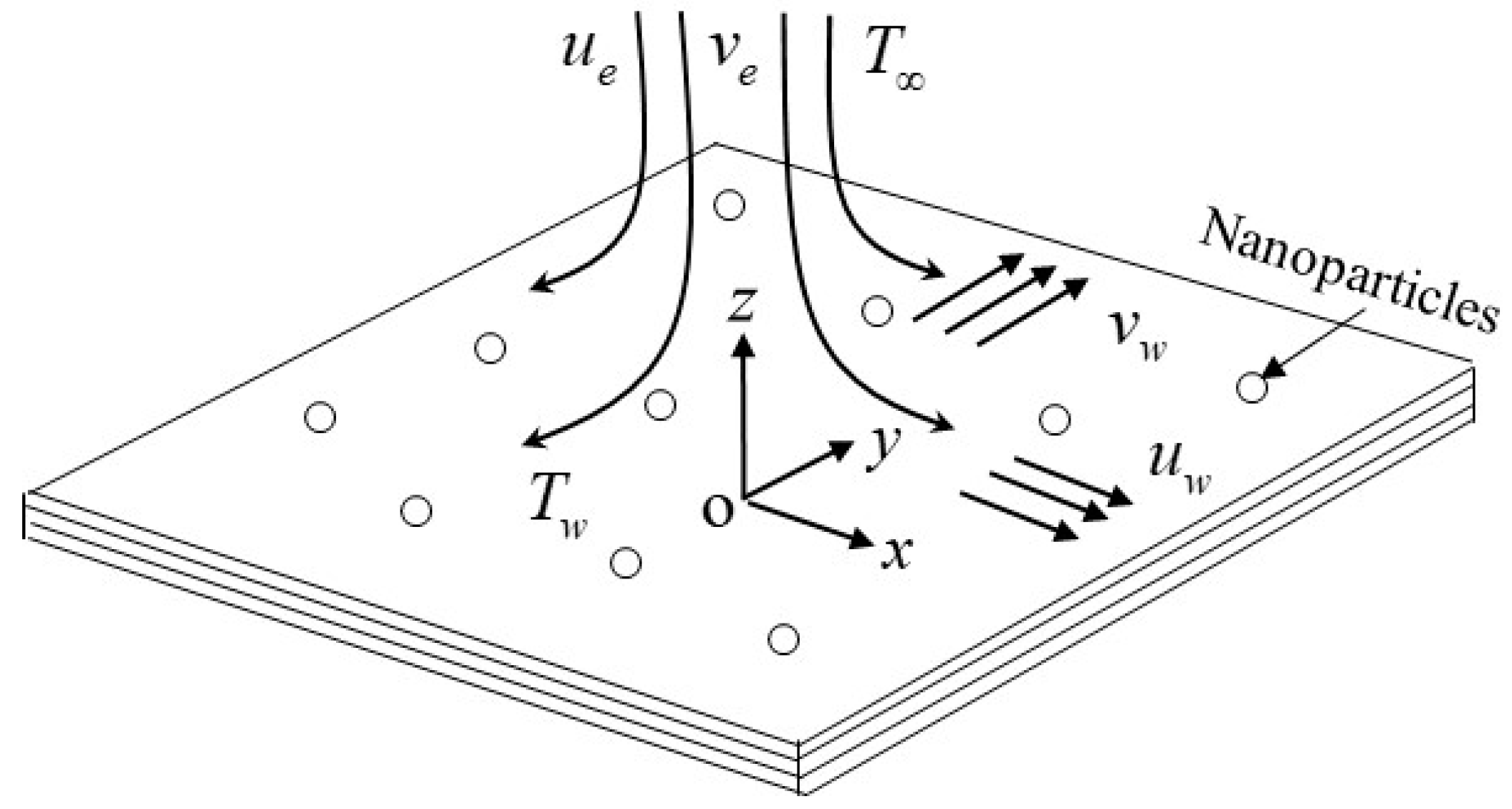
2. Mathematical Model

Consider the unsteady three-dimensional MHD non-axisymmetric Homann stagnation point flow of a hybrid Al₂O₃-Cu/water nanofluid with a stretching/shrinking sheet on the $x,y-$ plane where $x,y$ and $z$ are Cartesian coordinates with the $z-$ axis measured in the horizontal direction and the axes $x$ and $y$ are in the plane $z=0$ as illustrated in Figure 1, respectively. We assume that the constant surface temperature $T_w$ is stretched and shrunk in the $x$ and $y$ directions by the velocities $u_w=\frac{\epsilon cx}{1+\alpha t}$ and $v_w=\frac{\epsilon cy}{1+\alpha t}$ The uniform temperature is given by $T_{\infty }$ and $B_0$ is introduced to the stretching/shrinking sheet in an orthogonal direction as a transverse uniform magnetic field. Meanwhile, the modified non-asymmetrically free streamflow along the $x,y$ and $z$ axes is described by ([9]):

$$u_e\left(x\right)=\left(a+b\right)x,v_e\left(y\right)=\left(a-b\right)y,w_e\left(z\right)=-2az.$$

(1)

Here, $a$ is the strain rate and $b$ is the shear rate of stagnation point flow, correspondingly. By adapting the Tiwari and Das [30] nanofluid model, the continuity, momentum, and the energy equations of the hybrid nanofluid can be written as follows:

$$\frac{\partial u}{\partial x}+\frac{\partial v}{\partial y}+\frac{\partial w}{\partial z}=0,$$

(2)

$$\frac{\partial u}{\partial t}+u\frac{\partial u}{\partial x}+v\frac{\partial u}{\partial y}+w\frac{\partial u}{\partial z}=\frac{\partial u_e}{\partial t}+u_e\frac{\partial u_e}{dx}+\frac{{\mu }_{hnf}}{{\rho }_{hnf}}\frac{{\partial }^{2}u}{\partial z^2}-\frac{{\sigma }_{hnf}}{{\rho }_{hnf}}{B}^2\left(u-u_e\right),$$

(3)

$$\frac{\partial v}{\partial t}+u\frac{\partial v}{\partial x}+v\frac{\partial v}{\partial y}+w\frac{\partial v}{\partial z}=\frac{\partial v_e}{\partial t}+v_e\frac{\partial v_e}{dx}+\frac{{\mu }_{hnf}}{{\rho }_{hnf}}\frac{{\partial }^{2}v}{\partial z^2}-\frac{{\sigma }_{hnf}}{{\rho }_{hnf}}{B}^2\left(v-v_e\right),$$

(4)

$$\frac{\partial T}{\partial t}+u\frac{\partial T}{\partial x}+v\frac{\partial T}{\partial y}+w\frac{\partial T}{\partial z}=\frac{k_{hnf}}{{(\rho C_p)}_{hnf}}\frac{{\partial }^{2}T}{\partial z^2}.$$

(5)

The velocity component in $x-$ direction is given by $u$, while v is in $y-$ direction. Next, the boundary conditions are:

$$\begin{array}{l}t<0:u=v=w=0\mathrm{for}\mathrm{any}x,y,z,\\ t\ge 0:u=u_w,v=v_w,w=0,T=T_w\mathrm{at}z=0,\\ u\to u_e=\frac{\left(a+b\right)x}{1+\alpha t},v\to v_e=\frac{\left(a-b\right)x}{1+\alpha t},w_e\to \frac{-2az}{1+\alpha t},T\to T_{\infty }\mathrm{as}z\to \infty .\end{array}$$

(6)

Note that $T$ is the hybrid nanofluid temperature, ${\mu }_{hnf}$ is the dynamic viscosity of the hybrid nanofluid, ${\rho }_{hnf}$ is the density of the hybrid nanofluid, $k_{hnf}$ is the thermal conductivity of the hybrid nanofluid, ${(\rho C_p)}_{hnf}$ is the heat capacity of the hybrid nanofluid, ${\sigma }_{hnf}$ is the electrical conductivity of the hybrid nanofluid, and the time-dependent of a transverse magnetic field is given by $B^2=B_0^2/\left(1+\alpha t\right)$ in detail.

The hybrid nanofluids thermophysical properties are specified in

Table 1. Thermophysical properties of hybrid nanofluids (Devi and Devi [41,51]).

Properties	Hybrid Nanofluid
Density	${\rho }_{hnf}=(1-{\varphi }_2)[(1-{\varphi }_1){\rho }_f+{\varphi }_1{\rho }_{s1}]+{\varphi }_2{\rho }_{s2}$
Heat capacity	${\left(\rho C_p\right)}_{hnf}=\left(1-{\varphi }_2\right)\left[\left(1-{\varphi }_1\right){\left(\rho C_p\right)}_f+{\varphi }_1{\left(\rho C_p\right)}_{s1}\right]+{\varphi }_2{\left(\rho C_p\right)}_{s2}$
Dynamic viscosity	${\mu }_{hnf}=\frac{{\mu }_f}{{(1-{\varphi }_1)}^{2.5}{(1-{\varphi }_2)}^{2.5}}$
Thermal conductivity	$\frac{k_{hnf}}{k_{nf}}=\frac{k_{s2}+2k_{nf}-2{\varphi }_2(k_{nf}-k_{s2})}{k_{s2}+2k_{nf}+{\varphi }_2(k_{nf}-k_{s2})},$ where, $\frac{k_{nf}}{k_f}=\frac{k_{s1}+2k_f-2{\varphi }_1(k_f-k_{s1})}{k_{s1}+2k_f+{\varphi }_1(k_f-k_{s1})}$

, as demonstrated by Devi and Devi [41,51]. At this point, $\varphi$ is the volume fraction of nanoparticles, ${\rho }_f$ and ${\rho }_s$ are the base fluid density and hybrid nanoparticles, $C_p$ is the heat capacity, ${(\rho C_p)}_f$ and ${(\rho C_p)}_s$ represent capacitance heating of the base fluid and hybrid nanoparticles, and finally $k_f$ and $k_s$ are the thermal conductivities of the base fluid and hybrid nanoparticles, respectively. Meanwhile, the thermophysical properties of the fluid and nanoparticles for aluminum oxide, copper, and the base fluid (water) are given in

Table 2. Thermophysical properties of nanoparticles and base fluid (Oztop and Abu-Nada [52]).

Properties	Al2O3	Cu	H2O
$\rho ({\mathrm{kg}/\mathrm{m}}^3)$	3970	8933	997.1
$C_p(\mathrm{J}/\mathrm{kgK})$	765	385	4179
$k(\mathrm{W}/\mathrm{mK})$	40	400	0.613
$\beta \times {10}^{-5}(\mathrm{mK})$	0.85	1.67	21

.

Now, pursuing Mahapatra and Sidui [10], the resulting similarity transformation is proposed to achieve the similarity solutions:

$$\begin{array}{l}u=\frac{cx{f}^{\prime }\left(\eta \right)}{1+\alpha t},v=\frac{cy{g}^{\prime }\left(\eta \right)}{1+\alpha t},w=-\sqrt{\frac{\nu c}{1+\alpha t}}\left(f+g\right),\theta \left(\eta \right)=\frac{\left(T-T_{\infty }\right)}{\left(T_w-T_{\infty }\right)},\\ \eta =\sqrt{\frac{c}{\nu \left(1+\alpha t\right)}}z,\end{array}$$

(7)

where the prime denotes differentiation with respect to $\eta$. By substituting (7) into the steady-state Equations (2)–(5), the following ordinary differential equations are obtained:

$$\begin{array}{l}\frac{{\mu }_{hnf}/{\mu }_f}{{\rho }_{hnf}/{\rho }_f}{f}^{‴}+A\left(\frac{1}{2}\eta +f+g\right)f^{″}+A{f}^{\prime }-{f^{\prime }}^2-A\left(\lambda +\gamma \right)+{\left(\lambda +\gamma \right)}^2\\ -M\left(f^{\prime }-\lambda -\gamma \right)=0,\end{array}$$

(8)

$$\begin{array}{l}\frac{{\mu }_{hnf}/{\mu }_f}{{\rho }_{hnf}/{\rho }_f}{g}^{‴}+A\left(\frac{1}{2}\eta +f+g\right)g^{″}+A{g}^{\prime }-{g^{\prime }}^2-A\left(\lambda -\gamma \right)+{\left(\lambda -\gamma \right)}^2\\ -M\left(g^{\prime }-\lambda +\gamma \right)=0,\end{array}$$

(9)

$$\frac{1}{\mathrm{Pr}}\frac{k_{hnf}/k_f}{\rho C_p{}_{hnf}/\rho C_p{}_f}{\theta }^{″}+\left(A\frac{1}{2}\eta +f+g\right){\theta }^{\prime }=0,$$

(10)

with the boundary conditions (6) which are converted to:

$$\begin{array}{l}f(0)=g(0)=0,f^{\prime }(0)=g^{\prime }(0)=\epsilon ,\theta (0)=1,\\ f^{\prime }(\eta )\to \lambda +\gamma ,g^{\prime }(\eta )\to \lambda -\gamma ,\theta (\eta )\to 0,\mathrm{as}\eta \to \infty .\end{array}$$

(11)

In the equations mentioned above, $A=\alpha /c$ represents the unsteadiness parameter, $\lambda =a/c$ is a ratio of the surrounding fluid strain rate to the surface strain rate, $\gamma =b/c$ is the surrounding fluid shear rate ratio to the strain rate of the sheet, $M=\frac{{\sigma }_{hnf}/{\sigma }_f}{{\rho }_{hnf}/{\rho }_f}\frac{B_0^2}{c}$ denotes the magnetic parameter and $\mathrm{Pr}={\nu }_f/{\alpha }_f$ indicates the Prandtl number. The parameter of stretching/shrinking is meant by $\epsilon$ where $\epsilon >0$ determines the stretching sheet, while $\epsilon <0$ reflects the shrinking sheet. The related quantities of interest in this study are the skin friction coefficient, $C_{fx}$ and $C_{fy}$ along the $x-$ and $y-$ directions and the local Nusselt number $N{u}_x$, which is specified as

$$C_{fx}=\frac{{\tau }_{wx}}{{\rho }_f{u}_e{}^2},C_{fy}=\frac{{\tau }_{wy}}{{\rho }_f{v}_e{}^2},N{u}_x=\frac{x{q}_w}{k_f\left(T_w-T_{\infty }\right)},$$

(12)

where ${\tau }_{wx}$, ${\tau }_{wy}$ are the shear stresses along the $x-,y-$ axes and $q_w$ represents the heat flux, correspondingly. Such terms can be defined by

$${\tau }_{wx}={\mu }_{hnf}{\left(\frac{\partial u}{\partial z}\right)}_{z=0},{\tau }_{wy}={\mu }_{hnf}{\left(\frac{\partial v}{\partial z}\right)}_{z=0},q_w=-k_{hnf}{\left(\frac{\partial T}{\partial z}\right)}_{z=0}.$$

(13)

By prompting Equations (7), (12) and (13), we get:

$$\begin{array}{l}{\left(\lambda +\gamma \right)}^{3/2}{\mathrm{Re}}_x^{1/2}{C}_{f_x}=\frac{{\mu }_{hnf}}{{\mu }_f}{f}^{″}\left(0\right),{\left(\lambda -\gamma \right)}^{3/2}{\mathrm{Re}}_y^{1/2}{C}_{f_y}=\frac{{\mu }_{hnf}}{{\mu }_f}{g}^{″}\left(0\right),\\ {\left(\lambda +\gamma \right)}^{1/2}{\mathrm{Re}}_x{}^{-1/2}N{u}_x=-\frac{k_{hnf}}{k_f}{\theta }^{\prime }(0),\end{array}$$

(14)

where ${\mathrm{Re}}_x=\frac{(a+b)x^2}{\left(1+\alpha t\right){\nu }_f}$ and ${\mathrm{Re}}_y=\frac{(a+b)y^2}{\left(1+\alpha t\right){\nu }_f}$ are the local Reynolds number along the $x-$ and $y-$ directions, respectively.

3. Stability Analysis

The system of Equations (8)$–$(10) along with the boundary conditions (11), is capable of generating more than one solution and ultimately permits the requirement analysis of the flow to identify the reliable and feasible solution. Going through the outstanding work done by Merkin [53] and Merrill et al. [54] in the stability analysis, the application of an unstable form of the boundary layer problem is analyzed by using the time variable and a dimensionless time variable denoted by $\tau$ [55]. Next, we consider the following new similarity variables:

$$\begin{array}{l}u=\frac{cx}{1+\alpha t}\frac{\partial f}{\partial \eta }\left(\eta ,\tau \right),v=\frac{cy}{1+\alpha t}\frac{\partial g}{\partial \eta }\left(\eta ,\tau \right),w=-\sqrt{\frac{\nu c}{1+\alpha t}}\left[f\left(\eta ,\tau \right)+g\left(\eta ,\tau \right)\right],\\ \theta \left(\eta \right)=\frac{\left(T-T_{\infty }\right)}{\left(T_w-T_{\infty }\right)},\eta =\sqrt{\frac{c}{\nu \left(1+\alpha t\right)}}z,\tau =\frac{ct}{1+\alpha t}.\end{array}$$

(15)

Using the similarity variables of Equation (15) into Equations (8)$–$(10), the altered differential equations and the boundary conditions are as follows:

$$\begin{array}{l}\frac{{\mu }_{hnf}/{\mu }_f}{{\rho }_{hnf}/{\rho }_f}\frac{{\partial }^{3}f}{\partial {\eta }^3}+\left(A\frac{1}{2}\eta +f+g\right)\frac{{\partial }^{2}f}{\partial {\eta }^2}+A\frac{\partial f}{\partial \eta }-{\left(\frac{\partial f}{\partial \eta }\right)}^2-A\left(\lambda +\gamma \right)+{\left(\lambda +\gamma \right)}^2\\ -M\left(\frac{\partial f}{\partial \eta }-\lambda -\gamma \right)-\left(1-A\tau \right)\frac{{\partial }^{2}f}{\partial \eta \partial \tau }=0,\end{array}$$

(16)

$$\begin{array}{l}\frac{{\mu }_{hnf}/{\mu }_f}{{\rho }_{hnf}/{\rho }_f}\frac{{\partial }^{3}g}{\partial {\eta }^3}+\left(A\frac{1}{2}\eta +f+g\right)\frac{{\partial }^{2}g}{\partial {\eta }^2}+A\frac{\partial g}{\partial \eta }-{\left(\frac{\partial g}{\partial \eta }\right)}^2-A\left(\lambda -\gamma \right)+{\left(\lambda -\gamma \right)}^2\\ -M\left(\frac{\partial g}{\partial \eta }-\lambda +\gamma \right)-\left(1-A\tau \right)\frac{{\partial }^{2}g}{\partial \eta \partial \tau }=0,\end{array}$$

(17)

$$\frac{1}{\mathrm{Pr}}\frac{k_{hnf}/k_f}{\rho C_p{}_{hnf}/\rho C_p{}_f}\frac{{\partial }^2\theta }{\partial {\eta }^2}+\left(A\left(\frac{1}{2}\eta -\tau \right)+f+g+1\right)\frac{\partial \theta }{\partial \eta }-\left(1-A\tau \right)\frac{\partial \theta }{\partial \tau }=0,$$

(18)

$$\begin{array}{l}f(0,\tau )=g(0,\tau )=0,\frac{\partial f}{\partial \eta }(0,\tau )=\frac{\partial g}{\partial \eta }(0,\tau )=\epsilon ,\theta (0,\tau )=1,\\ \frac{\partial f}{\partial \eta }(\eta ,\tau )\to \lambda +\gamma ,\frac{\partial g}{\partial \eta }(\eta ,\tau )\to \lambda -\gamma ,\theta (\eta ,\tau )\to 0,\mathrm{as}\eta \to \infty .\end{array}$$

(19)

Weidman et al. [55] highlighted that the stability of solutions is introduced by determining the system’s decay or initial growth. This can be achieved via considering the following perturbation expressions of the primary flow $f=f_0(\eta ),g=g_0(\eta )$ and $\theta ={\theta }_0(\eta )$ with the resulting equation:

$$\begin{array}{l}f\left(\eta ,\tau \right)=f_0\left(\eta \right)+e^{-\omega \tau }F\left(\eta \right),g\left(\eta ,\tau \right)=g_0\left(\eta \right)+e^{-\omega \tau }G\left(\eta \right),\\ \theta \left(\eta ,\tau \right)={\theta }_0\left(\eta \right)+e^{-\omega \tau }H\left(\eta \right),\end{array}$$

(20)

where $\omega$ is an unknown parameter of the eigenvalue, $F(\eta ),G(\eta )$ and $H(\eta )$ are comparatively slight to $f_0(\eta ),g_0(\eta )$ and ${\theta }_0(\eta )$. Substituting (20) into Equations (16)$–$(18) we attained the following system of equations:

$$\begin{array}{l}\frac{{\mu }_{hnf}/{\mu }_f}{{\rho }_{hnf}/{\rho }_f}\frac{{\partial }^{3}F}{\partial {\eta }^3}+\left(A\frac{1}{2}\eta +f_0+g_0\right)\frac{{\partial }^{2}F}{\partial {\eta }^2}+\left(A-M+\left(1-A\tau \right)\omega -2\frac{\partial f_0}{\partial \eta }\right)\frac{\partial F}{\partial \eta }\\ +\left(F+G\right)\frac{{\partial }^2{f}_0}{\partial {\eta }^2}=0,\end{array}$$

(21)

$$\begin{array}{l}\frac{{\mu }_{hnf}/{\mu }_f}{{\rho }_{hnf}/{\rho }_f}\frac{{\partial }^{3}G}{\partial {\eta }^3}+\left(A\frac{1}{2}\eta +f_0+g_0\right)\frac{{\partial }^{2}G}{\partial {\eta }^2}+\left(A-M+\left(1-A\tau \right)\omega -2\frac{\partial g_0}{\partial \eta }\right)\frac{\partial G}{\partial \eta }\\ +\left(F+G\right)\frac{{\partial }^2{g}_0}{\partial {\eta }^2}=0,\end{array}$$

(22)

$$\frac{1}{\mathrm{Pr}}\frac{k_{hnf}/k_f}{{(\rho C_p)}_{hnf}/{(\rho C_p)}_f}\frac{{\partial }^{2}H}{\partial {\eta }^2}+(F+G)\frac{\partial {\theta }_0}{\partial \eta }+\left(A\frac{1}{2}\eta +f_0+g_0\right)\frac{\partial H}{\partial \eta }+\omega H=0,$$

(23)

subject to the boundary conditions:

$$\begin{array}{l}F(0)=G(0)=0,\frac{\partial F}{\partial \eta }(0)=\frac{\partial G}{\partial \eta }(0)=0,H(0)=0,\\ \frac{\partial F}{\partial \eta }(\infty )\to 0,\frac{\partial G}{\partial \eta }(\infty )\to 0,H(\infty )\to 0.\end{array}$$

(24)

The stability of the steady-state flow and heat transfer solutions $f_0(\eta ),g_0(\eta )$ and ${\theta }_0(\eta )$ was implemented by setting $\tau =0$ with $F=f_0(\eta ),G=g_0(\eta )$ and $H={\theta }_0(\eta )$ in (21)$–$(24). Finally, the initial development or the solution decay of the solution (20) is identified. The value of $\omega$ is obtained by solving the following eigenvalue problem:

$$\frac{{\mu }_{hnf}/{\mu }_f}{{\rho }_{hnf}/{\rho }_f}{F}_0^{‴}+\left(A\frac{1}{2}\eta +f_0+g_0\right)F_0^{″}+\left(A-M+\omega -2f_0^{\prime }\right)F^{\prime }+\left(F+G\right)f_0^{″}=0,$$

(25)

$$\frac{{\mu }_{hnf}/{\mu }_f}{{\rho }_{hnf}/{\rho }_f}{G}_0^{‴}+\left(A\frac{1}{2}\eta +f_0+g_0\right)G_0^{″}+\left(A-M+\omega -2g_0^{\prime }\right)G^{\prime }+\left(F+G\right)g_0^{″}=0,$$

(26)

$$\frac{1}{\mathrm{Pr}}\frac{k_{hnf}/k_f}{{(\rho C_p)}_{hnf}/{(\rho C_p)}_f}{H}^{″}+(F+G){\theta }_0{}^{\prime }+\left(A\frac{1}{2}\eta +f_0+g_0\right)H^{\prime }+\omega H=0,$$

(27)

along with the conditions:

$$\begin{array}{l}{F}_0(0)=G_0(0)=0,F_0^{\prime }(0)=G_0^{\prime }(0)=0,H_0(0)=0,\\ F_0^{\prime }(\infty )\to 0,G_0^{\prime }(\infty )\to 0,H_0(\infty )\to 0.\end{array}$$

(28)

The range of possible eigenvalues can be determined by relaxing a boundary condition on $F_0^{\prime }(\eta )$ according to the previous research by Harris et al. [56]. In this study, the condition $F_0^{\prime }(\infty )\to 0$ is relaxed, and the linear eigenvalue problem (25)$–$(28) is solved together with the new boundary condition $F_0^{″}(0)=1$ for a fixed value of ${\omega }_1.$ The flow is considered unstable if the smallest eigenvalue ${\omega }_1.$ is negative, which indicates an initial growth of disturbances occurred, while a positive value of the smallest eigenvalue signifies that the flow is physically achievable and stable.

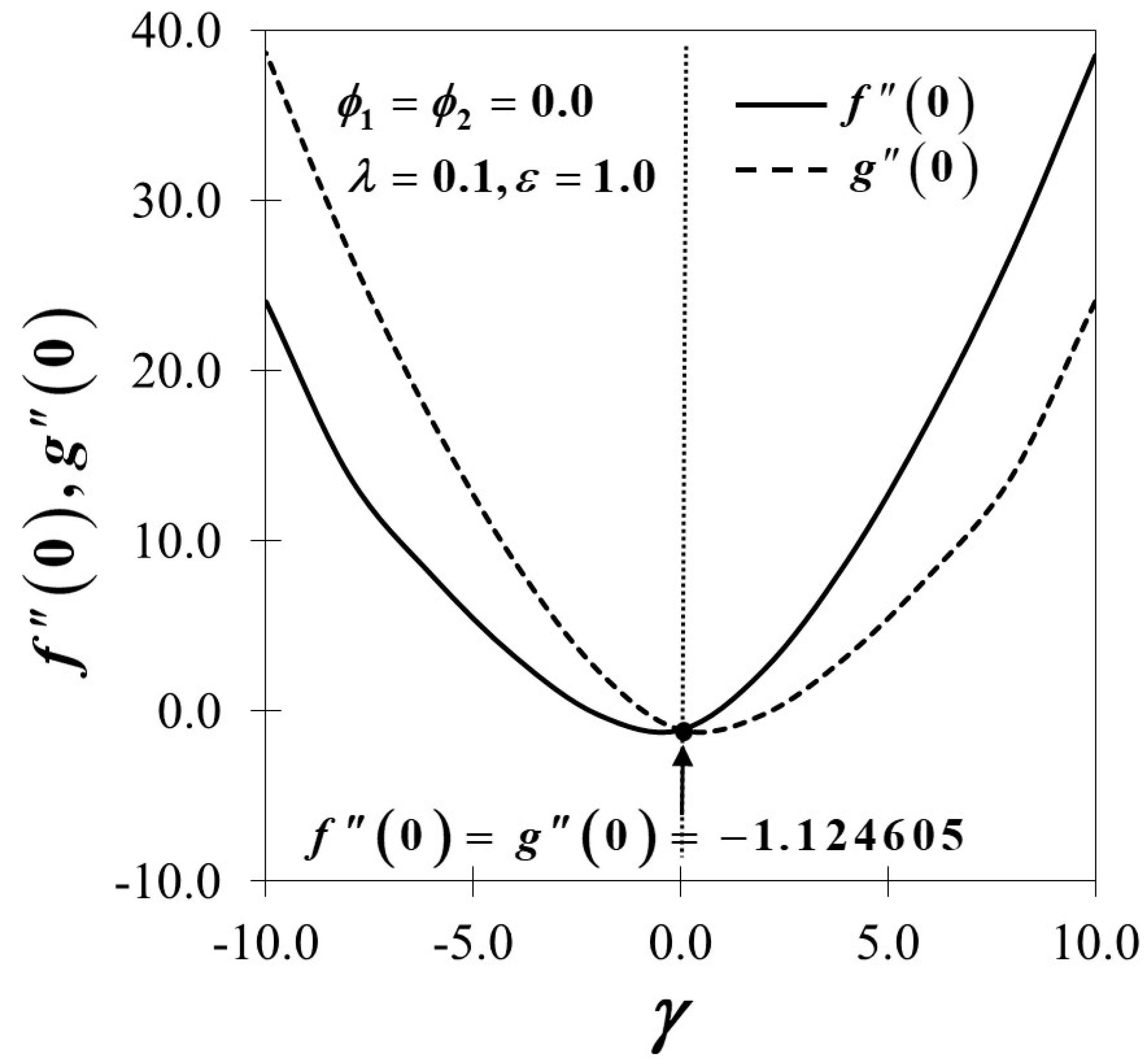
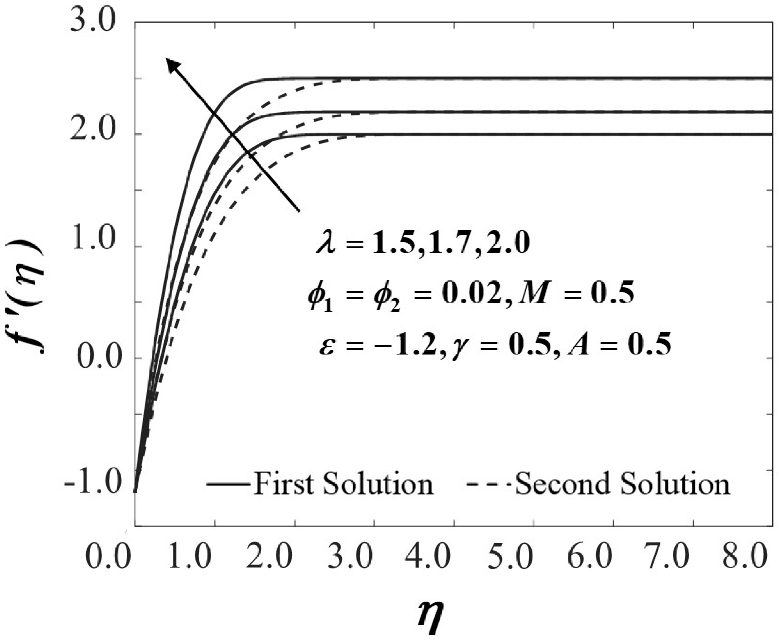
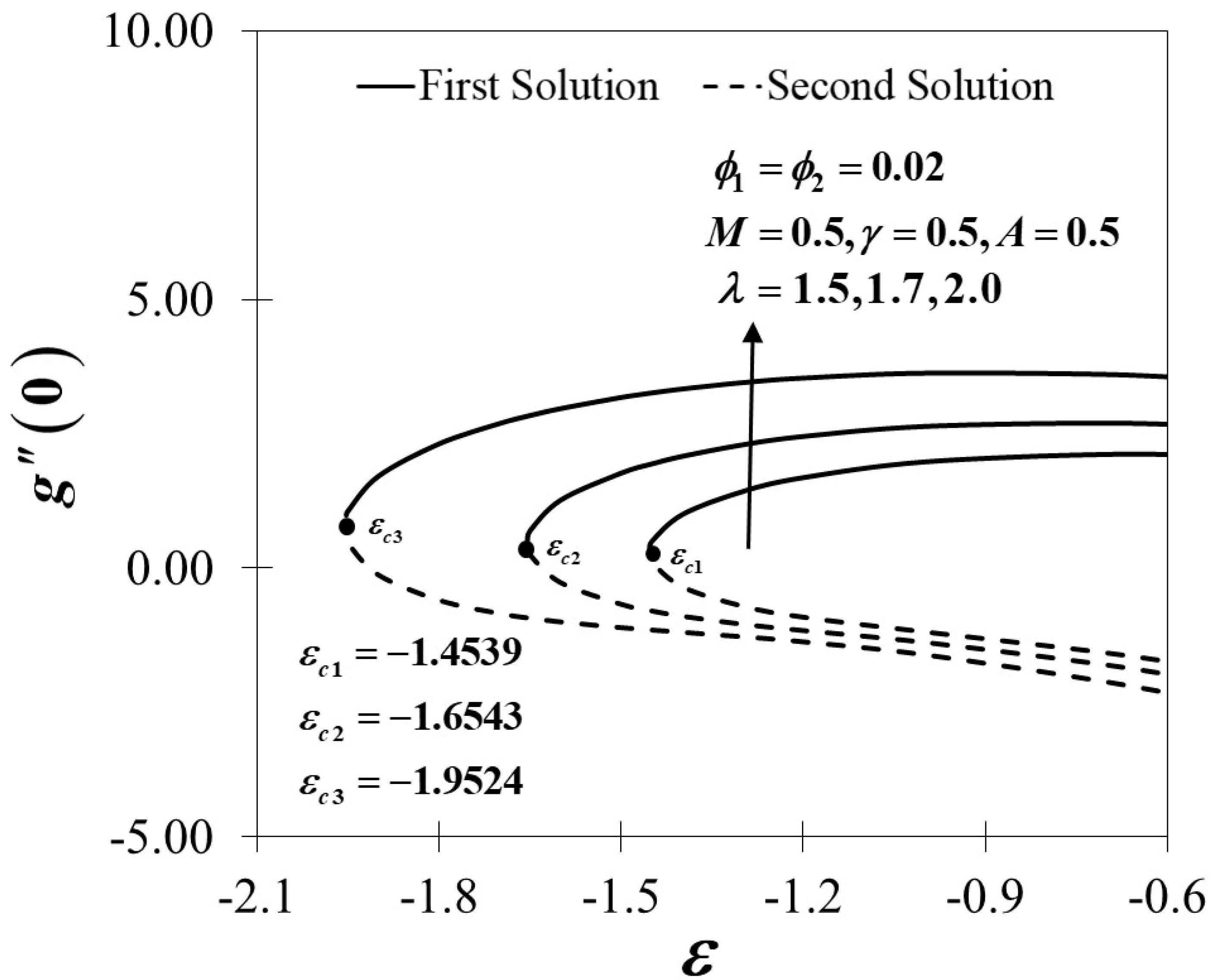
4. Results and Discussion

The bvp4c function in Matlab is adopted to produce the results of the nonlinear system of ordinary differential Equations (8)$–$(10) together with the boundary conditions (11). The relative error tolerance is set as ${10}^{-10}$ to gain the results of the numerical outcomes and stability analysis.

Table 3. Computational time to generate the values of $f^{″}(0)$ as $\lambda$ varies when ${\varphi }_1={\varphi }_2=0,\gamma =0,\epsilon =1,M=0,\mathrm{A}=0,$ and $\mathrm{Pr}=6.2$.

$\mathit{\lambda }$	${\mathit{f}}^{″}(0)$	$\mathbf{Time},\mathit{t}(\mathbf{s})$
$0.1$	$-1.12460540$	$0.851$
$0.2$	$-1.05562203$	$0.960$
$0.5$	$-0.75344581$	$0.877$
$1.0$	$0$	$1.474$
$2.0$	$2.20708771$	$1.419$

presents that the average central processing unit (CPU) time required for computing each result in

Table 4. Results of $f^{″}(0)$ for specific values of $\lambda$ when ${\varphi }_1=0.0,{\varphi }_2=0.0,\gamma =0,\epsilon =1,M=0,$ $\mathrm{A}=0,$ and $\mathrm{Pr}=6.2$.

λ	Present Result	Mahapatra and Sidui [10]	${\mathit{\epsilon }}_{\mathit{r}}=\left|\frac{\mathit{r}-\mathit{s}}{\mathit{s}}\right|\times 100\mathit{\%}$	Nawaz and Hayat [57]	${\mathit{\epsilon }}_{\mathit{r}}=\left|\frac{\mathit{r}-\mathit{s}}{\mathit{s}}\right|\times 100\mathit{\%}$
$0.1$	$-1.12460540$	$-1.124000$	$0.053832\%$	$-1.124600$	$0.000480\%$
$0.2$	$-1.05562203$	$-1.054400$	$0.115764\%$	$-1.055610$	$0.001139\%$
$0.5$	$-0.75344581$	$-0.753400$	$0.006080\%$	$-0.753100$	$0.045897\%$
$1.0$	$0.00000000$	$0.000000$	$0.000000\%$	$0.000000$	$0.000000\%$
$2.0$	$2.20708771$	$2.190200$	$0.765158\%$	$-$	$-$

$\ast {\epsilon }_r$ is the estimate percentage relative error between the present result, $r$ and previous result, $s$.

is approximately 1.4 s, and the dual solutions were obtained by indicating different initial guesses which must satisfy the far-field boundary conditions (11) asymptotically. The numerical results are validated with the numerical results produced by Mahapatra and Sidui [10] and Nawaz and Hayat [57] by collating the values of the shear stress $f^{″}(0)$ of an axisymmetric $(\gamma =0)$ stagnation point flow of a viscous fluid with the exclusion of magnetic field and the unsteady parameter, which is depicted in Table 4. It demonstrates excellent agreement with the previous literature; hence, the practicality and effectiveness of the bvp4c method are verified. The estimated relative error, ${\epsilon }_r$ is also measured, and it shows that the calculated values of ${\epsilon }_r$ are relatively small between the present and previous results. Figure 2 exhibits the variation of the wall shear stress parameter $f^{″}(0)$ and $g^{″}(0)$ towards the difference value of $\gamma$ when ${\varphi }_1={\varphi }_2=M=A=0,\lambda =0.1,\epsilon =1.0$ and $\mathrm{Pr}=1.0$ where the dotted lines correspond to the asymptotic behaviour of $f^{″}(0)$ and $g^{″}(0)$ which is in excellent agreement with Mahapatra and Sidui [10] who pursued a standard fourth-order Runge-Kutta integration technique in their study. This justifies the role of the bvp4c numerical technique as a dependable practice, and the present results are valid and correct.

The dimensionless velocity profiles $f^{\prime }(\eta )$ and $g^{\prime }(\eta )$ for different values of $\lambda$ are illustrated in Figure 3 and Figure 4. The figures prove that the profiles of the velocity comply with the far-field boundary conditions of Equation (11) asymptotically. The maximum value of the velocity gradient with the lowest thickness of the momentum boundary layer is preserved for the largest value of $\lambda$. Notably, the distance of two adjacent profiles increases remarkably with the increased amount of $\lambda$ in both the first and second solutions. Figure 5 and Figure 6 portray the variations of $f^{″}(0)$ and $g^{″}(0)$ towards $\epsilon$ for different values of $\lambda$ in hybrid nanofluids with the existence of the magnetic field and the influences of the unsteadiness parameter. An enrichment in the amounts of $\lambda$ embarking on the augmentation of both $\lambda +\gamma$ and $\lambda -\gamma$ provide a significant effect to the surface shear stresses. The variations of $f^{″}(0)$ are expected to be higher by the increasing value of $\lambda +\gamma$ yet decrease when $\lambda +\gamma$ is decreased, and the same trend is expected in $g^{″}(0)$ with $\lambda -\gamma$. On the other hand, the effect of the nanoparticles volume fraction is observed in Figure 7, Figure 8 and Figure 9, respectively. Surprisingly, the critical values of the various usage of the nanoparticles’ volume fraction give no significant effect to the trend of the nanofluid $({\varphi }_1=0.02,{\varphi }_2=0.00)$ and hybrid nanofluid flow $({\varphi }_1=0.02,{\varphi }_2=0.002,0.04).$ It is observed that the reduced skin friction coefficient in $x$ and $y$ directions, as presented in Figure 7 and Figure 8, and the reduced local Nusselt number in Figure 9 upsurges with the rising in the nanoparticles’ volume fraction. This is due to the fact that more kinetic energy is produced with a higher concentration of nanoparticles and thus, enhances the heat transfer of the fluid particles. This finding also corresponds with several present particle-laden direct numerical studies (DNS), which reveal that the roughness components appear to redistribute the energy and, therefore, decrease the overall large-scale near-wall anisotropy of the flow pattern (see Yuan and Piomelli [58] and Ghodke and Apte [59]).

Figure 10, Figure 11 and Figure 12 exhibit the influence of the magnetic parameter on $f^{″}(0)$, $g^{″}(0)$ and $-{\theta }^{\prime }(0)$ which shows a prominent effect on the fluid flow of the shrinking sheet. The reduced skin friction coefficient in both the $x-$ and $y-$ directions rise and eventually increase the value of $-{\theta }^{\prime }(0)$ with the escalation of $M$ due to the occurrence of the Lorentz force, which acts to retard the fluid flow. The Lorentz force creates resistance to the motion of the fluid particles and then consequently reduces the fluid velocity. The synchronism of the magnetic and electric field that occurred from the formation of the Lorentz force tends to slow down the fluid movement. The boundary layer becomes thinner in both directions as proven in Figure 13 and Figure 14 as $M$ increases due to the delayed flow, hence contributing to the increment of $f^{″}(0)$ and $g^{″}(0).$ On the other hand, Figure 15 advertises the variations of the non-dimensional temperature profiles for different values of $M$ which tend to decrease in the first solution but show a reverse trend in the second solution. The figures clearly reveal that the thicknesses of the thermal boundary layers decrease with the increase of $M$ Practically, by restricting the magnetic field intensity, the progression of the thermal boundary layers’ thicknesses can be managed and, thus, be able to reduce the temperature profile distributions.

The effect of the unsteadiness parameter $A$ on $f^{″}(0)$, $g^{″}(0)$ and $-{\theta }^{\prime }(0)$ is depicted in Figure 16, Figure 17 and Figure 18, respectively. Increasing the values of $A$ results in a reduction of the skin friction coefficients in both directions, as illustrated in Figure 16 and Figure 17, which consequently decreases the reduced local Nusselt number. The fact that the unsteadiness parameter affects the velocity and temperature profile is proven in Figure 19, Figure 20 and Figure 21. The velocity of the fluid is in decline along the surface of the sheet due to the increasing value of the shear stress and subsequently shrinks the thickness of the momentum boundary layer nearby the wall, as displayed in Figure 19 and Figure 20, accordingly. The increasing value of $A$ decreases in the temperature profile of the hybrid nanofluid, as shown in Figure 21, which is understandable because the spaces between the molecules become higher in unsteady flow and proportionately decrease the temperature profile and improve the cooling rates of the fluid. Therefore, the unsteadiness parameter should be highlighted and well considered for practical purposes.

Since the dual solutions noticeably exist, as illustrated in Figure 3, Figure 4, Figure 5, Figure 6, Figure 7, Figure 8, Figure 9, Figure 10, Figure 11, Figure 12, Figure 13, Figure 14, Figure 15, Figure 16, Figure 17, Figure 18, Figure 19, Figure 20 and Figure 21, a stability analysis is performed to discover a significant solution between the first and second solutions. This process is achievable by clarifying the eigenvalue problems in Equations (25)$–$(27) using bvp4c in Matlab, which produce an infinite set of ${\omega }_1<{\omega }_2<{\omega }_3\dots \dots$. The stability of the flow is reliant on the smallest positive eigenvalue ${\omega }_1$ since there exists an initial decay of disturbances. In contrast, there is an initial growth of perturbations if the smallest eigenvalue ${\omega }_1$ is negative, which signifies that the solution is unstable. As depicted in

Table 5. Smallest eigenvalues ${\omega }_1$ when ${\varphi }_1={\varphi }_2=0.02,\lambda =1.5,\gamma =0.5,M=0.5,\mathrm{A}=0.5\mathrm{and}\mathrm{P}r=6.2$.

$\mathit{\epsilon }$	$\mathbf{First}\mathbf{Solution},{\mathit{\omega }}_1$	$\mathbf{Second}\mathbf{Solution},{\mathit{\omega }}_1$
$-$1.4	0.9181	$-$0.3952
$-$1.452	0.1712	$-$0.1469
$-$1.4532	0.1158	$-$0.0979
$-$1.4534	0.1040	$-$0.0869
$-$1.4536	0.0902	$-$0.0744
$-$1.4538	0.0741	$-$0.0593
$-$1.45388	0.0665	$-$0.0521

, the lowest eigenvalues for the first solution are positive, while the second solution is negative. In conclusion, the first solution is stable and physically reliable, while the second solution is unstable and unreal.

5. Conclusions

The current analysis is devoted to examining the unsteady three-dimensional non-axisymmetric Homann stagnation point flow of alumina (Al₂O₃) and copper (Cu) hybrid nanofluids in the presence of MHD. The governing partial differential equations are transformed into a system of ordinary differential equations by using a similarity transformation and appropriately solved by a bvp4c function in Matlab. An increment in $\lambda$ may upsurge the velocity gradient and thus decline the momentum boundary layer thickness. A high concentration of the nanoparticle volume fraction speeds up the molecules’ kinetic energy and then enhances the heat transfer process of the fluid particles. The increment in the intensity of the magnetic parameter $M$ increases the local Nusselt number and the skin friction coefficient. Further, the increasing value of $A$ decreases the hybrid nanofluid temperature and eventually improves the cooling rates of the fluid. Dual solutions were disclosed in this study, and the analysis of solution stability confirmed that the first solutions are stable and physically reliable.

References

1. Fisher, E. Extrusion of Plastics; Wiley: New York, NY, USA, 1976. [Google Scholar]
2. Rauwendaal, C. Polymer Extrusion; Hanser Publication: Munich, Germany, 1985. [Google Scholar]
3. Ibrahim, W.; Shankar, B.; Nandeppanavar, M.M. MHD stagnation point flow and heat transfer due to nanofluid towards a stretching sheet. Int. J. Heat Mass Transf. 2013, 56, 1–9. [Google Scholar] [CrossRef]
4. Hiemenz, K. Die Grenzschicht an einem in den gleichfÖrmingen Flüssigkeitsstrom eingetauchten geraden Kreiszylinder. Dinglers Polytech J. 1911, 326, 321–324. [Google Scholar]
5. Homann, F. Der Einfluss grosser Zähigkeit bei der Strömung um den Zylinder und um die Kugel. Z. Angew. Math. Mech. 1936, 16, 153–164. [Google Scholar] [CrossRef]
6. Howarth, L. CXLIV. The boundary layer in three-dimensional flow—Part II. The flow near a stagnation point. Lond. Edinb. Dublin Philos. Mag. J. Sci. 1951, 42, 1433–1440. [Google Scholar] [CrossRef]
7. Davey, A. Boundary-layer flow at a saddle point of attachment. J. Fluid Mech. 1961, 10, 593–610. [Google Scholar] [CrossRef]
8. Davey, A.; Schofield, D. Three-dimensional flow near a two-dimensional stagnation point. J. Fluid Mech. 1967, 28, 149–151. [Google Scholar] [CrossRef]
9. Weidman, P.D. Non-axisymmetric Homann stagnation-point flows. J. Fluid Mech. 2012, 702, 460–469. [Google Scholar] [CrossRef]
10. Mahapatra, T.R.; Sidui, S. Unsteady heat transfer in non-axisymmetric Homann stagnation-point flows. Z. Angew. Math. Phys. 2017, 68, 32. [Google Scholar] [CrossRef]
11. Mahapatra, T.R.; Sidui, S. Non-axisymmetric Homann stagnation-point flow of a viscoelastic fluid towards a fixed plate. Eur. J. Mech. B/Fluids 2020, 79, 38–43. [Google Scholar] [CrossRef]
12. Wang, C.Y. Stagnation flow towards a shrinking sheet. Int. J. Non. Linear Mech. 2008, 43, 377–382. [Google Scholar] [CrossRef]
13. Mahapatra, T.R.; Sidui, S. Unsteady heat transfer in non-axisymmetric Homann stagnation-point flows towards a stretching/shrinking sheet. Eur. J. Mech. B/Fluids 2019, 75, 199–208. [Google Scholar] [CrossRef]
14. Khashi’ie, N.S.; Arifin, N.M.; Pop, I.; Nazar, R.; Hafidzuddin, E.H.; Wahi, N. Non-axisymmetric Homann stagnation point flow and heat transfer past a stretching/shrinking sheet using hybrid nanofluid. Int. J. Numer. Methods Heat Fluid Flow 2020. [Google Scholar] [CrossRef]
15. Zaimi, K.; Ishak, A. Stagnation-point flow towards a stretching vertical sheet with slip effects. Mathematics 2016, 4, 27. [Google Scholar] [CrossRef]
16. Arif Ullah Khan, S.; Saleem, S.; Nadeem, A.A.A. Analysis of unsteady non-axisymmetric Homann stagnation point flow of nanofluid and possible existence of multiple solutions. Physica A 2019, 137567. [Google Scholar] [CrossRef]
17. Jusoh, R.; Nazar, R.; Pop, I. Impact of heat generation/absorption on the unsteady magnetohydrodynamic stagnation point flow and heat transfer of nanofluids. Int. J. Numer. Methods Heat Fluid Flow 2019, 30, 557–574. [Google Scholar] [CrossRef]
18. Khashi’ie, N.S.; Arifin, N.; Hafidzuddin, E.H.; Wahi, N. MHD mixed convective stagnation point flow with heat generation past a shrinking sheet. ASM Sci. J. 2019, 71–81. [Google Scholar]
19. Ali, F.M.; Naganthran, K.; Nazar, R.; Pop, I. MHD mixed convection boundary layer stagnation-point flow on a vertical surface with induced magnetic field: A stability analysis. Int. J. Numer. Methods Heat Fluid Flow 2019. [Google Scholar] [CrossRef]
20. Shehzad, S.A.; Abdullah, Z.; Alsaedi, A.; Abbasi, F.M.; Hayat, T. Thermally radiative three-dimensional flow of Jeffrey nanofluid with internal heat generation and magnetic field. J. Magn. Magn. Mater. 2016, 397, 108–114. [Google Scholar] [CrossRef]
21. Daniel, Y.S.; Aziz, Z.A.; Ismail, Z.; Salah, F. Double stratification effects on unsteady electrical MHD mixed convection flow of nanofluid with viscous dissipation and Joule heating. J. Appl. Res. Technol. 2017, 15, 464–476. [Google Scholar] [CrossRef]
22. Pavlov, K.B. Magnetohydrodynamic flow of an incompressible viscous fluid caused by deformation of a plane surface. Magn. Gidrodin. 1974, 4, 146–147. [Google Scholar]
23. Chakrabarti, A.; Gupta, A.S. Hydromagnetic flow and heat transfer over a stretching sheet. Q. Appl. Math. 1979, 37, 73–78. [Google Scholar] [CrossRef] [Green Version]
24. Vajravelu, K. Hydromagnetic flow and heat transfer over a continuous, moving, porous, flat surface. Acta Mech. 1986, 185, 179–185. [Google Scholar] [CrossRef]
25. Andersson, H.I. An exact solution of the Navier-Stokes equations for magnetohydrodynamic flow. Acta Mech. 1995, 113, 241–244. [Google Scholar] [CrossRef]
26. Lok, Y.Y.; Ishak, A.; Pop, I. MHD stagnation-point flow towards a shrinking sheet. Int. J. Numer. Methods Heat Fluid Flow 2011, 21, 61–72. [Google Scholar] [CrossRef] [Green Version]
27. Almutairi, F.; Khaled, S.M.; Ebaid, A. MHD flow of nanofluid with homogeneous-heterogeneous reactions in a porous medium under the influence of second-order velocity slip. Mathematics 2019, 7, 220. [Google Scholar] [CrossRef] [Green Version]
28. Zhu, J.; Xu, Y.; Han, X. A non-newtonian magnetohydrodynamics (MHD) nanofluid flow and heat transfer with nonlinear slip and temperature jump. Mathematics 2019, 7, 1199. [Google Scholar] [CrossRef] [Green Version]
29. Choi, S.U.S.; Eastman, J.A. Enhancing thermal conductivity of fluids with nanoparticles. ASME Publ. Fed. 1995, 231, 99–103. [Google Scholar]
30. Tiwari, R.K.; Das, M.K. Heat transfer augmentation in a two-sided lid-driven differentially heated square cavity utilizing nanofluids. Int. J. Heat Mass Transf. 2007, 50, 2002–2018. [Google Scholar] [CrossRef]
31. Buongiorno, J. Convective transport in nanofluids. J. Heat Transf. 2006, 128, 240–250. [Google Scholar] [CrossRef]
32. Mahian, O.; Kianifar, A.; Kalogirou, S.A.; Pop, I.; Wongwises, S. A review of the applications of nanofluids in solar energy. Heat Mass Transf. 2013, 57, 582–594. [Google Scholar] [CrossRef]
33. Saidur, R.; Leong, K.Y.; Mohammed, H.A. A review on applications and challenges of nanofluids. Renew. Sustain. Energy Rev. 2011, 15, 1646–1668. [Google Scholar] [CrossRef]
34. Thaker, R.; Patel, J.R. A review on application of nanofluids in solar energy. Am. J. Nano Res. Appl. 2015, 2, 53–61. [Google Scholar]
35. Sarkar, J.; Ghosh, P.; Adil, A. A review on hybrid nanofluids: Recent research, development and applications. Renew. Sustain. Energy Rev. 2015, 43, 164–177. [Google Scholar] [CrossRef]
36. Sidik, N.A.C.; Mahmud Jamil, M.; Aziz Japar, W.M.A.; Muhammad Adamu, I. A review on preparation methods, stability and applications of hybrid nanofluids. Renew. Sustain. Energy Rev. 2017, 80, 1112–1122. [Google Scholar] [CrossRef]
37. Huminic, G.; Huminic, A. Hybrid nanofluids for heat transfer applications—A state-of-the-art review. Int. J. Heat Mass Transf. 2018, 125, 82–103. [Google Scholar] [CrossRef]
38. Turcu, R.; Darabont, A.; Nan, A.; Aldea, N.; Macovei, D.; Bica, D.; Vekas, L.; Pana, O.; Soran, M.L.; Koos, A.A.; et al. New polypyrrole-multiwall carbon nanotubes hybrid materials. J Optoelectron. Adv. Mater. 2006, 8, 643–647. [Google Scholar]
39. Yen, T.H.; Soong, C.Y.; Tzeng, P.Y. Erratum: Hybrid molecular dynamics-continuum simulation for nano/mesoscale channel flows (Microfluid Nanofluid). Microfluid. Nanofluidics 2007, 3, 729. [Google Scholar] [CrossRef]
40. Devi, S.S.U.; Devi, S.P.A. Numerical investigation of three-dimensional hybrid Cu–Al2O3/water nanofluid flow over a stretching sheet with effecting Lorentz force subject to Newtonian heating. Can. J. Phys. 2016, 94, 490–496. [Google Scholar] [CrossRef]
41. Devi, S.U.; Devi, S.P.A. Heat transfer enhancement of Cu−Al2O3/water hybrid nanofluid flow over a stretching sheet. J. Niger. Math. Soc. 2017, 36, 419–433. [Google Scholar]
42. Yousefi, M.; Dinarvand, S.; Eftekhari Yazdi, M.; Pop, I. Stagnation-point flow of an aqueous titania-copper hybrid nanofluid toward a wavy cylinder. Int. J. Numer. Methods Heat Fluid Flow 2018, 28, 1716–1735. [Google Scholar] [CrossRef]
43. Khashi’ie, N.S.; Arifin, N.M.; Nazar, R.; Hafidzuddin, E.H.; Wahi, N.; Pop, I. Magnetohydrodynamics (MHD) axisymmetric flow and heat transfer of a hybrid nanofluid past a radially permeable stretching/shrinking sheet with Joule heating. Chin. J. Phys. 2020, 64, 251–263. [Google Scholar] [CrossRef]
44. Hayat, T.; Nadeem, S. Heat transfer enhancement with Ag–CuO/water hybrid nanofluid. Results Phys. 2017, 7, 2317–2324. [Google Scholar] [CrossRef]
45. Dinarvand, S.; Rostami, M.N.; Pop, I. A novel hybridity model for TiO2-CuO/water hybrid nanofluid flow over a static/moving wedge or corner. Sci. Rep. 2019, 9, 16290. [Google Scholar] [CrossRef]
46. Waini, I.; Ishak, A.; Pop, I. Unsteady flow and heat transfer past a stretching/shrinking sheet in a hybrid nanofluid. Int. J. Heat Mass Transf. 2019, 136, 288–297. [Google Scholar] [CrossRef]
47. Waini, I.; Ishak, A.; Pop, I. Flow and heat transfer along a permeable stretching/shrinking curved surface in a hybrid nanofluid. Phys. Scr. 2019, 94, 105219. [Google Scholar] [CrossRef]
48. Waini, I.; Ishak, A.; Pop, I. Hybrid nanofluid flow and heat transfer over a nonlinear permeable stretching/shrinking surface. Int. J. Numer. Methods Heat Fluid Flow 2019, 29, 3110–3127. [Google Scholar] [CrossRef]
49. Cai, W.; Su, N.; Liu, X. Unsteady convection flow and heat transfer over a vertical stretching surface. PLoS ONE 2014, 9, e107229. [Google Scholar] [CrossRef]
50. Hayat, T.; Nadeem, S.; Khan, A.U. Rotating flow of Ag-CuO/H2O hybrid nanofluid with radiation and partial slip boundary effects. Eur. Phys. J. E 2018, 41, 75. [Google Scholar] [CrossRef]
51. Devi, S.P.A.; Devi, S.S.U. Numerical investigation of hydromagnetic hybrid Cu—Al2O3/water nanofluid flow over a permeable stretching sheet with suction. Int. J. Nonlinear Sci. Numer. Simul. 2016, 17, 249–257. [Google Scholar] [CrossRef]
52. Oztop, H.F.; Abu-Nada, E. Numerical study of natural convection in partially heated rectangular enclosures filled with nanofluids. Int. J. Heat Fluid Flow 2008, 29, 1326–1336. [Google Scholar] [CrossRef]
53. Merkin, J.H. On dual solutions occurring in mixed convection in a porous medium. J. Eng. Math. 1986, 20, 171–179. [Google Scholar] [CrossRef]
54. Merrill, K.; Beauchesne, M.; Previte, J.; Paullet, J.; Weidman, P. Final steady flow near a stagnation point on a vertical surface in a porous medium. Int. J. Heat Mass Transf. 2006, 49, 4681–4686. [Google Scholar] [CrossRef] [Green Version]
55. Weidman, P.D.; Kubitschek, D.G.; Davis, A.M.J. The effect of transpiration on self-similar boundary layer flow over moving surfaces. Int. J. Eng. Sci. 2006, 44, 730–737. [Google Scholar] [CrossRef]
56. Harris, S.D.; Ingham, D.B.; Pop, I. Mixed convection boundary-layer flow near the stagnation point on a vertical surface in a porous medium: Brinkman model with slip. Transp. Porous Media 2009, 77, 267–285. [Google Scholar] [CrossRef]
57. Nawaz, M.; Hayat, T. Axisymmetric stagnation-point flow of nanofluid over a stretching surface. Adv. Appl. Math. Mech. 2014, 6, 220–232. [Google Scholar] [CrossRef]
58. Yuan, J.; Piomelli, U. Roughness effects on the Reynolds stress budgets in near-wall turbulence. J. Fluid Mech. 2014, 760, 1–12. [Google Scholar] [CrossRef]
59. Ghodke, C.D.; Apte, S.V. DNS study of particle-bed-turbulence interactions in an oscillatory wall-bounded flow. J. Fluid Mech. 2016, 792, 232–251. [Google Scholar] [CrossRef]
Figure 1. Flow model and coordinate systems of the physical model.
Mathematics 08 00784 g001
Figure 2. Variations of f ( 0 ) and g ( 0 ) for different values of γ .
Mathematics 08 00784 g002
Figure 3. Velocity profiles of f ( η ) for different values of λ .
Mathematics 08 00784 g003
Figure 4. Velocity profiles of g ( η ) for different values of λ .
Mathematics 08 00784 g004
Figure 5. Variations of f ( 0 ) for different values of λ .
Mathematics 08 00784 g005
Figure 6. Variations of g ( 0 ) for different values of λ .
Mathematics 08 00784 g006
Figure 7. Variations of f ( 0 ) for different values of ϕ 2 .
Mathematics 08 00784 g007
Figure 8. Variations of g ( 0 ) for different values of ϕ 2 .
Mathematics 08 00784 g008
Figure 9. Variations of θ ( 0 ) for different values of ϕ 2 .
Mathematics 08 00784 g009
Figure 10. Variations of f ( 0 ) for different values of M .
Mathematics 08 00784 g010
Figure 11. Variations of g ( 0 ) for different values of M .
Mathematics 08 00784 g011
Figure 12. Variations of θ ( 0 ) for different values of M .
Mathematics 08 00784 g012
Figure 13. Velocity profiles of f ( η ) for different values of M .
Mathematics 08 00784 g013
Figure 14. Velocity profiles of g ( η ) for different values of M .
Mathematics 08 00784 g014
Figure 15. Temperature profiles of θ ( η ) for different values of M .
Mathematics 08 00784 g015
Figure 16. Variations of f ( 0 ) for different values of A .
Mathematics 08 00784 g016
Figure 17. Variations of g ( 0 ) for different values of A .
Mathematics 08 00784 g017
Figure 18. Variations of θ ( 0 ) for different values of A .
Mathematics 08 00784 g018
Figure 19. Velocity profiles of f ( η ) for different values of A .
Mathematics 08 00784 g019
Figure 20. Velocity profiles of g ( η ) for different values of A .
Mathematics 08 00784 g020
Figure 21. Temperature profiles of θ ( η ) for different values of A .
Mathematics 08 00784 g021