Analysis of the Message Propagation Speed in VANET with Disconnected RSUs

Abstract

Vehicular ad-hoc networks (VANETs), which are networks of communicating vehicles, provide the essential infrastructure for intelligent transportation systems. Thanks to the significant research efforts to develop the technological background of VANETs, intelligent transportation systems are nowadays becoming a reality. The emergence of VANETs has triggered a lot of research aimed at developing mathematical models in order to gain insight into the dynamics of the communication and to support network planning. In this paper we consider the message propagation speed on the highway, where messages can be exchanged not only between the vehicles, but also between the road-side infrastructure and the vehicles as well. In our scenario, alert messages are generated by a static message source constantly. Relying on an appropriately defined Markov renewal process, we characterize the message passing process between the road-side units, derive the speed of the message propagation, and provide the transient distribution of the distance where the message is available. Our results make it possible to determine the optimal distance between road-side units (RSUs) and to calculate the effect of speed restrictions on message propagation.

1. Introduction

VANETs (vehicular ad-hoc networks) are self-organizing networks of vehicles communicating with each other and with the road-side infrastructure. The vehicle-to-vehicle communication is often abbreviated as V2V, while the vehicle-to-infrastructure communication is usually referred to as V2I communication.

As there are increasing number of vehicles on the roads, such a communication platform has many benefits, including

• Decreasing the number of accidents caused by driver inattention;
• Increasing the efficiency of transportation by platooning;
• Propagating information about events on the highways;
• Etc.

Thus, the major objective is to increase both the efficiency of transportation and the road safety. The first step in realizing this objective is to equip vehicles with communication capabilities; thus, in the first period, only vehicles will be able to communicate, we can only talk about V2V communication. In this scenario, vehicles close enough to each other form so-called clusters, and only vehicles belonging to the same cluster can exchange messages with each other. The most efficient solution to improve the connectivity is to introduce infrastructure nodes, so-called road-side units (RSUs), which can also participate in the message forwarding process [1]. Unfortunately, due to the high cost, complexity and lack of cooperation between government and private sectors the deployment of RSUs is slow [2]. There are two kinds of RSUs: in the unconnected case the RSUs are not able to communicate with each other, while in the connected case there is a direct communication channel (apart from the radio) between them. Due to the aforementioned factors, RSUs will probably be unconnected in the first deployed VANET systems.

The emergence of VANETs raised several interesting mathematical problems. These problems are solved either by simulation tools [3,4], or by the analytical solution of properly defined stochastic models. The appropriate modeling of the vehicle traffic is necessary for both approaches. Various traffic models have been proposed in the literature, from the simplest, Poisson process based models to the sophisticated ones that can take the acceleration and the deceleration of the vehicles also into consideration [5]. While simulation tools are able to take many details of the traffic into consideration, analytical models need to make restrictive assumptions on the traffic, to keep the model tractable. A traffic model frequently used in analytical computations is the Poisson process, that describes the real traffic reasonably well in many cases [6,7].

While many papers publish results about the connectivity of the vehicles (covered in Section 2), only a few papers focus on the analysis of the aforementioned applications, use-cases of VANETs. In this paper we study the message passing process, referred to as “propagating information about events” in the list above. In our scenario an event occurs on the highway (e.g., an accident), due to which alert messages are emitted continuously. When a vehicle receives the message, it starts emitting it, too, and all vehicles in its radio transmission range will receive the information. RSUs also participate in the message passing process. In our former paper [8] we presented the transient analysis of the alert message propagation process in the case when there are no RSUs available on the highway. We derived the probability that the message is available beyond a certain distance from the message source after a given amount of time. In this paper we consider a similar system, but now RSUs are also available, thus V2I is also enabled. However, this kind of extension of the system needs a different analysis approach. In this system we have identified a Markov renewal process, which characterizes the message transfer between subsequent RSUs. By the analysis of this Markov renewal process, we derived the message propagation speed, thus, starting from the message source (possibly an accident), how fast the alert message travels back on the highway. Our results make it possible to evaluate how efficient the message propagation is by a given RSU distance, which is an important information when the optimal RSU placement is decided while planning the network. We also present the transient analysis of the message passing process among the RSUs, which is essential in determining how quickly help arrives to the accident. Since the speed of the vehicles affects the message propagation speed, our results can be useful when predicting the effect of speed restrictions, too.

The rest of the paper is organized as follows. After covering the related work in Section 2, the definition of the model and the assumptions are described in Section 3. The basic results without RSUs are reviewed by Section 4. Section 5 presents the main results of the paper, the derivation of the message propagation speed. The transient analysis is described in Section 6. Section 7 provides some numerical examples, and finally, Section 8 concludes the paper.

2. Related Work

The stochastic properties of the connected clusters of (close enough) vehicles were investigated in many papers in the past. In [9] the mean length of such clusters was derived, when only V2V communication is possible, while [7,10,11], and with a generic radio channel model, [12], study the connectivity of such networks. According to [13] the connectivity can be full in some times of the day when the vehicle density is high enough, on the other hand, it has been recognized that message propagation is not efficient when the vehicles are sparse; alert messages arrive with big delays when the connectivity between the vehicles is not good enough [14].

As we mentioned in the introduction, there are two types of communication in VANET, V2V and V2I, and in some network conditions V2V may not be enough to provide a satisfactory network performance. Therefore, to increase the quality of communication, road-side units (RSUs) can also be deployed, enabling V2I communication, too. There are several analytical results available regarding VANETs with disconnected RSUs. In [15] the scenario investigated is similar to ours, but the performance measure studied there is different, bounds are provided for the message delivery delay with the effective bandwidth theory. In [16] again the connectivity is studied in a VANET both with interconnected and with disconnected RSUs.

One of the most important research topic in this field, which needs mathematical models, is the optimal placement of the RSUs, which has a big impact on the connectivity of the vehicles [16,17,18,19,20]. When RSUs are close to each other, the deployment cost is high, on the other hand, long RSU distance decreases the speed of the message propagation. The RSU placement problem is considered in [21] based on a graph-theoretic approach, in a complex road network with junctions. The performance measure to optimize in that paper is the end-to-end delay of the messages. In [22] both 1-D (highway-like) and 2-D vehicular networks are considered, and an RSU placement algorithm is presented to minimize the delay and the power consumption. However, both of these papers aim to cover a certain area with radio coverage, and ignore the fact that vehicles themselves are able to forward messages. V2V and V2I communication are both allowed in [12], this paper focuses on the connectivity probability (the probability that an RSU can be reached either directly or indirectly, through several vehicles), and does not consider the message propagation speed.

The delay and the optimal placement problems of RSUs have led many researchers to develop new strategies or mathematical models to reduce the number of RSUs along the highway and to increase the communication efficiency. The scenario considered in [23] is very similar to ours, this paper studies the total delay of broadcasting alert messages in VANETs along highways. However, RSUs are connected in that paper, which makes the message passing process much easier to analyze. Both V2V and V2I communications are taken into account in [24], where the RSU placement problem is formulated as an integer linear programming problem. This paper considers forward message propagation, while in the case of alert messages, the backward direction is more important, since vehicles must be warned about the accident before they arrive.

To the best of our knowledge, there are no papers published in the literature on the analysis of the alert message propagation speed in the presence of RSUs.

3. Model Definition and Assumptions

In this paper we assume that vehicles enter the highway according to a Poisson process with rate $\lambda$. While there are situations when this assumption does not hold, for low to moderate traffic intensity the Poisson process turned out to be a valid model of the traffic [6,7]. In our model all cars have the same constant speed v. While, based on real traffic measurements [13], the speed of the vehicles is frequently modeled by a normal distribution [7], several research papers make use of the constant speed assumption to make the analysis tractable. This is our main motivation as well. Even with the constant speed assumption the derivations get fairly complicated, yet enable us to draw some interesting conclusions. Making the model more general by allowing different vehicle speed is among our future plans. Under these restrictions we have that the distance between two adjacent vehicles is exponentially distributed with parameter $\vartheta =\lambda /v$.

As in many other papers, we apply the deterministic model for the the wireless message passing [25]. This means that every vehicle has a deterministic radio coverage with radius R (which is the same for all vehicles), and messages are immediately delivered among vehicles closer than R to each other [26].

In this paper we assume that road-side units (RSUs) are deployed along the highway in an equidistant manner, with the distance between any two adjacent RSUs denoted by D. The radio coverage of the RSUs is denoted by $\widehat{R}$, for which $\widehat{R}\ge R$ holds. The RSUs are disconnected, which means that there is no direct way of communication between them [14].

During the analysis we ignore the effect of the counter-flow traffic, but at the end of the paper we show that with a proper RSU placement the messages are passed much faster than the vehicles of the counter-flow traffic.

Our main goal in this paper is the analysis of the alert message propagation, an important use-case of VANETs, identified in [27,28]. According to this scenario an accident occurs on the highway, emitting alert messages continuously. The alert messages are passed among the vehicles and RSUs, when they are close enough to each other. The questions of interest are as follows:

• The asymptotic message propagation speed, C, defined by

  $$\begin{array}{c}\hfill C=\underset{t\to \infty }{lim}\frac{E\left(\mathcal{D}\right(t\left)\right)}{t},\end{array}$$

  (1)

  thus, how fast the information propagates back on the highway. This performance measure is investigated in Section 5.
• The transient characterization of the message propagation process. If random variable $\mathcal{L}\left(t\right)$ represents the index of the farthest RSU having the message received at time t, then our aim is to obtain the probability $P\left(\mathcal{L}\right(t)=i)$. The corresponding results are presented in Section 6.

4. Message Propagation Speed without RSUs

The analysis of the message propagation without the presence of RSUs has been studied many times in the literature. In this section we describe the approach used in [8], and derive the message propagation speed without RSUs. In this approach the clusters of informed vehicles, that consist of subsequent vehicles closer than R to each other, play an important role. The length of the clusters is represented by random variable $\mathcal{G}$, and it is measured from the position of the first vehicle of the cluster, to the position of the last vehicle plus R (this is the farthest position where the message is available, see Figure 1). For the complementary cumulative distribution function (ccdf) of $\mathcal{G}$, denoted by $G\left(x\right)=P(\mathcal{G}>x)$, [8] provides the recursive formula

$$\begin{array}{c}\hfill G\left(x\right)=\left\{\begin{array}{cc}1,\hfill & \mathrm{if} x\le R,\hfill \\ {\int }_{y=0}^R\vartheta e^{-\vartheta y}G(x-y)dy,\hfill & \mathrm{if} x>R.\hfill \end{array}\right.\end{array}$$

(2)

According to (2), the cluster length is at least R. The cluster can be longer only when an other vehicle is in the radio range of the cluster head. Conditioning on the distance between the cluster head and the next vehicle leads to the integral in (2). While $G\left(x\right)$ does not have an explicit solution, the integral based recursion makes its simple numerical computation possible. However, the mean cluster length can be obtained explicitly [8], it is

$$\begin{array}{c}\hfill E\left(\mathcal{G}\right)=\frac{1}{\vartheta }(e^{\vartheta R}-1).\end{array}$$

(3)

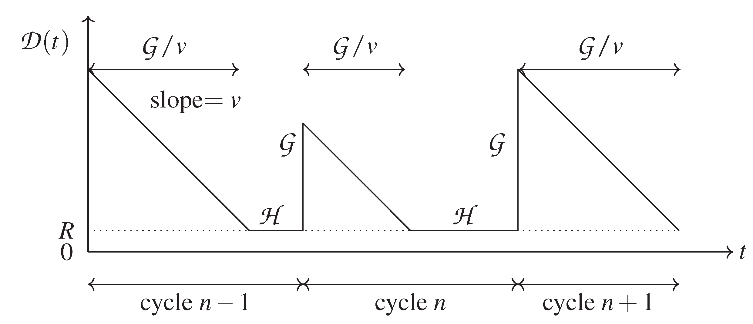
Since the speed is constant, and there are no RSUs, there can be only a single informed cluster on the highway. The dynamics of the system is simple: there are periods in time when only the static message source is aware of the information (the duration of these intervals is represented by exponentially distributed random variable $\mathcal{H}$). As soon as a vehicle enters the radio coverage of the message source, the cluster (of size $\mathcal{G}$) initiated by that vehicle gets informed immediately. Then, this message propagation distance starts decreasing with speed v, and when the last vehicle of the cluster leaves the message source, there will be no informed vehicles on the highway again. The trajectory of the message propagation distance, $\mathcal{D}\left(t\right)$, is depicted by Figure 2.

The transient analysis of the underlying stochastic process is presented by [8], characterizing $F(t,x)=P\left(\mathcal{D}\right(t)>x)$. The information propagation speed itself, however, is not considered in that paper. Nevertheless, the lack of RSUs enables the derivation of it in a simple way. For this system we have that

$$\begin{array}{c}\hfill C=\underset{t\to \infty }{lim}\frac{E\left(\mathcal{G}\right)}{t}=0,\end{array}$$

(4)

where we used the fact that ${lim}_{t\to \infty }F(t,x)={lim}_{t\to \infty }P(\mathcal{D}\left(t\right)>x)=G\left(x\right)$, according to [8], hence, ${lim}_{t\to \infty }E\left(\mathcal{D}\left(t\right)\right)=E\left(\mathcal{G}\right)$. This result is as expected, since the current informed cluster always has to leave the accident before the next cluster can get informed. In the next sections we show that the presence of RSUs leads to essentially different results.

5. Message Propagation Speed in the Presence of RSUs

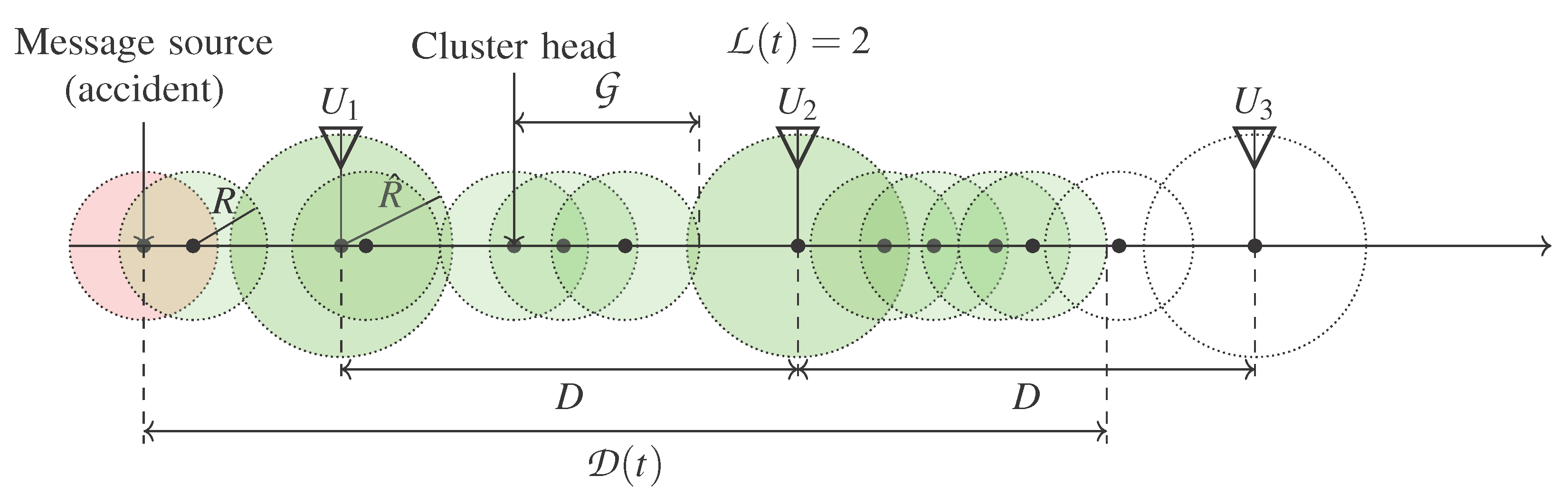
When there are RSUs on the highway as well, a long enough cluster of vehicles can bridge the distance between them, carrying the message from RSU to RSU farther and farther away from the message source. The analysis of the message propagation is based on the observation that the stochastic process $\mathcal{L}\left(t\right)\in \{0,1,\cdots \},t\ge 0$, representing the index of the farthest informed RSU at time t (see Figure 1), is a Markov renewal process.

5.1. $\mathcal{L}\left(t\right)$ as a Markov Renewal Process

In order to derive the asymptotic message propagation speed, we first identify renewal time instants in the evolution of $\mathcal{D}\left(t\right)$, where the process becomes memory-less. There are several such instants, the analysis presented in this paper is based on the time points where the farthest informed RSU, $\mathcal{L}\left(t\right)$, changes. These time points are denoted by ${\mathcal{Q}}_k,k=1,\cdots$, thus ${\mathcal{Q}}_k=t:\mathcal{L}\left(t\right)>\mathcal{L}(t-\Delta )$ for infinitesimally small $\Delta$. It is easy to see that time points ${\mathcal{Q}}_k$ are renewal instants: when an RSU receives the message, it acts as a new message source on the highway.

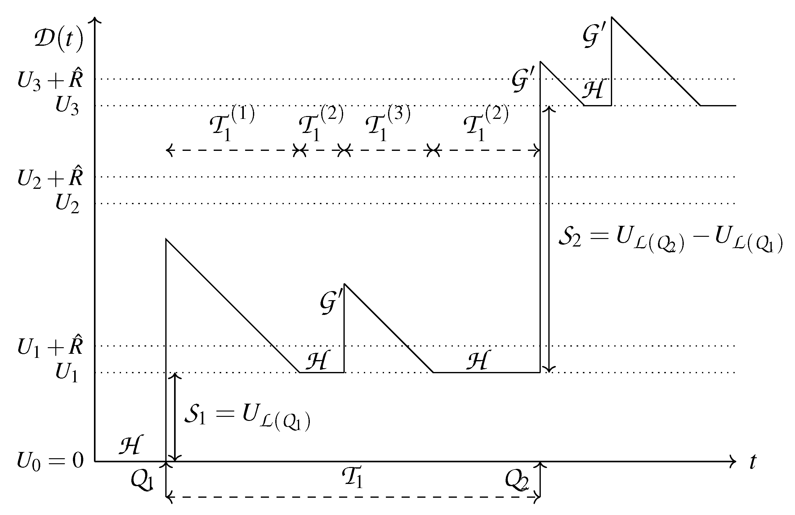
Figure 3 depicts a sample trajectory of $\mathcal{D}\left(t\right)$, where the positions of the RSUs are denoted by $U_k$, $k=1,\cdots$ (to make the figure more compact the distance between the RSUs is not equal here, as opposed to our modeling assumption). Whenever a vehicle enters the coverage of an RSU, a cluster is formed with length ${\mathcal{G}}^{\prime }$. If the cluster is long enough, the message can propagate through several RSUs, marking the next renewal time instant. The distance between the RSU that was the farthest informed previously and the RSU that got the farthest informed at the kth renewal point is denoted ${\mathcal{S}}_k$, hence we have ${\mathcal{S}}_k=U_{\mathcal{L}\left({\mathcal{Q}}_k\right)}-U_{\mathcal{L}\left({\mathcal{Q}}_{k-1}\right)}$.

Some remarks:

• Random variables $\mathcal{G}$ and ${\mathcal{G}}^{\prime }$ are different, since $\mathcal{G}$ measures the length of clusters consisting of vehicles only, while in ${\mathcal{G}}^{\prime }$ the RSUs themselves contribute to the clusters, too.
• Random variables ${\mathcal{T}}_k={\mathcal{Q}}_{k+1}-{\mathcal{Q}}_k,k=1,\cdots$ (the time between renewal instants) and ${\mathcal{S}}_k,k=1,\cdots$ are independent and identically distributed, therefore their subscripts are neglected, they are referred to as $\mathcal{T}$ and $\mathcal{S}$.
• We assume equidistant RSU placement, hence $U_k=k·D$ throughout the paper.
• Following from the definition of $\mathcal{S}$ and the equidistant placement of RSUs, $\mathcal{S}$ is an integer multiple of D.

To make the derivations simpler, we assume that there is an RSU at $U_0$ and that the accident occurs at a renewal point. Since the message propagation speed is an asymptotic quantity, these assumptions do not affect the results. In Section 6, where the transient behavior is studied, the position of the accident is important, and it will be properly taken into account.

The following lemma relates the information propagation speed C and the mean values of $\mathcal{T}$ and $\mathcal{S}$.

Lemma 1.

The information propagation speed C can be computed by

$$\begin{array}{c}\hfill C=\frac{E\left(\mathcal{S}\right)}{E\left(\mathcal{T}\right)}.\end{array}$$

(5)

Proof. 

Let us assume that there are K renewal instants till time t, thus $K=max\{k:{\sum }_{i=1}^k{\mathcal{T}}_i<t\}$. In this case $\mathcal{D}\left(t\right)/t$ can be expressed by

$$\begin{array}{c}\hfill \frac{\mathcal{D}\left(t\right)}{t}=\frac{{\mathcal{S}}_1+{\mathcal{S}}_2+\cdots +{\mathcal{S}}_K+c_S}{{\mathcal{Q}}_1+{\mathcal{T}}_1+{\mathcal{T}}_2+\cdots +{\mathcal{T}}_K+c_T},\end{array}$$

(6)

where ${\mathcal{Q}}_1$ is the time till the first renewal instant, and the terms $c_S$ and $c_T$ are the distance and the time taken since the last renewal point. Observe that $c_S$ is bounded since $c_S<D$ and $c_T$ and ${\mathcal{Q}}_1$ have finite mean values. Taking the limit leads to

$$\begin{array}{cc}\hfill C& =\underset{t\to \infty }{lim}\frac{\mathcal{D}\left(t\right)}{t}=\underset{K\to \infty }{lim}\frac{{\sum }_{k=1}^K{\mathcal{S}}_k+c_S}{{\mathcal{Q}}_1+{\sum }_{k=1}^K{\mathcal{T}}_k+c_T}=\underset{K\to \infty }{lim}\frac{\frac{1}{K}{\sum }_{k=1}^K{\mathcal{S}}_k+\frac{c_S}{K}}{\frac{{\mathcal{Q}}_1}{K}+\frac{1}{K}{\sum }_{k=1}^K{\mathcal{T}}_k+\frac{c_T}{K}}=\frac{E\left(\mathcal{S}\right)}{E\left(\mathcal{T}\right)},\hfill \end{array}$$

(7)

that establishes the Lemma 1. □

5.2. Message Propagation when $\widehat{R}=R$

In the rest of the section we derive $E\left(\mathcal{S}\right)$ and $E\left(\mathcal{T}\right)$ in order to compute C, in the case when the radio coverage of the RSUs equals the radio coverage of the vehicles. This assumption will be relaxed later in Section 5.3.

The next theorem provides $E\left(\mathcal{S}\right)$, which is the mean distance between the farthest informed RSUs when the subsequent vehicles form a long enough cluster and transfer the message to an RSU farther away on the highway (see Figure 3).

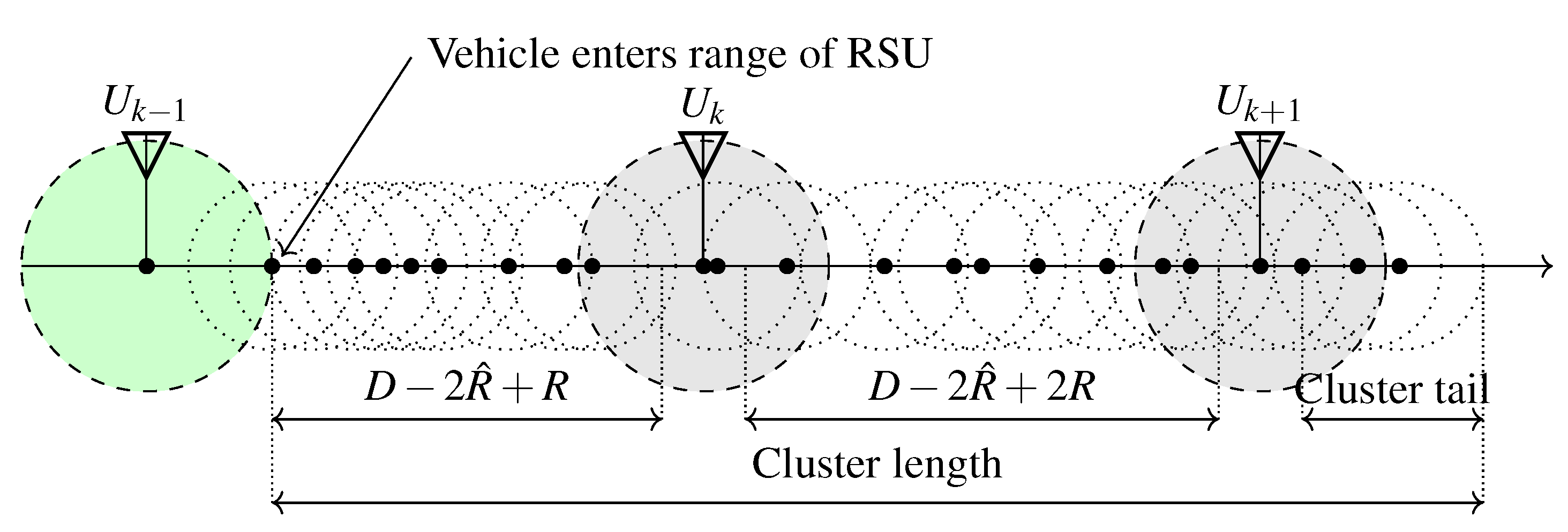
Theorem 1.

The mean distance between the farthest informed RSUs at two subsequent renewal instants, $E\left(\mathcal{S}\right)$, can be obtained by

$$\begin{array}{c}\hfill E\left(\mathcal{S}\right)=\frac{D}{1-G\left(D\right)},\end{array}$$

(8)

where $G\left(x\right)$ is the ccdf of the cluster length given by (2).

Proof. 

A renewal instant occurs when, after an idle period of the farthest informed RSU, a new vehicle arrives with a cluster long enough to reach the next RSU. If the current RSU is located at position $U_{k-1}$, the head of the new cluster enters the range of the RSU at position $U_{k-1}+R$, hence the minimal cluster length reaching the next RSU is $U_k-(U_{k-1}+R)=D-R$ (see Figure 4), consequently, the probability of this event is $G(D-R)$.

The question is, given that the cluster is long enough, implying that a renewal instant occurs, how far does the message get, how many RSUs receive the information at this renewal instant. When this long enough cluster of vehicles reaches the next RSU, the next RSU at $U_k$ acts as a cluster head itself. If this cluster (initiated by the RSU) is longer than D (with probability $G\left(D\right)$), the next RSU gets informed, too, initiating a further cluster, etc. Hence, the number of RSUs receiving the information is geometrically distributed, i RSUs get informed with probability $G{\left(D\right)}^{i-1}(1-G\left(D\right))$. For any two subsequent renewal time instants $Q_1$ and $Q_2$ we have

$$\begin{array}{c}\hfill \begin{array}{cc}\hfill E\left(\mathcal{S}\right)& =\sum _{i=1}^{\infty }i·D·P(\mathcal{L}\left({\mathcal{Q}}_2\right)-\mathcal{L}\left({\mathcal{Q}}_1\right)=i)\hfill \\ & =\sum _{i=1}^{\infty }i·D·G{\left(D\right)}^{i-1}(1-G\left(D\right))=\frac{D}{1-G\left(D\right)},\hfill \end{array}\end{array}$$

that proves (8). □

Our next target towards obtaining C is the derivation of $E\left(\mathcal{T}\right)$. Before the corresponding theorem we need the following lemma enabling the efficient computation of the finite integrals of $G\left(x\right)$.

Lemma 2.

The finite integral of $G\left(x\right)$, defined by $H\left(x\right)={\int }_{y=0}^{x}G\left(y\right)dy$, can be calculated as

$$\begin{array}{c}\hfill H\left(x\right)=\frac{1}{\vartheta }\left(e^{\vartheta R}-1-e^{\vartheta R}G(x+R)\right),\end{array}$$

(9)

for $x>R$.

Proof. 

Let us integrate (2) from 0 to x, for $x>R$. We get

$$\begin{array}{c}\hfill \begin{array}{cc}\hfill H\left(x\right)& ={\int }_{z=0}^{R}1dz+{\int }_{z=R}^x{\int }_{y=0}^R\vartheta e^{-\vartheta y}G(z-y)dydz\hfill \\ & =R+{\int }_{y=0}^R\vartheta e^{-\vartheta y}\underset{H(x-y)}{\underbrace{{\int }_{z=y}^{x}G(z-y)dz}}dy-{\int }_{y=0}^R\vartheta e^{-\vartheta y}\underset{R-y}{\underbrace{{\int }_{z=y}^{R}G(z-y)dz}}dy\hfill \\ & =\frac{1}{\vartheta }(1-e^{-\vartheta R})+{\int }_{y=0}^R\vartheta e^{-\vartheta y}H(x-y)dy.\hfill \end{array}\end{array}$$

(10)

Now we show that (9) satisfies this equation. Inserting (9) into the left-hand side (LHS) of (10) leads to

$$\begin{array}{c}\hfill \frac{1}{\vartheta }\left(e^{\vartheta R}-1-e^{\vartheta R}G(x+R)\right).\end{array}$$

(11)

Inserting (9) into the right-hand side (RHS) of (10) gives

$$\begin{array}{c}\hfill \frac{1}{\vartheta }(1-e^{-\vartheta R})+\frac{1}{\vartheta }\underset{e^{-\vartheta R}+e^{\vartheta R}-2}{\underbrace{{\int }_{y=0}^R\vartheta e^{-\vartheta y}(e^{\vartheta R}-1)dy}}-\frac{1}{\vartheta }{e}^{\vartheta R}\underset{G(x+R)}{\underbrace{{\int }_{y=0}^R\vartheta e^{-\vartheta y}G(x-y+R)dy}}.\end{array}$$

(12)

The LHS and the RHS are matching, proving the Lemma 2. □

Observe that from (9) and (3) we have ${lim}_{x\to \infty }H\left(x\right)=E\left(G\right)$, as expected. The mean time between two renewal instants, $E\left(\mathcal{T}\right)$, is provided by the following theorem.

Theorem 2.

The mean time between two renewal instants can be expressed by

$$\begin{array}{c}\hfill E\left(\mathcal{T}\right)=\frac{\frac{1}{\vartheta }+H(D-R)}{G(D-R)v}+\frac{H\left(D\right)-D}{(1-G(D\left)\right)v}.\end{array}$$

(13)

Proof. 

Let us denote the probability density function of the cluster length $\mathcal{G}$ by $g\left(x\right)={lim}_{\Delta \to 0}\frac{1}{\Delta }P(\mathcal{G}\in (x,x+\Delta ))$, for $x>R$. Random variable $\mathcal{G}$ has a probability mass at point R as well (when the cluster consists of a single element only), thus $P(\mathcal{G}=R)=1-G\left(R\right)$.

Using these notations we can express the three main components of $\mathcal{T}$, denoted by ${\mathcal{T}}^{\left(1\right)},{\mathcal{T}}^{\left(2\right)}$ and ${\mathcal{T}}^{\left(3\right)}$ (see Figure 3), as follows:

• The first component, ${\mathcal{T}}^{\left(1\right)}$ is the departure time of the cluster tail (Figure 4) after the renewal instant. By definition, renewal instants are those time instants when the message gets transferred to farther RSUs. Right after the renewal instant t, the length of the cluster of informed vehicles, measured from RSU $\mathcal{L}\left(t\right)$ (and including this RSU), is $\mathcal{D}\left(t\right)-U_{\mathcal{L}\left(t\right)}$, hence the time till these vehicles leave the RSU (when $\mathcal{D}\left(t\right)$ becomes $U_{\mathcal{L}\left(t\right)}+R$) is ${\mathcal{T}}^{\left(1\right)}=(\mathcal{D}\left(t\right)-U_{\mathcal{L}\left(t\right)}-R)/v$. The mean value of this component can be obtained by

  $$\begin{array}{c}\hfill E\left({\mathcal{T}}^{\left(1\right)}\right)=\frac{(1-G(R\left)\right)·0}{1-G\left(D\right)}+\frac{{\int }_{x=R}^{D}g\left(x\right)\frac{x-R}{v}dx}{1-G\left(D\right)},\end{array}$$

  (14)

  where the first term corresponds to the case when the length of the cluster tail is exactly R (no vehicles are informed beyond the RSU after the renewal instant), implying ${\mathcal{T}}^{\left(1\right)}=0$. The second term covers the case when the length of the cluster tail is $R<x<D$. When the length of the cluster tail (including the RSU) is x, the time till it leaves the RSU is $(x-R)/v$, since this is the time till the cluster length reduces to R, meaning that only the RSU is informed, and no vehicles beyond it. Note that the cluster tail can not be longer than D, since in that case the next RSU would receive the message that contradicts the definition of the cluster tail.
• The second component of $\mathcal{T}$ is the duration of the periods when no vehicles are informed beyond the RSU. These periods are exponentially distributed with parameter $\lambda$, thus

  $$\begin{array}{c}\hfill E\left({\mathcal{T}}^{\left(2\right)}\right)=\frac{1}{\lambda }.\end{array}$$

  (15)
• When there are no informed vehicles beyond the RSU, and a new vehicle enters the range of the RSU, a new cluster gets informed. The position of the first vehicle in this cluster is $U_{\mathcal{L}\left(t\right)}+R$. If the length of the cluster, x, is less than $D-R$, then the message does not reach the next RSU, thus no renewal instant occurs. In this case the time till this cluster leaves the RSU, $x/v$, contributes to $\mathcal{T}$. For the mean value of this component, that is the mean departure time of clusters too short to reach the next RSU, we have

  $$\begin{array}{c}\hfill E\left({\mathcal{T}}^{\left(3\right)}\right)=\frac{(1-G\left(R\right))\frac{R}{v}}{1-G(D-R)}+\frac{{\int }_{x=R}^{D-R}g\left(x\right)\frac{x}{v}dx}{1-G(D-R)}.\end{array}$$

  (16)
  According to the first term the new cluster consists of a single vehicle only; the case when there are more vehicles in the cluster are covered by the second term.

Every renewal period $\mathcal{T}$ starts with component ${\mathcal{T}}^{\left(1\right)}$, followed by ${\mathcal{T}}^{\left(2\right)}$. Then, components ${\mathcal{T}}^{\left(3\right)}$ and ${\mathcal{T}}^{\left(2\right)}$ are repeated as many times as the arriving cluster length turned out to be too short to reach the next RSU, the probability of which is $1-G(D-R)$. When after a ${\mathcal{T}}^{\left(2\right)}$ component a long enough cluster arrives to the RSU, with probability $G(D-R)$, a new renewal instant occurs. We get

$$\begin{array}{c}\hfill E\left(\mathcal{T}\right)=E\left({\mathcal{T}}^{\left(1\right)}\right)+E\left({\mathcal{T}}^{\left(2\right)}\right)+\underset{\frac{1-G(D-R)}{G(D-R)}}{\underbrace{\sum _{i=0}^{\infty }{(1-G(D-R))}^{i}G(D-R)·i}}·(E\left({\mathcal{T}}^{\left(3\right)}\right)+E\left({\mathcal{T}}^{\left(2\right)}\right)).\end{array}$$

(17)

Substituting (14), (15) and (16) into (17) and making use of the relations

$$\begin{array}{cc}\hfill {\int }_{x=R}^{D}g\left(x\right)dx& =G\left(R\right)-G\left(D\right),\hfill \end{array}$$

(18)

$$\begin{array}{cc}\hfill {\int }_{x=R}^{D}xg\left(x\right)dx& =H\left(D\right)-DG\left(D\right)-R(1-G(R\left)\right),\hfill \end{array}$$

(19)

we get

$$\begin{array}{c}\hfill \begin{array}{cc}\hfill E\left(\mathcal{T}\right)& =\frac{{\int }_{x=R}^{D}g\left(x\right)\frac{x-R}{v}dx}{1-G\left(D\right)}+\frac{1}{\lambda }+\frac{(1-G\left(R\right))\frac{R}{v}}{G(D-R)}+\frac{{\int }_{x=R}^{D-R}g\left(x\right)\frac{x}{v}dx}{G(D-R)}+\frac{1-G(D-R)}{G(D-R)}\frac{1}{\lambda }\hfill \\ & =\frac{H\left(D\right)-D}{v(1-G(D\left)\right)}+\frac{D-R}{v}+\frac{1}{\lambda }+\frac{1}{vG(D-R)}(H(D-R)-(D-R)G(D-R))\hfill \\ & \hspace{1em}+\frac{1-G(D-R)}{G(D-R)}\frac{1}{\lambda }\hfill \\ & =\frac{H\left(D\right)-D}{v(1-G(D\left)\right)}+\frac{(D-R)G(D-R)}{vG(D-R)}+\frac{\frac{v}{\lambda }}{vG(D-R)}+\frac{H(D-R)-(D-R)G(D-R)}{vG(D-R)},\hfill \end{array}\end{array}$$

(20)

which equals (13). □

Finally, the main result, the message propagation speed is formulated by the following corollary.

Corollary 1.

The message propagation speed can be calculated by

$$\begin{array}{c}\hfill C=\frac{E\left(\mathcal{S}\right)}{E\left(\mathcal{T}\right)}=v·\frac{D}{\left(\frac{1}{\vartheta }+H(D-R)\right)\frac{1-G\left(D\right)}{G(D-R)}+H\left(D\right)-D}.\end{array}$$

(21)

5.3. Message Propagation when $\widehat{R}>R$

In the practice, the radio coverage of the RSUs is greater than the one of the vehicles, thus $\widehat{R}>R$. In this section we generalize the results obtained above, to this, more realistic scenario.

Theorem 3.

When $\widehat{R}>R$ holds, $E\left(\mathcal{S}\right)$ is computed by

$$\begin{array}{c}\hfill E\left(\mathcal{S}\right)=\frac{D}{1-G(D-2\widehat{R}+2R)}.\end{array}$$

(22)

Proof. 

The proof is similar to the one of Theorem 1. When a vehicle enters the range of the farthest informed RSU (located at $U_{k-1}$) after the renewal instant, the minimal cluster length to reach the coverage of the next RSU is $D-2\widehat{R}+R$ (see Figure 5). If the cluster is longer than that (with probability $G(D-2\widehat{R}+R)$), the next RSU receives the message, a renewal instant occurs, and we have to find out how many RSUs will get the message at this instant.

At this instant, after the RSU at $U_k$ received the message, it starts behaving as a cluster head and the cluster formed by the vehicles close enough to each other can be long enough to reach the next RSU at $U_{k+1}$ as well. The end of this cluster, initiated by the RSU at $U_k$, must be at least $U_{k+1}-\widehat{R}+R$ to pass the message to the next RSU (the position of the last vehicle of the cluster should be greater than $U_{k+1}-\widehat{R}$). However, the ccdf $G\left(x\right)$ characterizing the cluster length we have introduced in (2) assumes that the radio coverage of all cluster elements are the same, it can not take the different radio coverage of the RSU into consideration.

To overcome this technical difficulty, we can observe that the RSU at $U_k$ having radius $\widehat{R}$ can be replaced by an RSU at $U_k+\widehat{R}-R$ having radius R, the distribution of the end position of the cluster generated by them will be exactly the same. Consequently, in this equivalent system the cluster starts at $U_k+\widehat{R}-R$, it must end beyond $U_{k+1}-\widehat{R}+R$, implying that the length must be at least $(U_{k+1}-\widehat{R}+R)-(U_k+\widehat{R}-R)=D-2\widehat{R}+2R$, hence the probability of passing the message to the next RSU is $G(D-2\widehat{R}+2R)$.

As in the proof of Theorem 1, we have

$$\begin{array}{c}\hfill \begin{array}{cc}\hfill E\left(\mathcal{S}\right)& =\sum _{i=1}^{\infty }i·D·P(\mathcal{L}\left({\mathcal{Q}}_2\right)-\mathcal{L}\left({\mathcal{Q}}_1\right)=i)\hfill \\ & =\sum _{i=1}^{\infty }i·D·G{(D-2\widehat{R}+2R)}^{i-1}(1-G(D-2\widehat{R}+2R))=\frac{D}{1-G(D-2\widehat{R}+2R)},\hfill \end{array}\end{array}$$

that equals (8). □

Theorem 4.

When $\widehat{R}>R$ holds, $E\left(\mathcal{T}\right)$ is computed by

$$\begin{array}{c}\hfill E\left(\mathcal{T}\right)=\frac{\frac{1}{\vartheta }+H(D-2\widehat{R}+R)}{G(D-2\widehat{R}+R)v}+\frac{H(D-2\widehat{R}+2R)-D+2\widehat{R}-2R}{(1-G(D-2\widehat{R}+2R))v}.\end{array}$$

(23)

Proof. 

The proof follows the same steps as the one of Theorem 2. The mean values of the three components of the time between two renewal instants, $\mathcal{T}$, depicted in Figure 3, are as follows.

• The mean cluster tail departure time can be obtained as

  $$\begin{array}{c}\hfill E\left({\mathcal{T}}^{\left(1\right)}\right)=\frac{{\int }_{x=R}^{D-2\widehat{R}+2R}g\left(x\right)\frac{x-R}{v}dx}{1-G(D-2\widehat{R}+2R)}.\end{array}$$

  (24)
  The idea behind this formula is the same as we applied in the proof of Theorem 3, hence we replace the RSU at $U_k$ with radius $\widehat{R}$ with an RSU at $U_k+\widehat{R}-R$ with radius R. Since the cluster tail after a renewal instant can not reach the coverage of the next RSU, the cluster must end before $U_{k+1}-\widehat{R}+R$, hence the cluster length must be less than $(U_{k+1}-\widehat{R}+R)-(U_k+\widehat{R}-R)=D-2\widehat{R}+2R$.
• The duration of the periods when there are no informed vehicles beyond the RSU is the same as in case of $\widehat{R}=R$, thus

  $$\begin{array}{c}\hfill E\left({\mathcal{T}}^{\left(2\right)}\right)=\frac{1}{\lambda }.\end{array}$$

  (25)
• The departure time of the clusters that are too short to reach the next RSU is

  $$\begin{array}{c}\hfill E\left({\mathcal{T}}^{\left(3\right)}\right)=\frac{(1-G\left(R\right))\frac{R}{v}}{1-G(D-2\widehat{R}+R)}+\frac{{\int }_{x=R}^{D-2\widehat{R}+R}g\left(x\right)\frac{x}{v}dx}{1-G(D-2\widehat{R}+R)}.\end{array}$$

  (26)
  In this formula, the first term corresponds to the case when the cluster consists of a single vehicle only, and the second term covers the case when the cluster is longer. The maximum cluster length that does not reach the next RSU is $D-2\widehat{R}+R$ (see the proof of Theorem 3).

As in the proof of Theorem 2, the time between renewal instants can be obtained by combining these components, taking $E\left({\mathcal{T}}^{\left(3\right)}\right)+E\left({\mathcal{T}}^{\left(2\right)}\right)$ as many times the cluster of the entering vehicle was too short to transfer the message to the next RSU, thus

$$\begin{array}{c}\hfill E\left(\mathcal{T}\right)=E\left({\mathcal{T}}^{\left(1\right)}\right)+E\left({\mathcal{T}}^{\left(2\right)}\right)+\sum _{i=0}^{\infty }{(1-G(D-2\widehat{R}+R))}^{i}G(D-2\widehat{R}+R)·i·(E\left({\mathcal{T}}^{\left(3\right)}\right)+E\left({\mathcal{T}}^{\left(2\right)}\right)),\end{array}$$

(27)

that, after substitution and algebraic manipulations leads to the theorem. □

From $E\left(\mathcal{S}\right)$ and $E\left(\mathcal{T}\right)$, it is easy to express the speed of the information propagation for the $\widehat{R}\ge R$ case as well.

Corollary 2.

For $\widehat{R}\ge R$ the message propagation speed can be calculated by

$$\begin{array}{c}\hfill C=\frac{E\left(\mathcal{S}\right)}{E\left(\mathcal{T}\right)}=v·\frac{D}{\left(\frac{1}{\vartheta }+H(D-2\widehat{R}+R)\right)\frac{1-G(D-2\widehat{R}+2R)}{G(D-2\widehat{R}+R)}+H(D-2\widehat{R}+2R)-D+2\widehat{R}-2R}.\end{array}$$

(28)

6. Transient Analysis of the Message Propagation

A potential application of VANETs is the propagation of alert messages containing emergency information related to highway accidents. To quantify how efficiently the RSUs and the vehicles disseminate the information, it is important to study the transient properties of the message propagation, thus the probability that the message is available beyond a given RSU after a certain amount of time. In this section we are going to characterize the distribution

$$\begin{array}{c}\hfill L_i\left(t\right)=P(\mathcal{L}\left(t\right)=i|\mathcal{L}\left(0\right)=0),\end{array}$$

(29)

through its Laplace transform

$$\begin{array}{c}\hfill L_i^{*}\left(s\right)={\int }_{t=0}^{\infty }{L}_i\left(t\right)e^{-st}dt,\end{array}$$

(30)

and its double transform

$$\begin{array}{c}\hfill L^{*}(s,z)=\sum _{i=0}^{\infty }{z}^i{\int }_{t=0}^{\infty }{L}_i\left(t\right)e^{-st}dt.\end{array}$$

(31)

In these quantities we implicitly assume that $t=0$ is a renewal point. We will relax this restriction at the end of the section. First we derive the Laplace–Stieltjes transform (LST) of $\mathcal{T}$, the time between two renewal intervals.

Theorem 5.

The Laplace–Stieltjes transform $f^{*}\left(s\right)={\int }_{t=0}^{\infty }{e}^{-st}dP(\mathcal{T}<t)$ can be obtained by

$$\begin{array}{c}\hfill f^{*}\left(s\right)=\frac{\lambda G(D-2\widehat{R}+2R)f_1^{*}\left(s\right)}{s+\lambda -\lambda (1-G(D-2\widehat{R}+2R))f_3^{*}\left(s\right)},\end{array}$$

(32)

where $f_1^{*}\left(s\right)$ and $f_3^{*}\left(s\right)$ are given by (33) and (35), respectively.

Proof. 

As before, in the proof of Theorem 4, we are going to characterize the three components of $\mathcal{T}$ in LST domain separately, then we combine them to get $f^{*}\left(s\right)$.

• The LST of the cluster tail departure time is

  $$\begin{array}{c}\hfill f_1^{*}\left(s\right)=E\left(e^{-s{\mathcal{T}}^{\left(1\right)}}\right)=\frac{1}{1-G(D-2\widehat{R}+2R)}\left({\int }_{x=R}^{D-2\widehat{R}+2R}g\left(x\right)e^{-s\frac{x-R}{v}}dx+1-G\left(R\right)\right).\end{array}$$

  (33)
  Note that in case the length of the cluster tail is exactly R (no vehicles are informed beyond the RSU after the renewal instant), the departure time of the cluster tail is exactly 0, whose Laplace transform is $(1-G\left(R\right))·e^{-0t}=1-G\left(R\right)$, providing the second term in the parenthesis.
• The duration of the “idle” periods, when there are no informed vehicles beyond the RSU, are exponentially distributed with parameter $\lambda$, hence

  $$\begin{array}{c}\hfill f_2^{*}\left(s\right)=E\left(e^{-s{\mathcal{T}}^{\left(2\right)}}\right)=\frac{\lambda }{s+\lambda }.\end{array}$$

  (34)
• The departure time of an arriving cluster that turned out to be too short to reach the next RSU is

  $$\begin{array}{c}\hfill f_3^{*}\left(s\right)=E\left(e^{-s{\mathcal{T}}^{\left(3\right)}}\right)=\frac{1}{1-G(D-2\widehat{R}+R)}\left((1-G\left(R\right))e^{-s\frac{R}{v}}+{\int }_{x=R}^{D-2\widehat{R}+R}g\left(x\right)e^{-s\frac{x}{v}}dx\right).\end{array}$$

  (35)

The renewal intervals always start with a ${\mathcal{T}}^{\left(1\right)}$ and a ${\mathcal{T}}^{\left(2\right)}$ component, and then they have as many ${\mathcal{T}}^{\left(3\right)}$ and ${\mathcal{T}}^{\left(2\right)}$ components as many times the arriving cluster was too short to reach the next RSU. A long enough cluster arriving after a ${\mathcal{T}}^{\left(2\right)}$ component triggers a renewal instant, ending the renewal period. As we have shown before, the number of short clusters is geometrically distributed with parameter $G(D-2\widehat{R}+2R)$, thus we have that

$$\begin{array}{c}\hfill \begin{array}{cc}\hfill f^{*}\left(s\right)& =\sum _{i=0}^{\infty }{(1-G(D-2\widehat{R}+2R))}^{i}G(D-2\widehat{R}+2R)f_1^{*}\left(s\right)f_2^{*}\left(s\right){\left(f_3^{*}\left(s\right)f_2^{*}\left(s\right)\right)}^i\hfill \\ & =\frac{G(D-2\widehat{R}+2R)f_1^{*}\left(s\right)f_2^{*}}{1-(1-G(D-2\widehat{R}+2R))f_3^{*}\left(s\right)f_2^{*}\left(s\right)},\hfill \end{array}\end{array}$$

(36)

from which the theorem follows. We have exploited that the probability density function (pdf) of the sum of random variables has a product form in Laplace transform domain. □

The following theorem and the corresponding corollary provides the Laplace transform and the double transform of the transient distribution.

Theorem 6.

The Laplace transform of the transient distribution $L_i^{*}\left(s\right)$ satisfies the following recursion

$$\begin{array}{c}\hfill L_i^{*}\left(s\right)=\left\{\begin{array}{cc}\sum _{k=1}^i{q}_k{f}^{*}\left(s\right)L_{i-k}^{*}\left(s\right),\hfill & \mathit{for} i>0,\hfill \\ \frac{1}{s}(1-f^{*}\left(s\right)),\hfill & \mathit{for} i=0,\hfill \end{array}\right.\end{array}$$

(37)

where $q_k$ is the probability that k RSUs receive the message at a renewal instant,

$$\begin{array}{c}\hfill q_k=G{(D-2\widehat{R}+2R)}^{k-1}(1-G(D-2\widehat{R}+2R)).\end{array}$$

(38)

Proof. 

Assuming that $t=0$ is a renewal instant and conditioning on the time till the next renewal instant leads to

$$\begin{array}{c}\hfill P(\mathcal{L}\left(t\right)=i|{\mathcal{T}}_1=\tau )=\left\{\begin{array}{cc}{\delta }_{i,0},\hfill & t<\tau ,\hfill \\ \sum _{k=1}^i{q}_k{L}_{i-k}(t-\tau ),\hfill & t>\tau .\hfill \end{array}\right.\end{array}$$

(39)

In the first case, when t is before the renewal instant $\tau$, only RSU 0 has the message, as represented by the Kronecker delta, for which ${\delta }_{i,0}=1$ holds if $i=0$ and it is ${\delta }_{i,0}=0$ otherwise. In the second case there was a renewal instant at time $\tau$ when k RSUs received the message, thus, in the remaining time $t-\tau$, $k-i$ further RSUs need to receive the message. The probabilities $q_k$ follow from the proof of Theorem 3.

After deconditioning (39) with the pdf of ${\mathcal{T}}_1$, $f\left(t\right)$, we get

$$\begin{array}{c}\hfill L_i\left(t\right)={\delta }_{i,0}{\int }_{\tau =t}^{\infty }f\left(\tau \right)d\tau +\sum _{k=1}^i{q}_k{\int }_{\tau =0}^{t}f\left(\tau \right)L_{i-k}(t-\tau )d\tau ,\end{array}$$

(40)

which, after Laplace transformation, provides (37). □

Corollary 3.

The double transform of the transient distribution, $L^{*}(s,z)$, is explicitly given by

$$\begin{array}{c}\hfill L^{*}(s,z)=\frac{(1-zG(D-2\widehat{R}+2R))(1-f^{*}\left(s\right))}{s(1-zG(D-2\widehat{R}+2R))-sz{f}^{*}\left(s\right)(1-G(D-2\widehat{R}+2R))}.\end{array}$$

(41)

Proof. 

Applying the definition of $L^{*}(s,z)$ on (37) yields

$$\begin{array}{c}\hfill \begin{array}{cc}\hfill L^{*}(s,z)& =\sum _{i=0}^{\infty }{z}^i{L}_i^{*}\left(s\right)=\frac{1}{s}(1-f^{*}\left(s\right))+\sum _{i=1}^{\infty }{z}^i\sum _{k=1}^i{q}_k{f}^{*}\left(s\right)L_{i-k}^{*}\left(s\right)\hfill \\ & =\frac{1}{s}(1-f^{*}\left(s\right))+f^{*}\left(s\right)\sum _{k=1}^{\infty }{z}^k{q}_k\sum _{i=k}^{\infty }{z}^{i-k}{L}_{i-k}^{*}\left(s\right)\hfill \\ & =\frac{1}{s}(1-f^{*}\left(s\right))+f^{*}\left(s\right)q\left(z\right)L^{*}(s,z),\hfill \end{array}\end{array}$$

(42)

where $q\left(z\right)$ is the probability generating function of $q_k$,

$$\begin{array}{c}\hfill q\left(z\right)=\sum _{k=1}^{\infty }{z}^{k}G{(D-2\widehat{R}+2R)}^{k-1}(1-G(D-2\widehat{R}+2R))=\frac{z-zG(D-2\widehat{R}+2R)}{1-zG(D-2\widehat{R}+2R)}.\end{array}$$

(43)

Expressing $L^{*}(s,z)$ from (42) gives (41). □

Typically, $t=0$ is not a renewal point, for example because there are no vehicles in the range of the highway accident initially, or because the distance between the accident and the first RSU is not D. In this case we have to treat the time interval till the first renewal point differently, which leads to a slightly different result for the double transform (see (42)),

$$\begin{array}{c}\hfill {\widehat{L}}^{*}(s,z)=\frac{1}{s}(1-{\widehat{f}}^{*}\left(s\right))+q\left(z\right){\widehat{f}}^{*}\left(s\right)L^{*}(s,z),\end{array}$$

(44)

where the quantities denoted by a hat correspond to the initial time interval that do not start with a renewal point. Here, the special nature of the first interval is captured solely by ${\widehat{f}}^{*}\left(s\right)$. For instance, if there are no vehicles in the range of the accident, the distance to the first RSU is $D^{\prime }>R$, and the radio coverage of the message source is R, ${\widehat{f}}^{*}\left(s\right)$ can be calculated by

$$\begin{array}{c}\hfill {\widehat{f}}^{*}\left(s\right)=\frac{\lambda G\left(D^{\prime }\right)}{s+\lambda -\lambda (1-G\left(D^{\prime }\right)){\widehat{f}}_3^{*}\left(s\right)},\end{array}$$

(45)

where

$$\begin{array}{c}\hfill {\widehat{f}}_3^{*}\left(s\right)=\frac{1}{1-G(D^{\prime }-R)}\left((1-G\left(R\right))e^{-s\frac{R}{v}}+{\int }_{x=R}^{D^{\prime }-R}g\left(x\right)e^{-s\frac{x}{v}}dx\right),\end{array}$$

(46)

based on the proof of Theorem 5. In general, the proof of Theorem 5 provides guidance to derive the time till the first renewal point ${\widehat{f}}^{*}\left(s\right)$, from which the double transform of the transient distribution is given by (44).

7. Numerical Examples

In this section, we investigate the alert message dissemination in VANET in the presence of RSUs in different scenarios. In the first scenario the radio range of the RSU and the vehicles are the same ($\widehat{R}=R$), while in the second scenario the radio ranges are different. The implementation of the analytical method is based on Matlab (Matlab R2018b, MathWorks, Natick, MA, USA). To verify the results, we also developed a custom simulation tool in C++ language. This simulation tool models the system at the same level of details as the analytical model. It is based on the discretization of the time axis, it updates the position of the vehicles every $0.001$ s. We stopped the simulation after considering 2 million vehicles. Decreasing the time step or increasing the number of vehicles further did not change the results significantly. Nevertheless, we note that our results are exact, the only purpose of the simulation is to validate the correctness of our Matlab implementation. The analytical and simulation methods gave essentially the same results in all of the different scenarios, as shown by the plots in Section 7.1 and Section 7.2, where the lines correspond to the analytical, and the marks to the simulation results. We note that in many cases the simulation is very slow, while the analytical method gives prompt results.

In all of the numerical examples, the vehicle speed is assumed to be v = 36 m/s, which is a common speed limitation for highways in several countries.

7.1. RSU and Vehicle Have the Same Radio Range $\widehat{R}=R$

In this subsection the transmission range of both the RSUs and the vehicles is set to $\widehat{R}=R$ = 150 m. In each forthcoming figure in this section we present two plots. On the left the radio coverage is fixed to R = 150 m, and different arrival rate values are considered, $\lambda \in \{0.45,0.65,0.95\}$. On the right the arrival rate is fixed to $\lambda =0.65$, and two different radio coverages are investigated, $R\in \{150$ m, 250 m}.

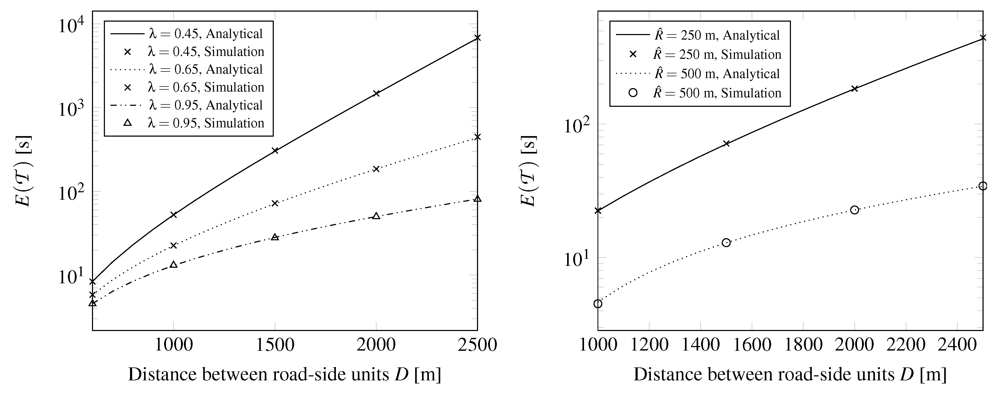
Figure 6 depicts the mean time between two renewal instants $E\left(\mathcal{T}\right)$ (the mean time the message is passed to RSUs farther away), according to Theorem 2. As expected, increasing the RSU distance D increases $E\left(\mathcal{T}\right)$ as well. At higher traffic rate the clusters are longer, thus the message can reach the next RSUs sooner. The radio range of the vehicles and RSUs, R has a big impact on $E\left(\mathcal{T}\right)$, as shown on the right side of Figure 6.

Figure 7 depicts $E\left(\mathcal{S}\right)$, the mean distance between the RSU that was the farthest informed previously and the RSU that got the farthest after getting informed at a renewal instant. According to Figure 7 the relation between D and $E\left(\mathcal{S}\right)$ is not monotonous. If D is small, more RSUs can get the message when a long enough cluster arrives. If D is big, a lot of time is needed to transfer the message from an RSU to an other one, but once it occurs, the distance the message moved forward is greater. Increasing transmission range R can increase the mean distance as shown on the right side of Figure 7.

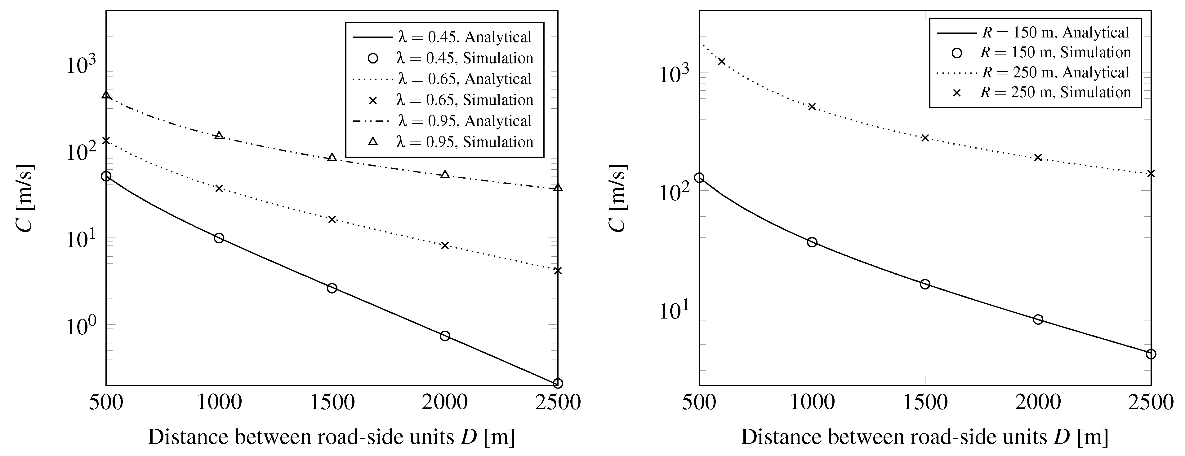
The ratio of $E\left(\mathcal{S}\right)$ and $E\left(\mathcal{T}\right)$ gives the speed C, depicted in Figure 8. Greater radio coverage and greater traffic intensity leads to higher message propagation speed. Observe that at $R=250$ and with appropriate RSU distance the message propagation speed can be very high, much higher than the speed of counter-flow vehicles. These curves are useful to find the optimal distance when planning the RSU deployment.

7.2. RSU and Vehicle with Different Radio Range $\widehat{R}\ne R$

In many published papers [15,16,17] regarding the RSU deployment, the radio range of vehicles and RSUs are the same. We extended our investigation to the case of different radio ranges for vehicles and RSUs, which is more realistic, since RSUs have more powerful radio equipment. In this section we study two different radio coverage values for the RSUs, $\widehat{R}\in \{$250 m, 500 m}.

As shown on the right side of Figure 9, increasing the radio range of the RSUs by a factor of 2 decreases $E\left(\mathcal{T}\right)$ by at least one order of magnitude. The left side of Figure 9 is similar to the results with the same ranges (Figure 6), there is some improvement due to the greater $\widehat{R}$.

Figure 10 depicting $E\left(\mathcal{S}\right)$ is similar to Figure 7, the same non-monotonous behavior can be observed here, too. Due to the greater $\widehat{R}$, $E\left(\mathcal{S}\right)$ is greater in this case.

According to the right side of Figure 11, the greater radio coverage of the RSU has a big impact on the message propagation speed. On the left side of Figure 11, the speed values got improved compared to the $\widehat{R}=R$ case.

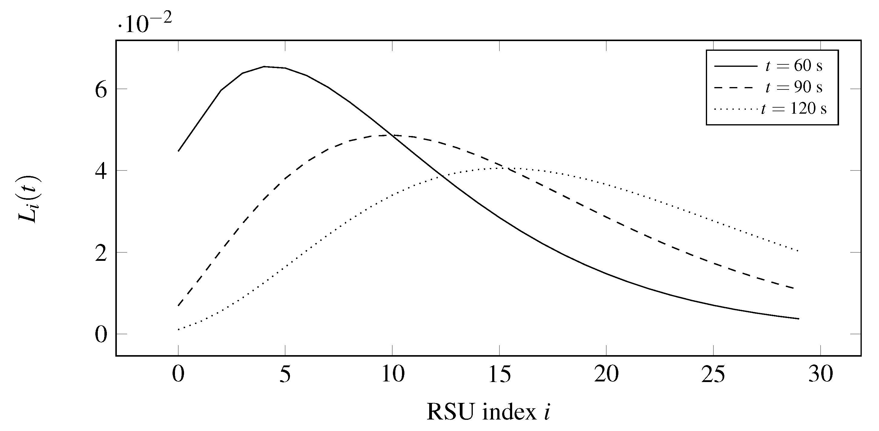
7.3. Transient Distribution of the Farthest Informed RSU

The results of Section 6 make it possible to investigate which is the farthest RSU having the message received at time t. To this end, we computed the Laplace transforms $L_i^{*}\left(s\right)$ for $i=0,\cdots ,30$ using (37) and applied the CME-based inverse Laplace transform method [29] to get the results in time domain. We have set the parameters to $\widehat{R}=R$ = 250 m, $D=D^{\prime }$ = 1500 m in this experiment. The distributions are depicted by Figure 12. According to Figure 12, after 60 s it is most likely that RSU number 4 is the farthest informed RSU, after 90 s it is RSU number 10 and after 120 s it is RSU number 15.

7.4. Discussion of the Results

Based on the results presented above we can conclude that the dependence of the message propagation speed on parameters $D,\lambda$ and R is rather complex. In general, greater distance D, lower traffic rate $\lambda$ and smaller radio coverage R lead to slower message propagation speed, although their relation is far not linear. We also demonstrated that the radio coverage of the RSU, $\widehat{R}$, also has a big impact on the message propagation speed, by the appropriate setting of the D and $\widehat{R}$ parameters the message propagation can be very fast, well above 100 m/s.

In order to optimize the placement of the RSUs one has to determine the greatest distance D by which the quality of service (QoS) parameters are satisfied. Based on the results presented in this paper the criteria can be

• that the message propagation speed exceeds a minimal acceptable value,
• or that the probability that the message reaches a given RSU in a certain amount of time exceeds a threshold.

8. Conclusions

Relying on the Markov renewal process embedded at those instants where the message gets delivered to further RSUs we were able to derive the asymptotic speed of the message propagation, also in the case when the radio coverage of the vehicles and the RSUs are different. The corresponding formula is explicit, quite compact, and easy to evaluate. According to our numerical investigations with realistic parameters we found that with the proper placement of RSUs it is possible to achieve very high message propagation speed, much higher than the speed of the vehicles of the counter-flow traffic. The results of this paper can be used in the network planning process of VANETs with disconnected RSUs.