Mathematical Modeling Shows That the Response of a Solid Tumor to Antiangiogenic Therapy Depends on the Type of Growth

Abstract

It has been hypothesized that solid tumors with invasive type of growth should possess intrinsic resistance to antiangiogenic therapy, which is aimed at cessation of the formation of new blood vessels and subsequent shortage of nutrient inflow to the tumor. In order to investigate this effect, a continuous mathematical model of tumor growth is developed, which considers variables of tumor cells, necrotic tissue, capillaries, and glucose as the crucial nutrient. The model accounts for the intrinsic motility of tumor cells and for the convective motion, arising due to their proliferation, thus allowing considering two types of tumor growth—invasive and compact—as well as their combination. Analytical estimations of tumor growth speed are obtained for compact and invasive tumors. They suggest that antiangiogenic therapy may provide a several times decrease of compact tumor growth speed, but the decrease of growth speed for invasive tumors should be only modest. These estimations are confirmed by numerical simulations, which further allow evaluating the effect of antiangiogenic therapy on tumors with mixed growth type and highlight the non-additive character of the two types of growth.

1. Introduction

The use of mathematical methods has currently become a necessity in oncology. The identification of tumor cells [1], the design of nanomedical systems [2], and real-time adaptation of radiotherapy [3] are just a few examples of problems for which the solution already benefits from the use of simulation studies. One specific mathematical approach is the modeling of tumor growth and treatment, wherein a whole tumor and its microenvironment are considered as a single complex system. Its main goals are gaining new insights into various aspects of cancerous tumors [4,5] and the suggestions for the optimization of treatment protocols [6,7].

Clearly, a mathematical model of tumor growth must capture at least some of the most essential features of cancer cells’ behavior and their interaction with the microenvironment. The most notable property of cancer cells is their ability for unlimited growth under favorable conditions [8]. However, tumor growth in tissue is restrained, first of all by the limited availability of nutrients. These aspects were taken into consideration already in the first non-spatially distributed phenomenological models of tumor growth [9,10]. Accounting for another hallmark of cancer—tissue invasion and metastasis—is possible in models that explicitly consider the spatial distribution of cancer cells. In continuous models, the intergrowth of tumor in normal tissue is usually realized via the introduction of parabolic terms, which include the intrinsic motility of tumor cells as a parameter [11,12]. As a rule, these models neglect the convective motion, which arises due to the proliferation of tumor cells. This process by itself can provide an increase in tumor volume even under zero cell motility. Accounting for it can be realized via hyperbolic equations and by itself results in a compact type of tumor growth [13,14]. Such a mechanism is often crucial for low-grade tumors, while the invasive type of growth usually begins to play an increasing role during their progression.

One more hallmark of cancer is sustained angiogenesis, i.e., the formation of new blood vessels that leads to an increase in tumor nutrient supply and thus promotes its growth. This process was incorporated in various ways in mathematical models of different complexity, from the ones governed by ordinary differential equations [15,16], to the complicated multiscale hybrid models [17,18].

The first antiangiogenic drug, bevacizumab, was approved for medical use in 2004 and is utilized currently along with about a dozen other angiogenesis inhibitors. Today, the majority of approved administration schemes, which include antiangiogenic drugs, combine them with various chemotherapeutic agents, which are aimed at direct cell killing [19]. Early experiments on mouse tumor models showed promising results regarding the use of antiangiogenic drugs in monotherapy regimes as well, since their administration as single agents allowed achieving significant delays in tumor growth. However, in the majority of the clinical trials, the administration of mono-AAT did not lead to any notable increase in survival [20]. Such a discrepancy is supposed to be linked to one obvious qualitative difference between preclinical and clinical tests: while the former were mostly conducted on localized primary tumors, the latter were mainly focused on the late-stage diseases [21]. Only relatively recently have clinical trials for early-stage localized tumors been initiated. Their preliminary data suggest the efficiency of mono-AAT for such tumors, at least in terms of tumor mass reduction [22].

Various mechanisms of resistance to treatment have been proposed in order to explain this effect [23]. One such mechanism is the accentuated invasiveness of tumor cells, which allows them to move away from nutrient-deprived zones. There exists a significant amount of experimental evidence that AAT accelerates tumor progression towards increasingly invasive phenotypes [21,24]. Based on this observation, it has been hypothesized that the tumors, which initially have an invasive phenotype, should possess intrinsic resistance to AAT, while compactly growing tumors should be more susceptible to it [23].

In this work, a continuous model of a monoclonal tumor growth in tissue is presented, which is able to reproduce this effect. The model allows accounting for both types of tumor growth, as well as their combination. Analytical estimations of tumor growth speed are obtained for tumors with both of the pure types of growth, which allow assessing the effect of antiangiogenic therapy on them. Numerical simulations are presented, which show good agreement with analytical estimations. They further allow evaluating the effect of antiangiogenic therapy on tumors with a mixed type of growth and provide insights into the mechanism of the interaction between the two types of growth, highlighting their non-additive character.

2. Model

2.1. Equations

The mathematical model of tumor growth, considered herein, represented a simplification of the model, previously developed by our research group. Its different versions were used for the investigation of several aspects of tumor growth and treatment [25,26,27]. There were four variables in this version of the model, which were a function of space and time coordinates, x and t: the density of tumor cells $n(x,t)$, the fraction of necrotic tissue $m(x,t)$, the concentration of glucose $g(x,t)$, and the density of capillaries surface area $c(x,t)$. All the variables, as well as all the used parameters should be strictly non-negative due to their physical meaning. The one-dimensional planar case was considered in this work, which was suitable for the consideration of a large spherically-symmetrical tumor. The following set of equations governs the dynamics of the model variables:

$$\begin{array}{cc}\hfill \mathrm{tumor}\mathrm{cells}:& \frac{\partial n}{\partial t}=\stackrel{\mathrm{proliferation}}{\overbrace{Bn·[1-\sigma (g\left)\right]}}\stackrel{\mathrm{death}}{\overbrace{-Mn·\sigma \left(g\right)}}\stackrel{\mathrm{migration}}{\overbrace{+D_n\frac{{\partial }^{2}n}{\partial x^2}}}\stackrel{\mathrm{convection}}{\overbrace{-\frac{\partial \left(\mathbf{I}n\right)}{\partial x}}};\hfill \\ \hfill \mathrm{necrotic}\mathrm{tissue}:& \frac{\partial m}{\partial t}=\stackrel{\mathrm{death}}{\overbrace{Mn·\sigma \left(g\right)}}\stackrel{\mathrm{convection}}{\overbrace{-\frac{\partial \left(\mathbf{I}m\right)}{\partial x}}};\hfill \\ \hfill \mathrm{glucose}:& \frac{\partial g}{\partial t}=\stackrel{\mathrm{inflow}}{\overbrace{Pc[1-g]}}\stackrel{\mathrm{consumption}}{\overbrace{-Qn·[1-\sigma (g\left)\right]}}\stackrel{\mathrm{diffusion}}{\overbrace{+D_g\frac{{\partial }^{2}g}{\partial x^2}}};\hfill \\ \hfill \mathrm{capillaries}:& \frac{\partial c}{\partial t}=\stackrel{\mathrm{degradation}}{\overbrace{-R[n+m]c}};\hfill \\ \hfill where& \sigma \left(g\right)=\frac{1}{2}[1-\tanh (\epsilon \{g-g_{cr}\}\left)\right];\hfill \\ & \nabla \mathbf{I}=Bn·[1-\sigma (g\left)\right]+D_n\frac{{\partial }^{2}n}{\partial x^2}.\hfill \end{array}$$

(1)

2.1.1. Tumor Cells

The term tumor cell proliferation implies that it happens ceaselessly under a sufficient level of glucose, which was chosen to be the key nutrient, since it is indispensable for cell division [28]. With the fall of glucose level, the rate of proliferation slows down, and tumor cells die by necrosis. The drainage of necrotic tissue was neglected. The exact rates of the processes of cell proliferation and death were governed by a sigmoid function $\sigma \left(g\right)$. Tumor cells were able to migrate throughout the tissue, which was governed by a diffusion-like term. The convective terms described the bulk motion of tissue elements, the velocity field $\mathbf{I}$ being determined by the dynamics of tumor cells. The expression for it was derived under the assumption of the constancy of the total density of tumor cells, necrotic tissue, and normal cells, which was normalized to unity. The normal cells were not considered in the model explicitly; however, it was assumed that the passive motion due to the arising convective flow was the only part of their dynamics.

2.1.2. Glucose and Capillaries

The dynamics of glucose is comprised of its inflow from the capillaries into the tissue, consumption by tumor cells, and diffusion throughout the tissue. The inflow of glucose is governed primarily by the process of passive diffusion through the walls of capillaries [29]. Therefore, the rate of glucose inflow is proportional to the density of the capillaries’ surface area and to the difference in glucose concentrations in blood and in tissue. Glucose concentration in blood was considered to be constant and was normalized to unity.

The capillary network degrades inside the tumor. This process has various reasons of a mechanical [30] and chemical nature [31], the details of which are difficult to account for in a reliable manner. Therefore, the degradation of capillaries was described by a rather phenomenological term. The volume of capillaries was considered to be negligible compared to the volume of cells, and therefore, their dynamics did not affect the convective velocity field. The convective motion of capillaries was also neglected. The normal density of capillaries’ surface area was normalized to unity.

2.1.3. Angiogenesis and Antiangiogenic Therapy

A more or less straightforward consideration of angiogenesis would require the introduction of an additional variable for the concentration of the main pro-angiogenic factor VEGF, which would affect the dynamics of capillaries. Such an approach has been utilized previously in different continuous models of tumor growth [12,32,33], including our models [27,34]. Herein, a more concise method was used for the sake of analytical study. It was assumed that during the growth of an untreated tumor, the concentration of VEGF was so high that it provided the maximum possible angiogenic effect throughout all the considered part of the tissue (the rate of this effect was limited by the number of receptors on endothelial cells). In fact, there are two separate effects, induced by VEGF, that affect the inflow of glucose from the capillaries and therefore needed to be considered in this model. One of them is the increase of the capillary density due to the formation of new capillaries. Another effect is the increase of the vascular permeability [35,36]. Due to the above-described assumption of the uniform action of VEGF, accounting for the latter effect came down to the increase in the value of parameter P, since it corresponded to the uniform identical increase in the permeability of all capillaries in the tissue. Assuming further that the local increase of the capillaries’ surface area density, c, was proportional to its own local value throughout the tissue, one may conclude that for the consideration of the glucose inflow in tissue, an increase of c was equivalent to an analogous increase in the value of parameter P. Thus, the total effect of angiogenesis was accounted for in this model by the increase in the value of a single parameter P. Since AAT leads to the normalization of the structure of capillaries and further normalization of their density [37,38], its action as reflected by a decrease of P to a value, which was assumed to correspond to normal tissue.

2.2. Parameters

The parameters of the model were estimated according to the data of various experimental works. The basic set of parameters is listed in

Table 1. Basic set of model parameters.

Parameter	Description	Estimated Value	Model Value	Based on
B	tumor cells’ proliferation rate	0.01 h${}^{-1}$	0.01	[39]
Q	tumor cells’ glucose consumption rate	$6.2\times {10}^{-17}$ mol/(cells·s)	12	[39]
$D_g$	glucose diffusion coefficient	$2.8\times {10}^{-6}$ cm${}^2$/s	100	[42]
P	angiogenesis parameter	$1.1\times {10}^{-5}$ cm/s	4	[29]
$g_{cr}$	critical level of glucose	0.56 mM	0.1	see the text
$D_n$	tumor cells’ motility	$2.4\times {10}^{-4}$ cm${}^2$/day	0.1	[40]
M	tumor cells’ death rate	0.05 h${}^{-1}$	0.05	see the text
R	capillaries’ degradation rate	$1.7\times {10}^{-10}$ mL/(cells·s)	0.2	[41]
$ϵ$	tumor cells’ sensitivity to glucose level	–	100	see the text

. The dimensionless model values of the parameters were the approximations of their normalized values, which were obtained with the use of the following normalization parameters: $t_n=1$ h for time, $x_n={10}^{-2}$ cm for length, $g_n=1$ mg/mL for glucose concentration, $c_n=100{\mathrm{cm}}^2/{\mathrm{cm}}^3$ for normal capillary surface area density, which was close to its average value for human muscle [29], and $n_n=3\times {10}^8$ cells/mL for the maximum density of tumor cells. The latter value was taken from the experimental work on the in vitro growth of multicellular tumor spheroids [39]. The values for the proliferation rate of tumor cells and their glucose consumption rate were also estimated according to the data of this work; however, it was assumed that these values should be proportionally diminished during the growth of a relevant tumor in tissue. The basic coefficient of tumor cells’ motility corresponded to highly motile glioma cells [40]. This parameter is set to zero in Section 3.1 in order to focus on the compact type of tumor growth and is varied in Section 3.3 in order to consider tumors with a mixed type of growth. The value for capillaries’ degradation rate was chosen in order to correspond to experimental observations, which showed that capillaries with adequate blood filling were very scarce inside the core of the tumors with radii of several millimeters [41]. The rate of death of tumor cells was taken to be significantly higher that that of their proliferation. The values of the parameters of function $\sigma \left(g\right)$ could not be assessed straightforwardly, since the form of this function was chosen for phenomenological reasons. Therefore, it was merely taken to be rather close to a stepwise function, with the transition of tumor cells from proliferation to death happening at the concentrations of glucose an order of magnitude lower than that in blood. Importantly, the use of these values of variables M, $g_{cr}$, and $ϵ$ allowed keeping the concentrations of glucose positive within the necrotic zone.

In order to consider the effect of angiogenesis on tumor growth, the value of angiogenesis parameter P was varied up to a value ten times greater than the basic one. Such a limit was selected as a very approximate product of two estimated factors. Firstly, experiments in various mouse tumor models showed that the local density of microvessels near a tumor could increase three to six times [43]. Secondly, in the work [34], it was shown that a 2.5-fold increase in the permeability of tumor capillaries to glucose due to the action of VEGF was a physiologically reasonable estimation.

2.3. Numerical Solving

During numerical simulations, the set of equations Equation (1) was solved in a region with a size of several centimeters. The exact size X was adjusted for each case in order to be sufficiently small to spare computational time without imposing noticeable edge effects, while for all the variables, the zero-flux boundary condition was used at both edges. The convective flow speed was set to zero at the left boundary, where $x=0$, resulting in the following equation for it:

$${\displaystyle \mathbf{I}(x,t)={\int }_0^{x}Bn(r,t)·[1-\sigma \left(g(r,t)\right)]\mathrm{d}r+D_n\frac{\partial n(x,t)}{\partial x}.}$$

The following initial conditions were used, which represented a normal tissue with a small, 0.01 mm in width, colony of tumor cells, located near the left boundary, where capillaries were absent:

$$\begin{array}{cccc}\left\{\begin{array}{c}n=1,\\ m=0,\\ g=1,\\ c=0\end{array}\right.\hfill & \hfill forx<=0.1;& \left\{\begin{array}{c}n=0,\\ m=0,\\ g=1,\\ c=1\end{array}\right.\hfill & \hfill forx>0.1.\end{array}$$

(2)

The method of splitting into physical processes was used for all variables, i.e., kinetic equations, diffusion equations, and convective equations were solved successively during each time step. The implicit Crank–Nicholson scheme was used for the glucose diffusion equation. Since the glucose diffusion term provided maximum rate of local change among all the variables and thus required a sufficiently small time step even for implicit solving, it was decided to solve the cell migration equation by a simpler explicit forward Euler scheme, and all kinetic equations by the explicit Euler method. Convective equations were solved using the flux-corrected transport algorithm with explicit anti-diffusion stage. The last method was introduced in the work [44], while other classical methods were described in many books (see, e.g., [45]). The choice of time and space steps is justified in the following sections. For optimization purposes, the function $\sigma \left(g\right)$ was not recalculated every time; instead, it was precalculated for about ten thousand values of g, evenly distributed on the segment $[0,1]$, and only thusly obtained values were used during the calculations as approximations of the actual values of $\sigma \left(g\right)$.

The tumor growth speed $V_{gr}\left(t\right)$ was calculated as the rate of change of tumor radius, which was evaluated as the maximum space coordinate, at which $n\ge 0.1$. In all the simulations, after an initial transitional period, the speed of tumor growth seemed to tend asymptotically to some constant value. In order to ensure that this value could be estimated with suitable precision, for each simulation, the part of the function $V\left(t\right)$, obtained after the manually designated initial transitional period, was fitted via the least-squares method by a function of the form:

$$V_{gr}\left(t\right)=V+\sum _{i=1}^k{a}_i{e}^{-b_{i}t},$$

wherein the value $k=3$ was selected manually as the one providing sufficiently fine approximation. A simulation was stopped manually if the current tumor growth speed and V, expressed in mm/week, were equal up to three decimal places. If it did not happen until the proximity of the tumor to the right boundary notably affected its growth speed, the simulation was rerun in a larger region. Further throughout the text, this limiting value V is meant for tumor growth speed.

For some simulations, the number of tumor cells was estimated analogically as:

$$N=\underset{t\to \infty }{lim}{\int }_0^{X}n\left(x\right)dx,$$

the integral being calculated numerically by the elementary rectangle rule.

The computational codes were implemented in C++ and can be found in the Supplementary Materials.

3. Results

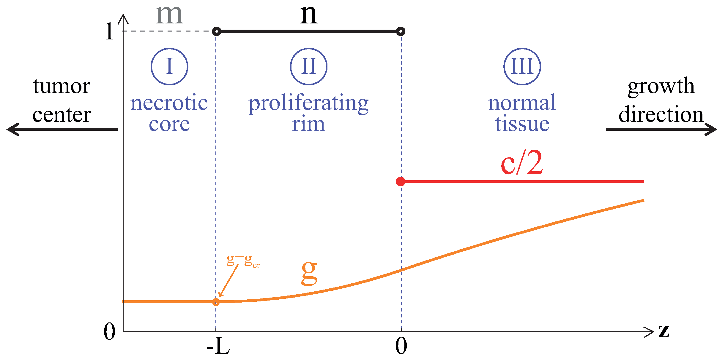
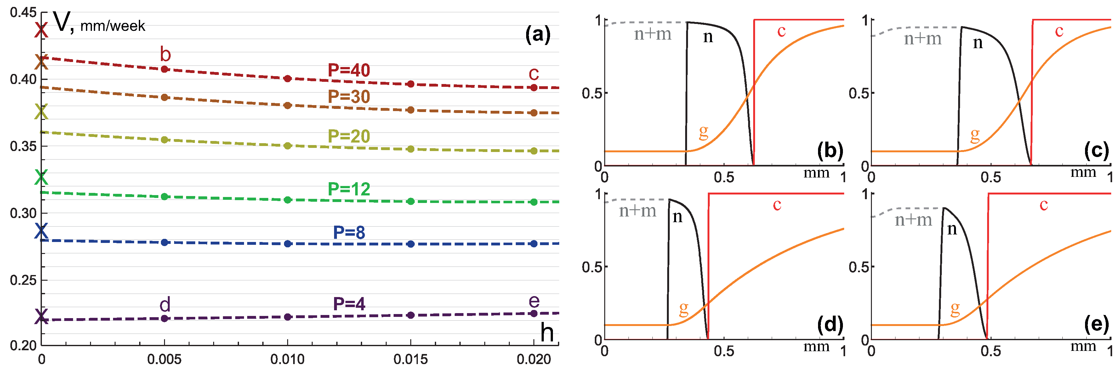
3.1. Compact Type of Growth

At first, let us obtain an analytical estimation for the growth speed of a solid tumor with zero cell motility, i.e., $D_n=0$, which thus has a purely compact type of growth. For this purpose, let us seek the solution of Equation (1) in the form of a wave, traveling with constant shape and speed V in an infinite region. In such a case, the governing equations can be reduced to a system of ordinary differential equations by introducing the traveling coordinate frame $z=x-Vt$:

$$\begin{array}{cc}\hfill \mathrm{tumor}\mathrm{cells}:& Bn·[1-\sigma \left(g\right)]-Mn·\sigma \left(g\right)-\frac{\partial \left(\mathbf{I}n\right)}{\partial z}+V\frac{\partial n}{\partial z}=0;\hfill \\ \hfill \mathrm{necrotic}\mathrm{tissue}:& Mn·\sigma \left(g\right)-\frac{\partial \left(\mathbf{I}m\right)}{\partial z}+V\frac{\partial m}{\partial z}=0;\hfill \\ \hfill \mathrm{glucose}:& Pc[1-g]-Qn·[1-\sigma \left(g\right)]+D_g\frac{{\partial }^{2}g}{\partial z^2}+V\frac{\partial g}{\partial z}=0;\hfill \\ \hfill \mathrm{capillaries}:& -R[n+m]c+V\frac{\partial c}{\partial z}=0;\hfill \\ \hfill where& \sigma \left(g\right)=\frac{1}{2}[1-\tanh (\epsilon \{g-g_{cr}\}\left)\right];\hfill \\ & \mathbf{I}\left(z\right)={\int }_{-\infty }^{z}Bn\left(r\right)·[1-\sigma (g\left(r\right)\left)\right]\mathrm{d}r;\hfill \\ & V=\underset{z\to +\infty }{\lim }\mathbf{I}(z).\hfill \end{array}$$

(3)

The living part of the tumor was considered as a planar front, which propagated towards the right boundary, which represented the normal tissue, and left the necrotic zone behind it. That is formalized by the following boundary conditions:

$$\begin{array}{cccc}\left\{\begin{array}{c}n=0,\\ m=1,\\ \frac{\partial g}{\partial z}=0,\\ c=0,\\ \mathbf{I}=0\end{array}\right.\hfill & \hfill forz\to -\infty ;& \left\{\begin{array}{c}n=0,\\ m=0,\\ g=1,\\ c=1,\\ \frac{\partial \mathbf{I}}{\partial z}=0,\end{array}\right.\hfill & \hfill forz\to +\infty .\end{array}$$

(4)

Further, in order to obtain an analytically tractable case, let us consider the following limitations:

• $ϵ\to \infty$, i.e., all the tumor cells either proliferate or die at a given position at a given moment;
• $M\to \infty$, i.e., tumor cells die instantaneously;
• $R\to \infty$, i.e., there are no capillaries inside the tumor.

The last condition is sensible only if the tumor has a clear boundary, i.e.,

$$\exists x_b:\forall x>x_b,n\left(x\right)+m\left(x\right)=0,$$

These limitations result in the following system:

$$\begin{array}{cc}\hfill \mathrm{tumor}\mathrm{cells}:& \{\begin{array}{c}n=0ifg\le g_{cr},\hfill \\ V{n}^{\prime }-{\left(\mathbf{I}n\right)}^{\prime }+Bn=0ifg>g_{cr};\hfill \end{array}\hfill \\ \hfill \mathrm{necrotic}\mathrm{tissue}:& m=\{\begin{array}{c}1ifg\le g_{cr},\hfill \\ 0ifg>g_{cr};\hfill \end{array}\hfill \\ \hfill \mathrm{glucose}:& D_g{g}^{″}+V{g}^{\prime }+Pc[1-g]-Qn=0;\hfill \\ \hfill \mathrm{capillaries}:& c=\{\begin{array}{c}1ifn+m=0,\hfill \\ 0ifn+m>0;\hfill \end{array}\hfill \\ \hfill where& \mathbf{I}(z)={\int }_{-\infty }^{z}Bn\left(r\right)\mathrm{d}r;V=\underset{z\to +\infty }{\lim }\mathbf{I}(z),\hfill \end{array}$$

(5)

where primes denote differentiation with respect to z.

Finally, let us specify the form of the tumor cells’ distribution in the sought solution as a limiting case of a piecewise function, which can be equal only to zero and one, like the functions for necrotic tissue and capillaries’ distribution. Thus, the sought solution has the form depicted in Figure 1, where the origin of the z-axis is placed at the front of the tumor for convenience. This solution can be split up into three regions: (1) necrotic core, (2) proliferating rim of yet unknown width L, in which $n=1$ and $g>g_{cr}$, and (3) normal tissue. The expression for the tumor growth speed is now simplified to:

$$V=\mathbf{I}\left(0\right)=BL.$$

The distribution of glucose has to be found in order to estimate tumor growth speed. This procedure, described in Appendix A, yields the following implicit expression for L:

$${\displaystyle 1-\frac{Q}{B}+\frac{Q{D}_g}{B^2{L}^2}[1-e^{-B{L}^2/D_g}][1-\frac{2}{1+\sqrt{1+4D_{g}P/\left(B^2{L}^2\right)}}]=g_{cr}.}$$

(6)

Its numerical solving resulted in $L\approx 1.325$ under the values of the parameters used, taken from the basic parameter set (see Table 1), which led to the tumor growth speed $V\approx 0.223$ mm/week. There was under a ten-fold greater value for angiogenesis parameter, i.e., $P=40$, $L\approx 2.602$ and $V\approx 0.437$ mm/week, which meant almost a two-fold increase in tumor growth speed. These values were in good correspondence with the speeds of the in vitro growth of multicellular tumor spheroids, experimentally obtained in the work [39] (≈0.5 mm/week), based on which several values of the model parameters were estimated.

The estimation of V can be significantly simplified due to the presence of a small parameter:

$$\delta =\frac{B{L}^2}{D_g}=\frac{V}{D_g/L},$$

the smallness of which is due to the fact that the tumor growth speed should be significantly lower than the characteristic speed of glucose diffusion within the proliferating rim. For example, for the values of parameters from their basic set, $\delta \approx 1.7\times {10}^{-4}$. Expansion of the expression (6) in a Taylor series up to $o\left(\delta \right)$ yields:

$$\begin{array}{c}{\displaystyle g_{cr}=1-\frac{Q}{B}+\frac{Q}{B}[1-\sqrt{\frac{B}{P}}\sqrt{\delta }-\frac{\delta }{2}(1-\frac{B}{P})+o\left(\delta \right)].}\hfill \end{array}$$

Moreover, it is convenient to neglect $B/P$ as a small parameter compared to one, e.g., $B/P\approx 2.5\times {10}^{-3}$ for the basic values of the model parameters. This allows obtaining the equation for an approximate value of proliferating rim width, $\tilde{L}$:

$${\displaystyle g_{cr}=1-\frac{Q}{\sqrt{P{D}_g}}\tilde{L}-\frac{Q}{2D_g}{\tilde{L}}^2,}$$

which can be solved, only its positive root having physical meaning. That leads to the following formula for approximate tumor growth speed:

$${\displaystyle \tilde{V}=B\tilde{L}=B\sqrt{D_g}\left\{\sqrt{\frac{1}{P}+2\frac{1-g_{cr}}{Q}}-\sqrt{\frac{1}{P}}\right\},}$$

(7)

which under the considered parameter values provides the values of tumor growth speed, equal up to three decimal places to the ones derived numerically from Equation (6). Note that this expression has a limit under $P\to \infty$:

$${\displaystyle {\tilde{V}}_{lim}=B\sqrt{\frac{2D_g}{Q}(1-g_{cr})},}$$

that is ≈0.651 mm/week under the basic set of parameters. Thus, the speed of growth of a considered tumor cannot increase more than three-fold due to angiogenesis. Under $P=40$, it is about two-thirds of its limit value, while under $P=80$, it would be around three-quarters of it.

These estimations allow suggesting that for compactly growing tumors, AAT may provide a several times decrease of their growth speed. Of note, there is no account for the drainage of necrotic tissue in the model, while its consideration should enhance the result. Moreover, in this case, AAT might be able to lead to a complete tumor growth stop, as well as its shrinkage, which is sometimes observed experimentally [46].

The estimations of tumor growth speed under finite values of $ϵ$, M, and R are quite difficult if at all impossible to perform analytically, and they were performed via numerical simulations. However, at first, it was examined how well the results, obtained in a numerical experiment, could correspond to the already obtained analytical estimations. For this purpose, the sets of four simulations with different time and space steps were conducted for each of the six values of the angiogenesis parameter within the considered range $P\in [4,40]$. In each of the simulations, the time step $\tau$ and space step h related as $\tau =h^2$. The values of R and M were chosen to be close to the maximum values allowed by numerical calculations, i.e., $R=M=0.1/\tau$. The value of $ϵ$ was chosen to be ${10}^5$, which practically resulted in a stepwise function $\sigma \left(g\right)$ due to the method of its implementation in the code.

The dots in Figure 2a denote the values of tumor growth speed, obtained numerically in these simulations. The analytically obtained values are designated by crosses of the corresponding colors on the vertical axis. For every used value of P, the best fit quadratic function was built in order to approximate the numerical value for the tumor growth speed under $h\to 0$, $\tau \to 0$, $M\to \infty$, and $R\to \infty$. The thusly obtained values were in a good correspondence with the analytical ones, being only slightly smaller than them. The discrepancy between the values increased with the increase of P, constituting less than 1% under $P=4$ and less than $5\%$ under $P=40$. Figure 2b–e shows the distributions of the model variables on the 20th day of simulations under the values of parameters, designated by the corresponding letters in Figure 2a. They showed that, expectedly, the numerically obtained profiles of tumor cells differed from stepwise functions; however, their front edges were getting steeper under finer discretization. Of note, the tumors that were obtained under coarser discretization, shown in Figure 2c,e, had greater radii on the 20th day than the corresponding tumors obtained under finer discretization, shown in Figure 2b,d. This did not reflect the relation between the growth speeds of the tumors in these simulations, since these profiles were obtained during the transitional period of tumor growth. As Figure 2a shows, tumor growth speed changed differently with the refinement of the discretization under different values of P.

The analogical results, obtained in simulations with the values of parameters $ϵ$, R, and M, taken from the basic set, are shown in Figure 3. With the use of the basic values for these parameter, the approximated numerical values for tumor growth speed increased modestly for each considered value of P, becoming ≈1.8–2.4% higher than the corresponding analytically estimated values. Certainly, a further decrease of either $ϵ$ or R, as well as the increase of either proliferation rate B, or glucose consumption rate Q, or glucose diffusion coefficient $D_g$, would lead to a further increase in tumor growth speed. However, too large alterations of the values of these parameters would lead to physically meaningless results involving negative glucose concentrations and/or explosive tumor growth, thus indicating the limitations of the presented model. Of note, the decrease of M by itself had only a small effect on the tumor growth speed, as well as on the profile of glucose concentration, but its change largely influenced the border between the profiles of necrotic tissue and tumor cells, which were considered to be yet alive.

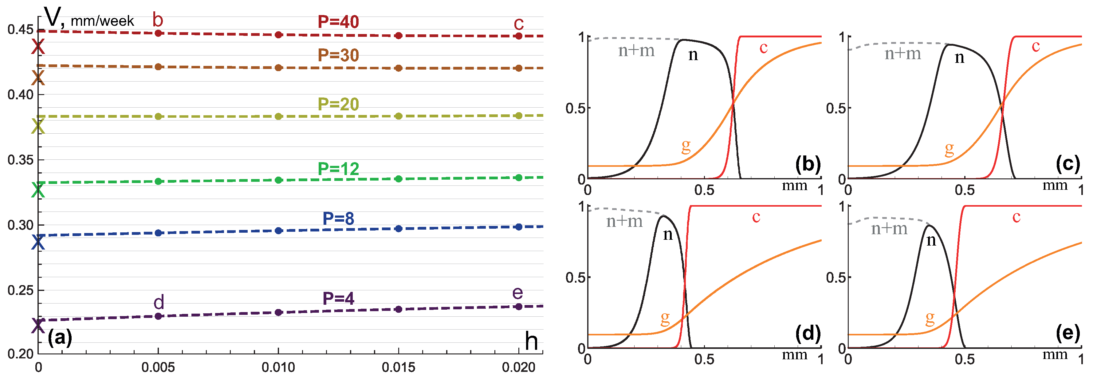
3.2. Invasive Type of Growth

Now, let us obtain an analytical estimation for the growth speed of a solid tumor with non-zero cell motility $D_n$, but neglecting the bulk motion of tissue elements, expressed in Equation (1) by hyperbolic terms. Once again, the solution was sought in the form of a wave, traveling with a constant shape and speed V in an infinite region. The boundary conditions are now modified as:

$$\begin{array}{cccc}\left\{\begin{array}{c}n=0,\\ m=m^{*},\\ g=g^{*},\\ c=0\end{array}\right.\hfill & \hfill forz\to -\infty ;& \left\{\begin{array}{c}n=0,\\ m=0,\\ g=1,\\ c=1\end{array}\right.\hfill & \hfill forz\to +\infty ,\end{array}$$

(8)

where $g^{*}$ and $m^{*}$ are introduced as the limiting constant values of glucose concentration and necrotic tissue fraction at $z\to -\infty$. For the estimation of V, it is necessary to consider the asymptotic behavior of the solutions at $z=\pm \infty$. For this purpose, let us linearize the system (1) at the boundary values (8), neglecting the convective terms, and thus obtain two systems of ODEs with constant coefficients:

$$\{\begin{array}{c}{D}_n{n}_{-}^{″}+V{n}_{-}^{\prime }+B{n}_{-}·[1-\sigma \left(g^{*}\right)]-M{n}_{-}·\sigma \left(g^{*}\right)=0;\hfill \\ V{m}_{-}^{\prime }+M{n}_{-}·\sigma \left(g^{*}\right)=0;\hfill \\ D_g{g}_{-}^{″}+V{g}_{-}^{\prime }+P{c}_{-}[1-g^{*}]-Q{n}_{-}·[1-\sigma (g^{*}\left)\right]=0;\hfill \\ V{c}_{-}^{\prime }-R{m}^{*}{c}_{-}=0.\hfill \end{array}$$

and:

$$\{\begin{array}{c}{D}_n{n}_{+}^{″}+V{n}_{+}^{\prime }+B{n}_{+}·[1-\sigma \left(1\right)]-M{n}_{+}·\sigma \left(1\right)=0;\hfill \\ V{m}_{+}^{\prime }+M{n}_{+}·\sigma \left(1\right)=0;\hfill \\ D_g{g}_{+}^{″}+V{g}_{+}^{\prime }-P{g}_{+}-Q{n}_{+}·[1-\sigma (1\left)\right]=0;\hfill \\ V{c}_{+}^{\prime }-R[n_{+}+m_{+}]=0,\hfill \end{array}$$

where primes denote differentiation with respect to $z=x-Vt$ and subscripts − and + refer to the linearized problems at $z\to -\infty$ and $z\to +\infty$, respectively. The solutions to these problems should be sought in the form ${(n_{\pm }^{\prime },n_{\pm },m_{\pm },g_{\pm }^{\prime },g_{\pm },c_{\pm })}^T\sim {\mathbf{k}}^{\pm }exp\left({\mu }^{\pm }z\right)$, which reduces these systems of linear differential equations to eigenvalue problems.

For $z\to -\infty$, the eigenvalues are:

$$\begin{array}{c}{\mu }_{1,2}^{-}=0,{\mu }_3^{-}=R{m}^{-}/V,{\mu }_4^{-}=-V/D_g,\\ {\mu }_{5,6}^{-}=[-V/2\pm \sqrt{V^2/4+D_n\{M\sigma \left(g^{-}\right)-B[1-\sigma \left(g^{-}\right)]\}}]/D_n,\end{array}$$

where ${\mu }_3^{-}$ is positive, ${\mu }_4^{-}$ is negative, and ${\mu }_{5,6}^{-}$ have opposite signs, since $M\sigma \left(g^{-}\right)-B[1-\sigma \left(g^{-}\right)]>0$, i.e., the death rate exceeds the proliferation rate at sufficiently low values of z, which follows from the physical meaning of the model.

For $z\to +\infty$, the eigenvalues are:

$$\begin{array}{c}{\mu }_{1,2}^{+}=0,{\mu }_{3,4}^{+}=[-V/2\pm \sqrt{V^2/4+D_{g}P}]/D_g,\\ {\mu }_{5,6}^{+}=[-V/2\pm \sqrt{V^2/4-D_n\{B[1-\sigma \left(1\right)]-M\sigma \left(1\right)\}}]/D_n,\end{array}$$

where ${\mu }_{3,4}^{+}$ have opposite signs and, depending on the value of V, ${\mu }_{5,6}^{+}$ are either complex numbers with negative real parts, or real numbers with opposite signs, or both are equal to zero. Therefore, for sufficiently low values of V, the solution may oscillate for large values of z, yielding regions with negative values of n and m, which is physically unrealistic. Thus, the following restriction on tumor growth speed is sufficient for physically reasonable solutions:

$$V\ge V_{min}=2\sqrt{D_n\{B[1-\sigma \left(1\right)]-M\sigma \left(1\right)\}}\approx 2\sqrt{B{D}_n},$$

(9)

the last two values being extremely close under the basic set of parameters, differing by less than ${10}^{-13}\%$ even under a decrease of $ϵ$ up to the value of 20. For the basic set of parameters, $V_{min}\approx 1.063$ mm/week, which was in a good correspondence with the speed of growth of highly invasive tumors [40]. Formula (9) corresponds well to the well-known result regarding Fisher’s equation, which can be written out in the notation used herein as:

$${\displaystyle \frac{\partial n}{\partial t}=Bn(1-n)+D_n\frac{{\partial }^{2}n}{\partial x^2}.}$$

(10)

For this equation, the range of the speed of monotone waves satisfies:

$$V\ge V_{min}^f=2\sqrt{B{D}_n},$$

this result not being affected by the alteration of the proliferation term as long as the proliferation rate tends to B for $n\to 0$. For Fisher’s equation, it is known that if its initial conditions have a compact support, i.e.,

$$n(x,0)=n_0\left(x\right)\ge 0,n_0\left(x\right)=\left\{\begin{array}{c}1ifx\le x_1,\hfill \\ 0ifx\ge x_2,\hfill \end{array}\right.$$

(11)

where $x_1<x_2$ and $n_0\left(x\right)$ is continuous in $x_1<x<x_2$, then the solution $n(x,t)$ of Equation (10) evolves to a traveling wavefront solution with the speed $V_{min}^f=2\sqrt{B{D}_n}$ [47].

The numerical simulations of the system (1) under the neglect of convective terms with the initial conditions (2), which represent a function with a compact support, show that they evolve to the wavefronts, traveling with speeds very close to $2\sqrt{B{D}_n}$. For the basic set of parameters, numerical simulations gave $V\approx 1.061$ mm/week, yielding the same tumor growth speed up to three decimal places (as well as the same number of cells $N\approx 1.383$) under space steps $h=\{0.2,0.1,0.05,0.025\}$ and time steps $\tau =h^2$. Thus, much coarser discretization could provide more accurate results for the considered system under the neglect of convective terms. A dozen simulations under other values of parameters, chosen randomly from the ranges $B\in [0.05,0.3]$ and $D_n\in [0.001,0.4]$, as well produced the values of tumor growth speeds that differed from $2\sqrt{B{D}_n}$ by no more than $0.5\%$.

Since the considered system could be viewed as an augmentation of Fisher’s model, the obtained results suggested that the introduced modifications should not affect the wave speed of its solution, which evolved from a function having a compact support, or at least they should lead to only a very small correction of it within the physiologically justified range of parameters. Most importantly, the parameter P is not present in Formula (9), which implies that angiogenesis should not influence the growth speed of a considered invasive tumor at all. Numerical modeling speaks in favor of this result. The simulations under six values of the angiogenesis parameter within the considered range $P\in [4,40]$ yielded tumor growth speeds equal up to three decimal places, which is illustrated by Figure 4a. The simulations were run with space step $h=0.1$ and time step $\tau =h^2=0.01$, which nevertheless did not allow saving a sufficient amount of computational time, compared to the simulations of Section 3.1, since in this case, the tumor growth speed tended sufficiently slower to a constant value, thus requiring longer simulation on larger domains.

Of note, the number of tumor cells notably grew with the increase of P, as Figure 4a shows, resulting in an ≈72% increase under 10-fold magnification of the basic value of $P=4$. This effect was well noticeable when comparing the profiles of tumor cells under $P=4$ and $P=40$, which are depicted in Figure 4b,c on the 20th day of tumors growth.

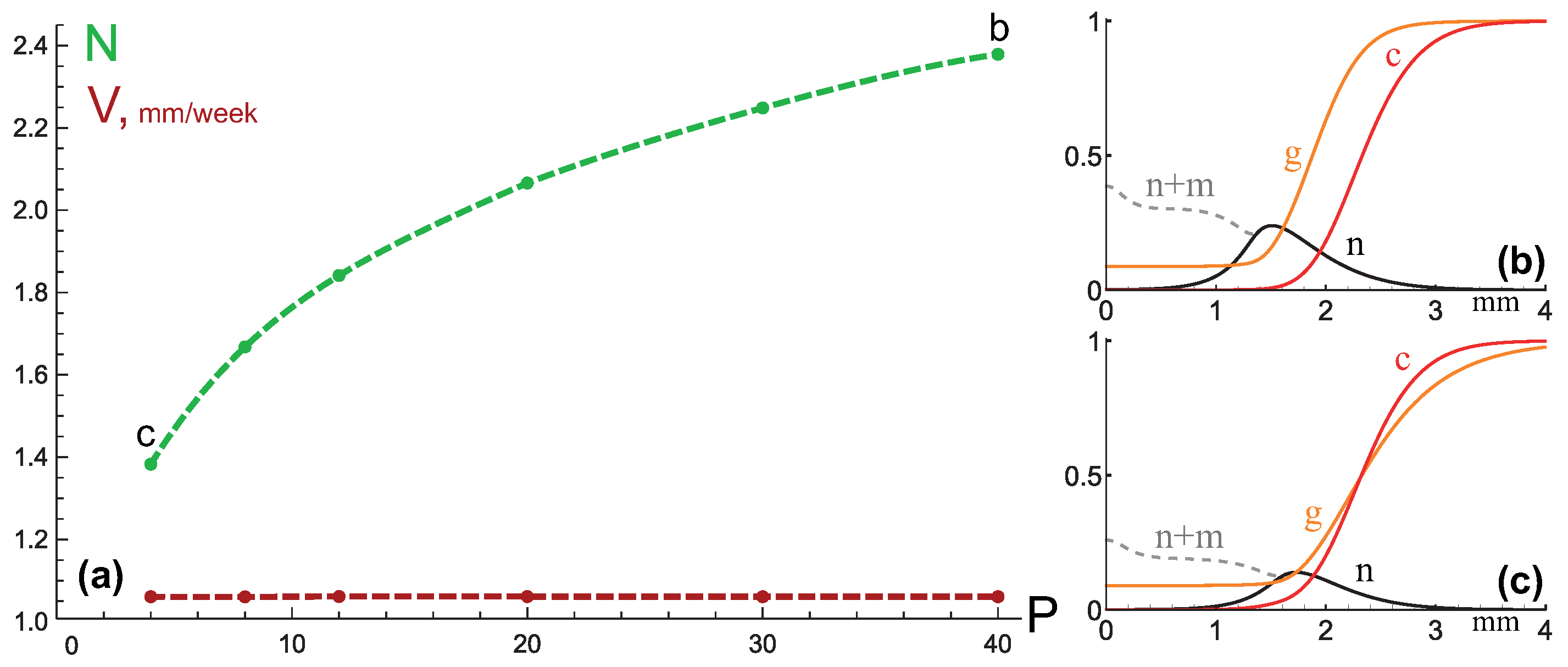
3.3. Mixed Type of Growth

The conclusion of the indifference of invasive tumor growth speed to angiogenesis was valid under the full neglect of the convective component of tumor growth. However, it was reasonable to assume that simultaneously accounting for it should nevertheless lead to a non-zero effect of AAT on the growth speed of an invasive tumor, since the convective component of tumor growth should be affected by the number of its cells. In order to evaluate the effect of antiangiogenic therapy on tumors with a mixed type of growth, the sets of six simulations under different values of angiogenesis parameter P were conducted for eight values of tumor cell motility $D_n$. As a compromise between computing resources and accuracy, the values of space step $h=0.01$ and time step $\tau ={10}^{-4}$ were used. The obtained tumor growth speeds are designated in Figure 5a, where the data for the case with zero cell motility, already shown in Figure 3a, is added.

Let introduce the parameter of “maximum antiangiogenic effect” as:

$${\left(V\right|}_{P=40}{-V|}_{P=4}{)/V|}_{P=40},$$

which indicates how the tumor growth speed would slow down upon a decrease of angiogenesis parameter P from 40 to four, the latter corresponding to the normal microvasculature level. Its dependence on tumor cell motility is shown in Figure 5b, while under $D_n=0$, it was ≈48%. The graph suggests that the effect of mono-AAT should inversely correlate with the invasiveness of the tumor; however, it should be non-zero even for highly invasive tumors, since the maximum antiangiogenic effect, obtained under high values of tumor cell motility, $D_n=0.1$ and $D_n=0.33$, was ≈13% and ≈11%, correspondingly.

An interesting property of the considered tumors with a mixed type of growth was the fact that their growth speed was not equal to the sum of two speeds: $V_{comp}$ that was obtained in the absence of cell motility—i.e., during purely compact growth—and $V_{inv}\approx 2\sqrt{B{D}_n}$ that was obtained in absence of convective flows—i.e., during purely invasive growth. This property is illustrated in Figure 6, which shows the dependence of the parameter $(V-V_{comp})/V_{inv}$ on P for different $D_n$. This parameter may be treated as the ratio of the increase in tumor growth speed, caused by the mobilization of initially immotile cells, to the speed of pure invasive growth itself. The reason for the non-additivity of the growth speeds was the fact that the redistribution of the tumor cells, caused by their migration, led to the change in the number of cells in the proliferating state and altered the convective velocity field. This effect had an ambiguous character. Firstly, the protrusion of tumor cells’ profile towards the region with a normal density of microvasculature led to the increase in the effective rate of capillaries’ degradation, which resulted in a decrease of glucose inflow to the tumor and a subsequent decrease of the pool of proliferating cells. Secondly, this protrusion itself enlarged the pool of tumor cells, located in the region with a concentration of glucose sufficient for their proliferation. The first aspect dominated under small values of $D_n$, leading to a much smaller increase in tumor growth speed, than $2\sqrt{B{D}_n}$. This effect was more pronounced under high values of P, since in this case, tumors had more cells, and therefore enlarged sizes of such protrusions that led to accelerated degradation of capillaries. According to the simulations, a tumor with motile cells may even grow slower than the same tumor with immobilized cells. The second aspect dominated under high values of $D_n$, resulting in the fact that the tumor growth speed was higher than $V_{conv}+V_{dif}$ under $D_n=0.33$ for all the considered values of P.

4. Discussion

The goal of this paper was to study, by means of mathematical modeling, the effect of mono-antiangiogenic therapy (AAT) on monoclonal tumors, which have different types of growth. The analytical estimations performed allowed suggesting that AAT may provide a several times decrease of growth speed for compact tumors, but the decrease of growth speed for invasive tumors should be much less significant. Thus, the tumors, which initially had an invasive phenotype, should possess intrinsic resistance to AAT, while compactly growing tumors should be more susceptible to it. This conclusion corresponds well to the preclinical and clinical data [21,23]. To the best of my knowledge, this effect was not reproduced before via a continuous model of tumor growth, while this ability of the model should be crucial for the investigation of AAT.

The presented model was built on the fundamental principle that the diffusion and consumption of nutrients limit the growth of a solid tumor. This principle underlines a multitude of existing continuous models that account for spatio-temporal interactions between tumor cells and nutrients (see, e.g., [48] for a review). The main distinguishing feature of the presented model was the simultaneous accounting of the intrinsic motility of malignant cells and the convective motion, arising due to their proliferation, which allowed considering two types of tumor growth, as well as their combination. Despite the relative simplicity that this approach has under the assumption of the spherical symmetry of a tumor, it is relatively rarely used, and usually one of the two types of tumor growth is ignored in continuous models. Some of the few exceptions were the work [49], which provided a theoretical justification for the phenomenon of the dominance of a metastatically active population in an avascular heterogeneous tumor, and the work [50], which explained from a theoretical point of view the effect of tumor cells’ migration within a multicellular tumor spheroid. The works [51,52], which also utilized such an approach, were devoted to the investigation of the fingering instability of the avascular tumor surface in the two-dimensional case. This instability could be regarded as a way for a tumor to counteract the diffusional limitations of nutrient inflow. While this phenomenon may affect the tumor growth speed quantitatively, the main qualitative results of the presented work, obtained under the assumption of radial symmetry, could hardly be affected in higher dimensions.

The presented model accounts for glucose as the main nutrient, since it is an indispensable substrate for cell division [28], while most of the relevant models consider tumor cell proliferation to be dependent on oxygen [48]. While such a difference may not be of major importance to the model presented herein, as well as to the models of avascular tumor growth, it should be noted that the approach for modeling the dynamics of oxygen with implicit accounting of tumor vasculature should differ from that for glucose due to the specific features of their blood transport, transvascular transport, and tumor metabolism, which were discussed in the previous paper by our research group [34].

The account of angiogenesis, utilized herein, is rather schematic; however, it allows considering the two major effects of AAT on a qualitative level, allowing performing analytical estimations that suit the purposes of this work. Under more straightforward consideration of angiogenesis, i.e., the introduction of a separate variable for VEGF, which would affect the dynamics of capillaries, one would obtain a distribution of capillaries with non-uniform alterations in their density and permeability [27,34]. However, for every simulation of such an extended model, there will exist a corresponding value of P, which would provide the same increase in tumor growth speed in the simplified model presented herein. Interestingly, the analytical expression for the speed of growth of a compact tumor with no capillaries inside it allowed obtaining a limit of its growth speed under the infinite increase in the number of capillaries and/or in their permeability. However, the estimations with physiologically based values of parameters suggested that achieving more than $\approx 80\%$ of this limit value of speed was unlikely for real tumors. The analytical expression for the speed of growth of invasive tumor indicated that angiogenesis did not influence it at all under the neglect of the convective component of tumor growth, which was confirmed by numerical simulations. However, the simulations, which accounted for both reasons of growth, suggested that in terms of tumor speed reduction, the maximum possible angiogenic effect for highly invasive monoclonal tumors should be around 10–15%.

Importantly, the neglect of convective motion would have led to the misleading conclusion of the indifference of tumor growth speed to angiogenesis for low-invasive tumors as well, since it was not affected by the exact value of tumor cell motility. It should be noted that the accounting of the convective component of tumor growth should be also crucial for modeling of other types of antitumor therapy, since the decrease in the number of tumor cells, caused by any treatment, in reaction-diffusion models should lead to an underestimated decrease of tumor growth speed.

The numerical simulations performed highlighted the non-additive character of the two types of tumor growth. Namely, the addition of a small enough motility to initially immobilized tumor cells should lead to a notably smaller increase in tumor growth speed that could be expected from the analytical estimations of the speed of tumor invasion. Interestingly, the simulations suggested that a low-invasive tumor may even grow slower than the same tumor with immobilized cells. Under sufficiently high cell motility, on the contrary, the two types of tumor growth produced a synergistic effect.

References

1. Sarker, M.S.R.; Pokojovy, M.; Kim, S. On the Performance of Variable Selection and Classification via Rank-Based Classifier. Mathematics 2019, 7, 457. [Google Scholar] [CrossRef] [Green Version]
2. Geng, Y.; Dalhaimer, P.; Cai, S.; Tsai, R.; Tewari, M.; Minko, T.; Discher, D.E. Shape effects of filaments versus spherical particles in flow and drug delivery. Nat. Nanotechnol. 2007, 2, 249. [Google Scholar] [CrossRef] [PubMed]
3. Antico, M.; Prinsen, P.; Cellini, F.; Fracassi, A.; Isola, A.A.; Cobben, D.; Fontanarosa, D. Real-time adaptive planning method for radiotherapy treatment delivery for prostate cancer patients, based on a library of plans accounting for possible anatomy configuration changes. PLoS ONE 2019, 14, e0213002. [Google Scholar] [CrossRef] [PubMed]
4. Boucher, Y.; Baxter, L.; Jain, R. Interstitial pressure gradients in tissue-isolated and subcutaneous tumors: Implications for therapy. Cancer Res. 1990, 50, 4478–4484. [Google Scholar] [PubMed]
5. Gatenby, R.; Gawlinski, E.; Gmitro, A.; Kaylor, B.; Gillies, R. Acid-mediated tumor invasion: A multidisciplinary study. Cancer Res. 2006, 66, 5216–5223. [Google Scholar] [CrossRef] [Green Version]
6. Citron, M.; Berry, D.; Cirrincione, C.; Hudis, C.; Winer, E.; Gradishar, W.; Davidson, N.; Martino, S.; Livingston, R.; Ingle, J.; et al. Randomized trial of dose-dense versus conventionally scheduled and sequential versus concurrent combination chemotherapy as postoperative adjuvant treatment of node-positive primary breast cancer: First report of Intergroup Trial C9741/Cancer and Leukemia Group B Trial 9741. J. Clin. Oncol. 2003, 21, 1431–1439. [Google Scholar]
7. Chmielecki, J.; Foo, J.; Oxnard, G.; Hutchinson, K.; Ohashi, K.; Somwar, R.; Wang, L.; Amato, K.; Arcila, M.; Sos, M.; et al. Optimization of dosing for EGFR-mutant non-small cell lung cancer with evolutionary cancer modeling. Sci. Transl. Med. 2011, 3, 90ra59. [Google Scholar] [CrossRef] [Green Version]
8. Hanahan, D.; Weinberg, R.A. The hallmarks of cancer. Cell 2000, 100, 57–70. [Google Scholar] [CrossRef] [Green Version]
9. Laird, A.K. Dynamics of tumour growth. Br. J. Cancer 1964, 18, 490. [Google Scholar] [CrossRef]
10. Burton, A.C. Rate of growth of solid tumours as a problem of diffusion. Growth 1966, 30, 157–176. [Google Scholar]
11. Rockne, R.; Alvord, E.; Rockhill, J.; Swanson, K. A mathematical model for brain tumor response to radiation therapy. J. Math. Biol. 2009, 58, 561. [Google Scholar] [CrossRef] [PubMed] [Green Version]
12. Alfonso, J.; Köhn-Luque, A.; Stylianopoulos, T.; Feuerhake, F.; Deutsch, A.; Hatzikirou, H. Why one-size-fits-all vaso-modulatory interventions fail to control glioma invasion: In silico insights. Sci. Rep. 2016, 6, 37283. [Google Scholar] [CrossRef] [PubMed]
13. Ward, J.P.; King, J. Mathematical modeling of avascular-tumour growth. Math. Med. Biol. J. IMA 1997, 14, 39–69. [Google Scholar] [CrossRef]
14. Byrne, H.; Drasdo, D. Individual-based and continuum models of growing cell populations: A comparison. J. Math. Biol. 2009, 58, 657. [Google Scholar] [CrossRef]
15. Hahnfeldt, P.; Panigrahy, D.; Folkman, J.; Hlatky, L. Tumor development under angiogenic signaling: A dynamical theory of tumor growth, treatment response, and postvascular dormancy. Cancer Res. 1999, 59, 4770–4775. [Google Scholar]
16. Glick, A.; Mastroberardino, A. An Optimal Control Approach for the Treatment of Solid Tumors with Angiogenesis Inhibitors. Mathematics 2017, 5, 49. [Google Scholar] [CrossRef] [Green Version]
17. Macklin, P.; McDougall, S.; Anderson, A.; Chaplain, M.; Cristini, V.; Lowengrub, J. Multiscale modeling and nonlinear simulation of vascular tumour growth. J. Math. Biol. 2009, 58, 765–798. [Google Scholar] [CrossRef] [Green Version]
18. Kuznetsov, M.; Gorodnova, N.; Simakov, S.; Kolobov, A. Multiscale modeling of angiogenic tumor growth, progression, and therapy. Biophysics 2016, 61, 1042–1051. [Google Scholar] [CrossRef]
19. Vasudev, N.S.; Reynolds, A.R. Anti-angiogenic therapy for cancer: Current progress, unresolved questions and future directions. Angiogenesis 2014, 17, 471–494. [Google Scholar] [CrossRef] [Green Version]
20. Goel, S.; Wong, A.H.K.; Jain, R.K. Vascular normalization as a therapeutic strategy for malignant and nonmalignant disease. Cold Spring Harb. Perspect. Med. 2012, 2, a006486. [Google Scholar] [CrossRef]
21. Ebos, J.M.; Kerbel, R.S. Antiangiogenic therapy: Impact on invasion, disease progression, and metastasis. Nat. Rev. Clin. Oncol. 2011, 8, 210. [Google Scholar] [CrossRef] [PubMed] [Green Version]
22. Ebos, J.M.; Mastri, M.; Lee, C.R.; Tracz, A.; Hudson, J.M.; Attwood, K.; Cruz-Munoz, W.R.; Jedeszko, C.; Burns, P.; Kerbel, R.S. Neoadjuvant antiangiogenic therapy reveals contrasts in primary and metastatic tumor efficacy. EMBO Mol. Med. 2014, 6, 1561–1576. [Google Scholar] [CrossRef] [PubMed]
23. Bergers, G.; Hanahan, D. Modes of resistance to anti-angiogenic therapy. Nat. Rev. Cancer 2008, 8, 592. [Google Scholar] [CrossRef] [PubMed] [Green Version]
24. Pàez-Ribes, M.; Allen, E.; Hudock, J.; Takeda, T.; Okuyama, H.; Viñals, F.; Inoue, M.; Bergers, G.; Hanahan, D.; Casanovas, O. Antiangiogenic therapy elicits malignant progression of tumors to increased local invasion and distant metastasis. Cancer Cell 2009, 15, 220–231. [Google Scholar] [CrossRef] [Green Version]
25. Kolobov, A.; Kuznetsov, M. Investigation of the effects of angiogenesis on tumor growth using a mathematical model. Biophysics 2015, 60, 449–456. [Google Scholar] [CrossRef]
26. Kuznetsov, M.B.; Kolobov, A.V. Mathematical investigation of antiangiogenic monotherapy effect on heterogeneous tumor progression. Comput. Res. Model. 2017, 9, 487–501. [Google Scholar] [CrossRef] [Green Version]
27. Kuznetsov, M.B.; Gubernov, V.V.; Kolobov, A.V. Analysis of anticancer efficiency of combined fractionated radiotherapy and antiangiogenic therapy via mathematical modeling. Russ. J. Numer. Anal. Math. Model. 2018, 33, 225–242. [Google Scholar] [CrossRef]
28. Patra, K.C.; Hay, N. The pentose phosphate pathway and cancer. Trends Biochem. Sci. 2014, 39, 347–354. [Google Scholar] [CrossRef] [Green Version]
29. Levick, J.R. An Introduction to Cardiovascular Physiology; Butterworth-Heinemann: Oxford, UK, 2013. [Google Scholar]
30. Araujo, R.; McElwain, D. New insights into vascular collapse and growth dynamics in solid tumors. J. Theor. Biol. 2004, 228, 335–346. [Google Scholar] [CrossRef]
31. Holash, J.; Maisonpierre, P.; Compton, D.; Boland, P.; Alexander, C.; Zagzag, D.; Yancopoulos, G.; Wiegand, S. Vessel cooption, regression, and growth in tumors mediated by angiopoietins and VEGF. Science 1999, 284, 1994–1998. [Google Scholar] [CrossRef] [Green Version]
32. Swanson, K.R.; Rockne, R.C.; Claridge, J.; Chaplain, M.A.; Alvord, E.C.; Anderson, A.R. Quantifying the role of angiogenesis in malignant progression of gliomas: In silico modeling integrates imaging and histology. Cancer Res. 2011, 71, 7366–7375. [Google Scholar] [CrossRef] [PubMed] [Green Version]
33. Szomolay, B.; Eubank, T.D.; Roberts, R.D.; Marsh, C.B.; Friedman, A. Modeling the inhibition of breast cancer growth by GM-CSF. J. Theor. Biol. 2012, 303, 141–151. [Google Scholar] [CrossRef] [PubMed]
34. Kuznetsov, M.; Kolobov, A. Transient alleviation of tumor hypoxia during first days of antiangiogenic therapy as a result of therapy-induced alterations in nutrient supply and tumor metabolism—Analysis by mathematical modeling. J. Theor. Biol. 2018, 451, 86–100. [Google Scholar] [CrossRef] [PubMed]
35. Maeda, H.; Wu, J.; Sawa, T.; Matsumura, Y.; Hori, K. Tumor vascular permeability and the EPR effect in macromolecular therapeutics: A review. J. Control. Release 2000, 65, 271–284. [Google Scholar] [CrossRef]
36. Fu, B.M.; Shen, S. Structural mechanisms of acute VEGF effect on microvessel permeability. Am. J. Physiol.-Heart Circ. Physiol. 2003, 284, H2124–H2135. [Google Scholar] [CrossRef] [PubMed] [Green Version]
37. Abdollahi, A.; Lipson, K.E.; Sckell, A.; Zieher, H.; Klenke, F.; Poerschke, D.; Roth, A.; Han, X.; Krix, M.; Bischof, M.; et al. Combined therapy with direct and indirect angiogenesis inhibition results in enhanced antiangiogenic and antitumor effects. Cancer Res. 2003, 63, 8890–8898. [Google Scholar] [PubMed]
38. Dings, R.P.; Loren, M.; Heun, H.; McNiel, E.; Griffioen, A.W.; Mayo, K.H.; Griffin, R.J. Scheduling of radiation with angiogenesis inhibitors anginex and Avastin improves therapeutic outcome via vessel normalization. Clin. Cancer Res. 2007, 13, 3395–3402. [Google Scholar] [CrossRef] [Green Version]
39. Freyer, J.; Sutherland, R. A reduction in the in situ rates of oxygen and glucose consumption of cells in EMT6/Ro spheroids during growth. J. Cell. Physiol. 1985, 124, 516–524. [Google Scholar] [CrossRef]
40. Swanson, K.; Alvord, E., Jr.; Murray, J. A quantitative model for differential motility of gliomas in grey and white matter. Cell Proliferat. 2000, 33, 317–329. [Google Scholar] [CrossRef]
41. Stamatelos, S.; Kim, E.; Pathak, A.; Popel, A. A bioimage informatics based reconstruction of breast tumor microvasculature with computational blood flow predictions. Microvasc. Res. 2014, 91, 8–21. [Google Scholar] [CrossRef] [Green Version]
42. Tuchin, V.; Bashkatov, A.; Genina, E.; Sinichkin, Y.; Lakodina, N. In vivo investigation of the immersion-liquid-induced human skin clearing dynamics. Tech. Phys. Lett. 2001, 27, 489–490. [Google Scholar] [CrossRef]
43. Dickson, P.V.; Hamner, J.B.; Sims, T.L.; Fraga, C.H.; Ng, C.Y.; Rajasekeran, S.; Hagedorn, N.L.; McCarville, M.B.; Stewart, C.F.; Davidoff, A.M. Bevacizumab-induced transient remodeling of the vasculature in neuroblastoma xenografts results in improved delivery and efficacy of systemically administered chemotherapy. Clin. Cancer Res. 2007, 13, 3942–3950. [Google Scholar] [CrossRef] [PubMed] [Green Version]
44. Boris, J.P.; Book, D.L. Flux-corrected transport. I. SHASTA, a fluid transport algorithm that works. J. Comput. Phys. 1973, 11, 38–69. [Google Scholar] [CrossRef]
45. Press, W.H.; Teukolsky, S.A.; Vetterling, W.T.; Flannery, B.P. Numerical Recipes 3rd Edition: The Art of Scientific Computing; Cambridge University Press: Cambridge, UK, 2007. [Google Scholar]
46. Tamaskar, I.; Garcia, J.A.; Elson, P.; Wood, L.; Mekhail, T.; Dreicer, R.; Rini, B.I.; Bukowski, R.M. Antitumor effects of sunitinib or sorafenib in patients with metastatic renal cell carcinoma who received prior antiangiogenic therapy. J. Urol. 2008, 179, 81–86. [Google Scholar] [CrossRef]
47. Kolmogorov, A.N. Étude de l’équation de la diffusion avec croissance de la quantité de matière et son application à un problème biologique. Bull. Univ. Moskow Ser. Intern. Sect. A 1937, 1, 1–25. [Google Scholar]
48. Roose, T.; Chapman, S.J.; Maini, P.K. Mathematical models of avascular tumor growth. SIAM Rev. 2007, 49, 179–208. [Google Scholar] [CrossRef] [Green Version]
49. Kolobov, A.; Polezhaev, A.; Solyanik, G. The role of cell motility in metastatic cell dominance phenomenon: Analysis by a mathematical model. Comput. Math. Methods Med. 2000, 3, 63–77. [Google Scholar] [CrossRef] [Green Version]
50. Thompson, K.; Byrne, H. Modelling the internalization of labelled cells in tumour spheroids. Bull. Math. Biol. 1999, 61, 601–623. [Google Scholar] [CrossRef]
51. Franks, S.; King, J. Interactions between a uniformly proliferating tumour and its surroundings: Uniform material properties. Math. Med. Biol. 2003, 20, 47–89. [Google Scholar] [CrossRef]
52. Franks, S.; King, J. Interactions between a uniformly proliferating tumour and its surroundings: Stability analysis for variable material properties. Int. J. Eng. Sci. 2009, 47, 1182–1192. [Google Scholar] [CrossRef]
Figure 1. The form of the solution of Equation (5), which is searched for analytically.
Mathematics 08 00760 g001
Figure 2. (a) The dots denote the values of tumor growth speed V, obtained numerically in the simulations of Equation (1) under designated values of angiogenesis parameter P and space step h, with time step τ = h 2 , D n = 0 , R = M = 0.1 / τ , ϵ = 10 5 and the values of other parameters taken from the basic set. The dashed lines represent the best fit quadratic functions for every value of P. The crosses on the vertical axis mark the analytically derived values of tumor growth speed for the values of P used. (be) The distributions of the model variables on the 20th day of simulations under the values of the parameters, designated by the corresponding letters in (a).
Mathematics 08 00760 g002
Figure 3. (a) The dots denote the values of tumor growth speed V, obtained numerically in the simulations of Equation (1) under designated values of angiogenesis parameter P and space step h, with time step τ = h 2 , D n = 0 , and the values of other parameters taken from the basic set. The dashed lines represent the best fit quadratic functions for every value of P. The crosses on the vertical axis mark the analytically derived values of tumor growth speed for the values of P used. (be) The distributions of the model variables on the 20th day of simulations under the values of the parameters, designated by the corresponding letters in (a).
Mathematics 08 00760 g003
Figure 4. (a) The red dots denote the values of tumor growth speed V; the green dots denote the values of number of tumor cells N, which were obtained numerically in the simulations of Equation (1) with the neglect of hyperbolic terms (i.e., I = 0 ) under designated values of angiogenesis parameter P, values of other parameters, taken from the basic set, space step h = 0.1 , and time step τ = 0.01 . The dashed lines are interpolations of data points. (b,c) The distributions of the model variables on the 20th day of simulations under P = 40 and P = 4 correspondingly.
Mathematics 08 00760 g004
Figure 5. (a) The dots denote the values of tumor growth speeds V, obtained numerically in the simulations of Equation (1) with space step h = 0.01 and time step τ = 10 4 , under designated values of angiogenesis parameter P and tumor cell motility D n and the values of other parameters taken from the basic set. The dashed lines are interpolations of data points. (b) The graph of “maximum angiogenic effect”, based on the data, shown in (a), which shows how the tumor growth speed would slow down upon the decrease of angiogenesis parameter P from 40 to four under designated values of D n .
Mathematics 08 00760 g005
Figure 6. The dots denote the ratios of the differences of tumor growth speed V and V c o m p , which is the growth speed of the same tumor under zero cell motility, to V i n v , which is the growth speed of the same tumor under the neglect of convective flows. All values were obtained numerically in the simulations of Equation (1) with space step h = 0.01 and time step τ = 10 4 under designated values of angiogenesis parameter P and tumor cell motility D n and the values of other parameters taken from the basic set. The dashed lines are interpolations of data points.
Mathematics 08 00760 g006