A Hidden Markov Model to Address Measurement Errors in Ordinal Response Scale and Non-Decreasing Process

Abstract

A Bayesian approach was developed, tested, and applied to model ordinal response data in monotone non-decreasing processes with measurement errors. An inhomogeneous hidden Markov model with continuous state-space was considered to incorporate measurement errors in the categorical response at the same time that the non-decreasing patterns were kept. The computational difficulties were avoided by including latent variables that allowed implementing an efficient Markov chain Monte Carlo method. A simulation-based analysis was carried out to validate the approach, whereas the proposed approach was applied to analyze aortic aneurysm progression data.

1. Introduction

Statistical modeling depends on accurate data to provide reliable results in many contexts. This is especially relevant in the case of medical diagnosis. Since the human factor is introduced in the data collection processes, errors may occur. For example, when modeling a degenerative disease, which should produce non-decreasing outcome data over time, it may happen that some data do not satisfy this condition, mainly due to human factors. Therefore, additional parameters should be included in the statistical approach to correct the bias yielded by the use of error-prone data. Ignoring measurement errors may lead, in many cases, to non-optimal decisions (see, e.g., [1,2]). For example, the wrong estimations can be obtained for the sensitivity and specificity of diagnostic tests, which may lead to errors in positive and negative predictive values, implying diagnostic errors. Thus, statistical models should incorporate correction mechanisms for measurement errors to produce proper inference.

In the scientific literature, there are different approaches considering measurement errors in different contexts, depending on the type of observed data. When a measurement error occurs in a categorical variable, it is called misclassification. The work in [3] proposed statistical models for phenomena with misclassified ordinal responses in the multivariate case. The work in [4] considered covariates with missing data. The work in [5] addressed misclassified ordinal response data based on a cross-sectional framework. For misclassified longitudinal data with categorical responses, The works in [6,7] considered generalized linear mixed models, whereas [6,8,9] used approaches based on generalized estimating equations.

Multi-state transitional models and hidden Markov models (HMM) are useful for quantifying disease staging. They can be used to examine measurement error and misclassification in longitudinal studies where the outcome is continuous or categorical in both continuous and discrete time settings. For binary misclassifications with non-monotone longitudinal responses, HMM have been considered by several authors ( e.g., [10,11]). The works in [12,13,14,15] addressed the problem of misclassified monotone longitudinal responses. The work in [16,17,18] proposed models for longitudinal data with ordinal responses subject to misclassification in a non-continuous internal process.

HMM with random effects [19], also called mixed hidden Markov models (MHMM), have been used to cope with misclassification in multilevel data [20] and longitudinal data [21]. The model parameters of HMM and MHMM for true monotone responses may be estimated without the use of external information on the misclassification parameters. Recently, the works in [22,23] developed approaches based on HMM to model measurement errors in continuous and binary responses, respectively, in the context of non-decreasing processes. In this paper, an HMM is proposed to address measurement errors in the ordinal response in the context of monotone non-decreasing processes. A Bayesian framework is presented with an efficient Markov chain Monte Carlo (MCMC) method that solves the computational problem. The approach is applied to simulated data in order to evaluate its performance and to the problem of grading aortic aneurysms based on misclassified data.

In the proposed approach, the true process by which the disease develops can be modeled continuously, but this level of measurement is transformed into an ordinal scale for practical purposes. Furthermore, considering that the process is non-decreasing, it is assumed that the disease progressively worsens. Aortic aneurysm is an example of the type of disease that can be modeled with this approach, since it is a located and permanent dilation that occurs in the aorta and is caused by a progressive degeneration of its wall. It must be monitored because its natural evolution is growth until breakage. Its diagnosis is based on the diameter of the aorta [24], but it is staged by severity, according to successive ranges of aortic diameter in an ordinal scale (from Stages 1 to 4). Besides, this disease is prone to measurement errors due to the ultrasound equipment and/or its management.

The rest of the paper is organized as follows. Section 2 includes the proposed approach considering non-decreasing time processes with measurement error in the ordinal response and the conditional independence assumptions. In Section 3, a Bayesian analysis is presented. Section 4 shows the model performance with a simulation-based example, whereas the analysis of the aortic aneurysm data is presented in Section 5. Finally, the conclusions are presented in Section 6.

2. The Model

The proposed approach considered a time-dependent process, which was continuous and monotone non-decreasing. It addressed the measurement errors in the ordinal response, and it took into account several conditional independence assumptions. The following subsections describe the approach.

2.1. A Continuous Monotone Non-Decreasing Process

N response scores were considered, all of them recorded at time points $t_{i{k}_i}$, $i=1,\dots ,N$ and $k_i=1,\dots ,K_i.$ Without loss of generality and for the sake of simplicity, the subjects were assumed to have the same number of time points, which is denoted by $K.$ Nevertheless, this is only a notation issue, and a different number of time points could be handled by the approach. Let $W_{ik}$ be the true response for the ith subject at time $t_{ik},$ such as $W_{i1}\le W_{i2}\le \cdots \le W_{i,K-1}\le W_{iK},$ for all i. This means that $\left\{W_{ik}\right\}$ is a monotone non-decreasing continuous process, representing the true gradual process, which is difficult to score quantitatively, and it is not observable. Therefore, let $\left\{Y_{ik}^{*}\right\}$ be a process that is recorded and subject to measurement error, which will be introduced in Section 2.2.

Now, consider two vectors of covariates associated with the ith subject: ${\mathit{x}}_i,$ which is a non time-varying L-dimensional vector, and ${\mathit{z}}_{ik},$ which is a time-varying M-dimensional vector at time point $t_{ik}$. Moreover, ${\mathit{z}}_i={({\mathit{z}}_{i1},\dots ,{\mathit{z}}_{iK})}^{\prime }$ represents the vector of covariates for the ith subject. Let ${\eta }_{ik}$ be the linear predictors for the ith subject at time $t_{ik}$, consisting of linear combinations of the covariates ${\mathit{x}}_i$ and ${\mathit{z}}_{ik},$ i.e.:

$$\begin{array}{ccc}\hfill {\eta }_{ik}& =& {\mathit{x}}_i^{\prime }\mathit{\beta }+{\mathit{z}}_{ik}^{\prime }\mathit{\gamma },\hfill \end{array}$$

(1)

where $\mathit{\beta }$ and $\mathit{\gamma }$ are the L-dimensional and M-dimensional vectors of coefficients for the covariates ${\mathit{x}}_i$ and ${\mathit{z}}_{ik},$ respectively. Then, ${\mathit{W}}_i={(W_{i1},\dots ,W_{iK})}^{\prime }$ is the unknown response vector that is related to a set of the exogenous covariates ${\mathit{x}}_i$ and ${\mathit{z}}_{ik}$ through the following equations (see [22]):

$$\begin{array}{ccc}\hfill W_{i1}& \sim & \mathrm{N}\left({\eta }_{i1},1\right)\hfill \end{array}$$

(2)

$$\begin{array}{ccc}\hfill W_{ik}|W_{i,k-1}=w_{i,k-1}& \sim & \mathrm{N}\left({\eta }_{ik},1\right)\mathrm{I}\left[W_{ik}\ge w_{i,k-1}\right],k=2,\dots ,K,\hfill \end{array}$$

(3)

where $\mathrm{I}[·]$ denotes the indicator function. Since the $W_{ik}$’s are unobserved and in order to avoid identifiability problems, the variances of the normal distributions were set to one. Moreover, a first-order Markov chain property for continuous processes was assumed, and the truncation allowed the non-decreasing restriction to be satisfied.

2.2. Addressing Measurement Errors in Ordinal Response

The response variables $W_{ik}$ are latent variables assumed to be prone to measurement errors. Let $Y_{ik}^{*}$ be the non-error-free ordinal response for subject i at time $t_{ik},$ where $Y_{ik}^{*}$ takes one of J categories. Thus, ${\mathit{Y}}_i^{*}={(Y_{i1}^{*},\dots ,Y_{iK}^{*})}^{\prime }$ denotes the observed score, which may have been measured with error, and with either non-decreasing or decreasing patterns.

Let $p_{ikj}=\mathbb{P}[Y_{ik}^{*}=j|{\mathit{x}}_i,{\mathit{z}}_{ik}]$ denote the probability that the ith subject at time $t_{ik}$ is classified in the jth category for $j=1,\dots ,J.$ For ordered response categories, the ordinal model can be defined by cutpoints ${\kappa }_0,{\kappa }_1,\dots ,{\kappa }_{J-1},{\kappa }_J,$ considering that $p_{ikj}=\mathsf{\Psi }\left({\kappa }_j-{\eta }_{ik}\right)-\mathsf{\Psi }\left({\kappa }_{j-1}-{\eta }_{ik}\right),$ where $\mathsf{\Psi }(·)$ is a cumulative distribution function (cdf) (see [25]). Let $\mathit{\kappa }={\left({\kappa }_1,\dots ,{\kappa }_{J-1}\right)}^{\prime }$ be the vector of unknown cutpoints with ${\kappa }_0=-\infty$ and ${\kappa }_J=\infty .$ In order to avoid parameter identifiability problems, the intercept term is excluded from the linear predictor ${\eta }_{ik}$, or it is included, but with only $J-2$ unknown cutpoints $\mathit{\kappa }=({\kappa }_2,\dots ,{\kappa }_{J-1})$ where ${\kappa }_1=0$.

Now, based on the data augmentation framework for the ordinal regression model proposed by [25,26], let $W_{ik}^{*}$ be the non error-free continuous response for subject i at time $t_{ik}$ having $\mathsf{\Psi }$ as the cdf. These variables $W_{ik}^{*}$ are related to $Y_{ik}^{*}$ by:

$$\begin{array}{ccc}\hfill Y_{ik}^{*}=j& \mathrm{if}& {\kappa }_{j-1}<W_{ik}^{*}\le {\kappa }_j,\mathrm{for}j=1,\dots ,J.\hfill \end{array}$$

(4)

Measurement error is here assumed to occur on the latent continuous variable $W_{ik}^{*}$, which has a normal distribution conditional on $W_{ik}$ (see [1] and [2]), i.e.:

$$\begin{array}{ccc}\hfill W_{ik}^{*}|W_{ik}=w_{ik}& \sim & \mathrm{N}(w_{ik},{\sigma }^2).\hfill \end{array}$$

(5)

Note that in the case that there is information about who examined each subject i at each time $k,$ then a different variance parameter could be used to estimate the degree of error made by each examiner. Moreover, different cutpoints could be considered for each time point.

2.3. Conditional Independence Assumptions

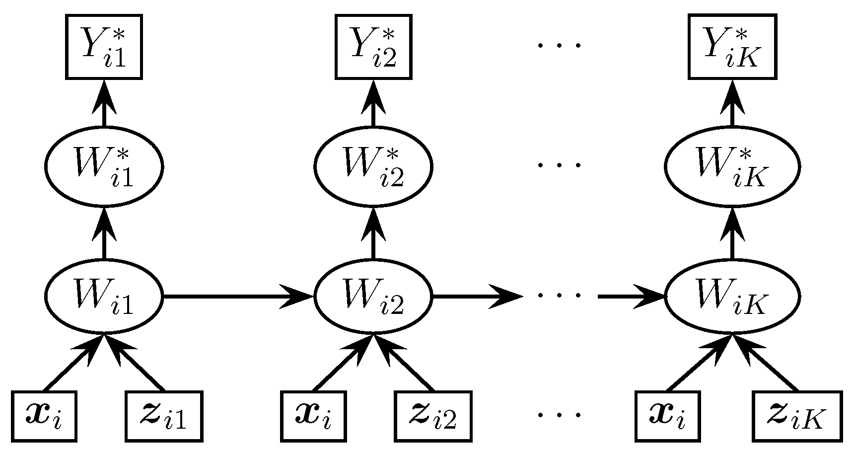
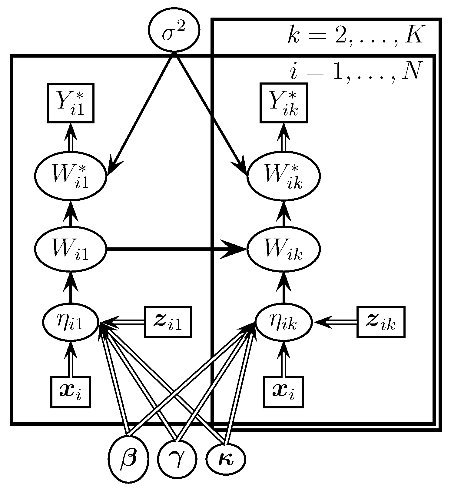
The proposed full model is an inhomogeneous hidden Markov model with a continuous state-space that is comprised of Equations (1)–(5). Figure 1 displays the probabilistic graphical representation showing the dependencies among the variables in the proposed model. The usual convention of graphical models is followed.

The process is characterized by the following conditional independence assumptions (see also [27]):

• ${⫫}_{1\le i\le N}{\mathit{Y}}_i^{*}|{\mathit{W}}_1,\dots ,{\mathit{W}}_N,{\sigma }^2,$ i.e., the observed ordinal response vectors for each subject are independent given the true unobserved continuous responses and the variance of the measurement error.
• ${\mathit{Y}}_i^{*}⫫{\mathit{W}}_1,\dots ,{\mathit{W}}_{i-1},{\mathit{W}}_{i+1},\dots ,{\mathit{W}}_N|{\mathit{W}}_i,{\sigma }^2$, $\forall i,$ i.e., the distribution of the observed ordinal response vector for a subject only depends on his/her true unobserved continuous response vector and the variance of the measurement error.
• ${⫫}_{1\le k\le K}{Y}_{ik}^{*}|{\mathit{W}}_i,{\sigma }^2,$$\forall (i,k),$ i.e., the observed ordinal response for a subject at one time point is independent of the one for the same subject at any other point of time, given the subject’s true unobserved continuous response vector and the measurement error variance.
• $Y_{ik}^{*}⫫W_{i1},\dots ,W_{i,k-1},W_{i,k+1},\dots ,W_{iK}|W_{ik},{\sigma }^2,$ i.e., the distribution of the observed ordinal response in the kth examination only depends on the subject’s true unobserved continuous response at the same examination and variance of the measurement error.

These conditional independence assumptions lead to distributions that are free of other model parameters. In particular, they are independent of parameters $\mathit{\beta },$ $\mathit{\gamma }$, and $\mathit{\kappa },$ and they are also independent of the observed variables $\mathit{x}$ and $\mathit{z}.$ Note that these assumptions are a natural extension of the usual conditional independence assumptions of the HMM proposed by [28].

3. Bayesian Analysis

In this section, the Bayesian analysis is presented, including the MCMC algorithm used.

3.1. The Prior Distributions

Some components of the prior distribution were chosen to be conditionally conjugate distributions. For the coefficients of the covariates in the linear predictor, normal distributions were considered, i.e., $\mathit{\beta }\sim {\mathrm{N}}_L(\mathit{b},\mathit{B})$ and $\mathit{\gamma }\sim {\mathrm{N}}_M(\mathit{c},\mathit{C}).$ The inverse Gamma (IG) was taken for the prior distribution of the variance parameter related to the measurement error model, namely ${\sigma }^2\sim \mathrm{IG}(s,r).$ For the cutpoints $\mathit{\kappa }$, a flat prior distribution was used, i.e., $\pi \left(\mathit{\kappa }\right)\propto 1.$ Note that all these distributions allow obtaining the posterior distributions in an easy way.

3.2. Exploring the Posterior Distribution

Based on the independence assumptions defined in Section 2.3, the likelihood function has the following form:

$$\begin{array}{c}{\displaystyle \mathcal{L}\left({\mathit{W}}^{*},\mathit{W},\mathit{\beta },\mathit{\gamma },\mathit{\kappa },{\sigma }^2|{\mathit{Y}}^{*},\mathit{x},\mathit{z}\right)}\hfill \\ =\prod _{i=1}^N\left\{\left[\prod _{k=1}^K\mathrm{P}\left(Y_{ik}^{*}|W_{ik}^{*},\mathit{\kappa }\right)\mathrm{P}\left(W_{ik}^{*}|W_{ik},{\sigma }^2\right)\right]\right.\hfill \\ \times \mathrm{P}\left(W_{i1}|{\mathit{x}}_i,{\mathit{z}}_{i1},\mathit{\beta },\mathit{\gamma }\right)\left.\left[\prod _{k=2}^K\mathrm{P}\left(W_{ik}|W_{i,k-1},{\mathit{x}}_i,{\mathit{z}}_{ik},\mathit{\beta },\mathit{\gamma }\right)\right]\right\}.\hfill \end{array}$$

(6)

Therefore, from (6) and the prior distributions, the joint posterior distribution is given by:

$$\begin{array}{c}{\displaystyle \pi \left({\mathit{W}}^{*},\mathit{W},\mathit{\beta },\mathit{\gamma },\mathit{\kappa },{\sigma }^2|{\mathit{Y}}^{*},\mathit{x},\mathit{z}\right)}\hfill \\ \propto \mathcal{L}\left({\mathit{W}}^{*},\mathit{W},\mathit{\beta },\mathit{\gamma },\mathit{\kappa },{\sigma }^2|{\mathit{Y}}^{*},\mathit{x},\mathit{z}\right)\pi \left(\mathit{\beta }\right)\pi \left(\mathit{\gamma }\right)\pi \left(\mathit{\kappa }\right)\pi \left({\sigma }^2\right).\hfill \end{array}$$

(7)

Note that the posterior inference considers the relationship between the covariates and the latent variables jointly with the prior distributions. Figure 2 shows a graphical representation of the proposed model. This is based on the doodle objects of WinBUGS [29]. It represents a direct acyclic graph, where the nodes are the model variables and the arrows show dependencies between them. There are two rectangular frames representing sets of identical repeating operations. One panel is indexed by i and ranges from one to N (subjects), and the second panel is indexed by k and ranges from two to K (time points). The variables $Y_{ik}^{*},$ and ${\mathit{x}}_i$, and ${\mathit{z}}_{ik}$ are represented by rectangular boxes, and they correspond to the response variables subject to measurement error and the exactly known independent variables, respectively. The stochastic variables $W_{ik}^{*}$ and $W_{ik}$ (latent variables related to the responses) are represented by oval nodes with the heads of the simple arrows pointing to them. The linear predictors ${\eta }_{ik}$ depend on the variables and parameters from which their arrows start, and these are represented by double-lined arrows pointing to them. Finally, the parameters $\mathit{\beta },$$\mathit{\gamma },$ $\mathit{\kappa }$, and ${\sigma }^2$ are stochastic, with distributions depending on other hyperparameters.

Since (7) is not directly tractable for computing, a Markov chain Monte Carlo method was used [30]. The proposed approach was implemented in JAGS software (http://mcmc-jags.sourceforge.net/) through the R platform (https://cran.r-project.org/). Source codes and instructions can be downloaded from the GitHub repository through the link https://github.com/lizbethna/HMMprogressionOrdinal.git.

4. Simulation Example

A procedure was implemented to generate one hundred datasets. A set of measurements for $N=100$ subjects at $K=6$ time points was simulated. The covariates ${\mathit{x}}_i$ and ${\mathit{z}}_{ik}$ were generated from uniform distributions, $x_{il}\sim \mathrm{U}(0,1)$ and $z_{ikm}\sim \mathrm{U}(0,1),$ for $i=1,\dots ,N,$ $k=1,\dots ,K,$ $l=1,\dots ,L$, and $m=1,\dots ,M,$ and they were vectors of dimension $L=2$ and $M=2,$ respectively, for subject i at time point $k.$ Linear predictors of Equation (1) were computed by using $\mathit{\beta }={(-1,1)}^{\prime }$ and $\mathit{\gamma }={(-1,1)}^{\prime }.$

The true responses $w_{ik}$ were generated by Equations (2) and (3). Now, considering the conditional independence assumptions and $J=4$ categories, the responses subject to measurement error $Y_{ik}^{*}$ were generated by Equation (4), by using the cutpoints $\mathit{\kappa }=(0,2,4)$, and two values for the standard deviation parameter of the measurement error were considered, assuming two different values for the measurement errors that were committed, ${\sigma }_1=0.5$ (for the first half of the subjects) and ${\sigma }_2=1$ (for the other subjects), defined by the latent continuous variable subject to measurement error $w_{ik}^{*}$ in (5).

Using the simulation-based procedure previously described, one-hundred datasets with 100 subjects each were generated.

Table 1. Simulated data: rates of transitions between states.

		States at time ${\mathit{t}}_{\mathit{i},\mathit{k}+1}$
		State 1	State 2	State 3	State 4
States	State 1	0.05402	0.10328	0.02266	0.00092
at	State 2	0.02776	0.25406	0.16908	0.01118
time	State 3	0.00302	0.06454	0.21316	0.03912
$t_{ik}$	State 4	0.00006	0.00300	0.01928	0.01486

shows the average transition rates between stages.

In order to assess the model generalization performance, a cross-validation was considered, splitting datasets into training (75% of the subjects) and testing subsets. Using the training data, the model parameters were estimated, and using the testing data, the classification errors were computed. This was performed for all simulated datasets, and then, the results were averaged.

For the prior distributions, the following were considered: $\mathit{\beta }\sim {\mathrm{N}}_L(\mathbf{0},\mathrm{diag}\left(10,000\right)),$ $\mathit{\gamma }\sim {\mathrm{N}}_M(\mathbf{0},\mathrm{diag}\left(10,000\right)),$ and ${\sigma }^2\sim \mathrm{IG}(0.001,0.001).$ Now, in order to obtain the convergence of the MCMC algorithm, twenty-thousand iterations were considered, with a burn-in of 5000. For each chain, a thinning period of 10 generated values was considered, resulting in a reduced chain of length 2000. The convergence analysis was performed by using the BOA package [31].

After applying the MCMC algorithm with the previous specifications, the posterior distribution was estimated.

Table 2. Simulated data: means and standard deviations (SD) of the posterior estimates of the model parameters based on the 100 generated datasets.

Parameter	True	Mean	SD
${\beta }_1$	$-1$	−0.99178	0.30584
${\beta }_2$	1	1.07347	0.33454
${\gamma }_1$	$-1$	−0.98747	0.37299
${\gamma }_2$	1	0.96573	0.31908
${\kappa }_1$	0	0	—
${\kappa }_2$	2	2.03908	0.13337
${\kappa }_3$	4	4.11077	0.22114
${\sigma }_1$	$0.5$	0.51851	0.07393
${\sigma }_2$	$1.0$	1.03625	0.10296

presents the means and standard deviations of the posterior estimates of the regression coefficients and variance parameters based on the 100 generated datasets.

Note that the estimation of the parameters was reasonably well recovered, showing small biases. Moreover, models with measurement errors usually required external information on the parameters to correct the error, which could be given via informative prior distributions. The proposed vague informative prior distributions provided good results, since the model managed to capture the measurement errors of the response variable properly.

In order to measure the goodness-of-fit of the approach, the mean absolute error (MAE) and root mean squared error (RMSE) were considered.

Table 3. Simulated data: means and standard deviations (between brackets) of two goodness-of-fit criteria for the approach based on the 100 generated datasets.

	Criteria$({\mathit{w}}^{*},\widehat{\mathit{w}})$
	Training	Testing
MAE	1.19077 (0.06181)	1.19914 (0.05929)
RMSE	1.38327 (0.06539)	1.39308 (0.06577)
	Criteria$(\mathit{w},\widehat{\mathit{w}})$
	Training	Testing
MAE	1.01441 (0.06107)	1.02015 (0.05341)
RMSE	1.13663 (0.06290)	1.14334 (0.05261)

shows the means and the standard deviations (between brackets) of the goodness-of-fit criteria obtained with the specified cross-validation scheme. The results showed greater errors between the observed responses and the estimated ones (${\mathit{W}}^{*}$,$\widehat{\mathit{W}}$) than those between the non-decreasing generated responses and the estimated values ($\mathit{W}$,$\widehat{\mathit{W}}$).

Note that the parameters of the model could be estimated without using external information about the measurement error parameters, i.e., the approach was able to obtain information from data in order to estimate the parameters related to measurement errors.

5. Aortic Aneurysm Progression

An aortic aneurysm is an abnormal bulge that occurs in the wall of the aorta, which is greater than 1.5 times its normal size [24]. Aortic aneurysms can occur anywhere in the aorta and may be tube-shaped or rounded. If an aneurysm grows large, it can burst and cause dangerous bleeding or even death. Therefore, once it has been detected, it is very important to perform a proper tracking.

The following analysis as based on longitudinal measurements of the grades of aortic aneurysms, measured by ultrasound examination of the aorta diameter. The dataset aneur is available in the R package msm [32]. In this dataset, the disease is staged by severity, according to successive ranges of aortic diameter. The data frame contains 4337 rows. Each row corresponds to an ultrasound scan from one of 838 men over 65 years of age. The variables are the following: ptnum, patient identification number; age, recipient age at examination (years); diam, aortic diameter; stage, stage of aneurysm. The stages represent successive degrees of aneurysm severity, as indicated by the aortic diameter: Stage 1, aneurysm free, less than 30 mm; Stage 2, mild aneurysm, 30–44 mm; Stage 3, moderate aneurysm, 45–54 mm; Stage 4, severe aneurysm, 55 mm and above. These are the stages that are often used to determine the time to the next screen.

The data used in this paper were from 207 men who had more than one screen, specifically, who had a stage greater than 1. The remaining subjects appeared in Stage 1 at the initial screen and were not offered an additional screen, and no longitudinal study could be performed.

Table 4. Aneurysm data: relative frequencies of transitions between stages of aortic diameter for the observed data.

Relative		Stages at time ${\mathit{t}}_{\mathit{i},\mathit{k}+1}$
Frequencies		Stage 1	Stage 2	Stage 3	Stage 4
Stages	Stage 1	0.1216	0.1778	0.0165	0.0230
at	Stage 2	0.0442	0.2847	0.0442	0.0009
time	Stage 3	0.0018	0.0165	0.1465	0.0294
$t_{ik}$	Stage 4	0	0	0.0165	0.0755

shows the relative frequencies of the transitions between observed stages at consecutive pairs of times. The measures were subject to error. It can be observed that the data presented decreasing transitions, i.e., decreasing patterns, which were not possible since the disease has a degenerative nature. The measurement errors could be due to the ultrasonography scanners or the screening process.

Prior information was not available for the model parameters; therefore, vague information distributions were considered. Specifically, $\beta \sim \mathrm{N}(0,10,000),$ and ${\sigma }_y^2\sim \mathrm{IG}(0.01,0.01).$ A total of 50,000 iterations were performed with 20,000 burn-in iterations with a thinning factor of 10. The BOA package [31] was used to assess the chain convergence. The JAGS code under the R platform was run on a computer with a 2.5GHz Intel Core i7 processor and 16GB 1600 MHz DDR3 RAM memory. The computation time was 3.92 min.

The proposed approach provided information about the progression process through the regression parameter $\beta$ and about the degree of error made through the standard deviation parameter $\sigma .$

Table 5. Aneurysm data: estimated posterior means, medians, standard deviations (SD), and $2.5\%$ and $97.5\%$ percentiles.

Parameter	Mean	Median	SD	2.5%	97.5%
$\beta$	$-0.1026$	$-0.1020$	$0.0111$	$-0.1256$	$-0.0828$
${\kappa }_1$	0	0	—	—	—
${\kappa }_2$	$1.2755$	$1.2754$	$0.0727$	$1.1312$	$1.4141$
${\kappa }_3$	$2.1168$	$2.1156$	$0.1093$	$1.8980$	$2.3150$
${\sigma }_1^2$	$0.3372$	$0.3313$	$0.0666$	$0.2230$	$0.4824$
${\sigma }_2^2$	$0.0895$	$0.0880$	$0.0191$	$0.0566$	$0.1309$
${\sigma }_3^2$	$0.0791$	$0.0771$	$0.0189$	$0.0480$	$0.1217$
${\sigma }_4^2$	$0.0676$	$0.0581$	$0.0415$	$0.0158$	$0.1717$

presents a summary of the estimated posterior values of the regression coefficients associated with the time, the cutpoints of the ordinal categories, and the variances of the measurement errors. This summary includes their corresponding means, medians, standard deviations, and $2.5\%$ and $97.5\%$ quantiles.

Considering the estimations obtained from the model for all the subjects, the relative frequencies of transitions between stages of the aortic diameter are presented in

Table 6. Aneurysm data: relative frequencies of transitions between stages of the aortic diameter obtained with the proposed model for all the subjects.

Relative		Stages at time ${\mathit{t}}_{\mathit{i},\mathit{k}+1}$
Frequencies		Stage 1	Stage 2	Stage 3	Stage 4
Stages	Stage 1	0	0.1907	0	0
at	Stage 2	0	0.7290	0.0184	0
time	Stage 3	0	0	0.0589	0.0009
$t_{ik}$	Stage 4	0	0	0	0.0018

. It can be observed how decreasing patterns did not appear, and only one stage at a time could be increased.

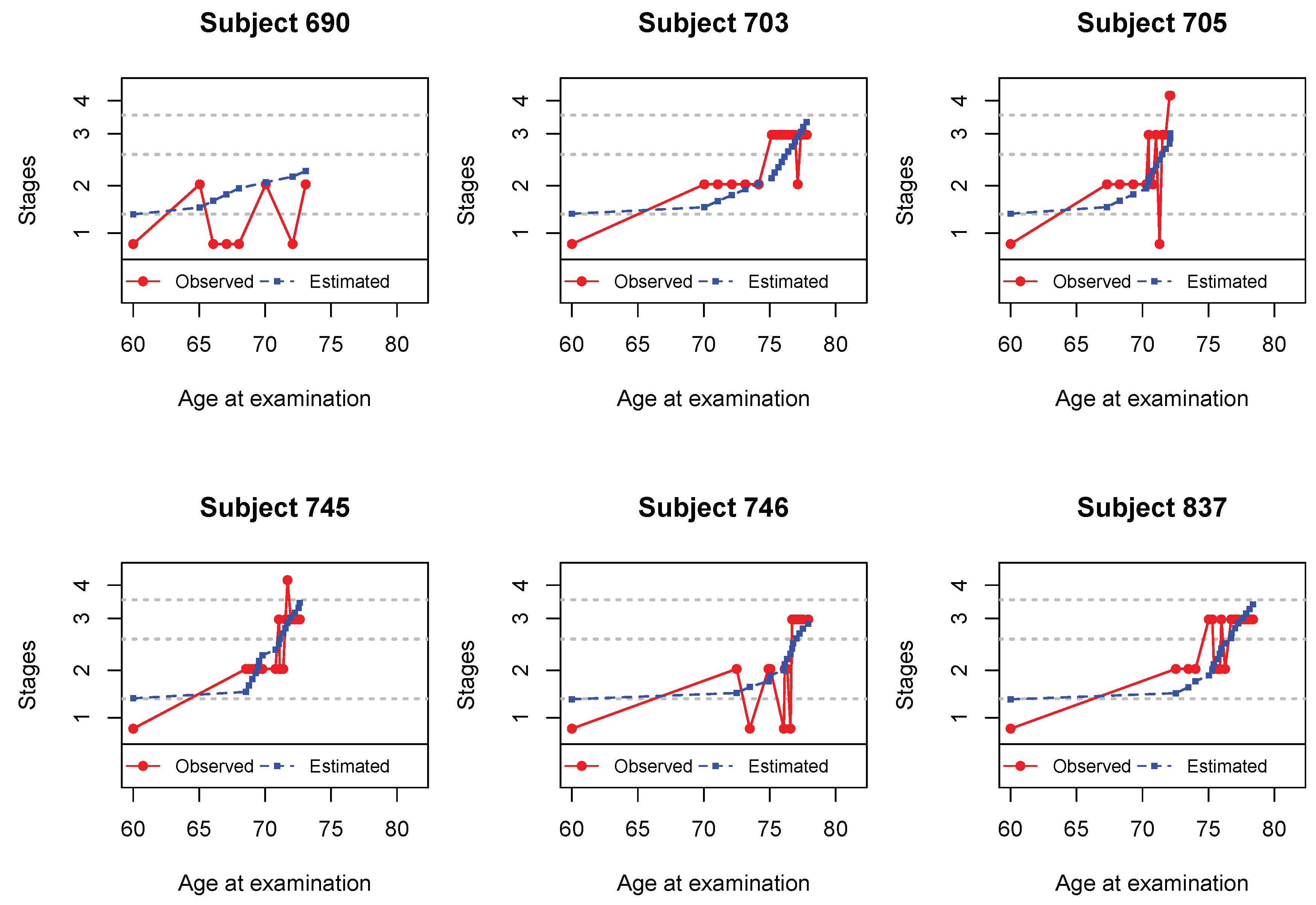
Figure 3 shows the observed and estimated trajectories for six subjects with measurement errors. The estimated dots represent the mean of the estimated true responses with non-decreasing patterns $\widehat{w_{ik}}.$ The corrections performed seem to be in agreement with the dynamic progression of the disease. The observed and estimated stages for these subjects are presented in

Table 7. Aneurysm data: observed and estimated stages for six subjects.

Subject	Age	60.0	65.0	66.1	67.1	68.0	70.1	72.1	73.1
690	Observed	1	2	1	1	1	2	1	2
	Estimated	1	2	2	2	2	2	2	2
Subject	Age	60.0	70.0	71.1	72.1	73.2	74.2	75.2	75.4	75.7	75.9	76.1	76.4	76.7	76.9	77.1	77.4	77.6	77.8
703	Observed	1	2	2	2	2	2	3	3	3	3	3	3	3	3	2	3	3	3
	Estimated	1	2	2	2	2	2	2	2	2	2	2	3	3	3	3	3	3	3
Subject	Age	60.0	67.3	68.3	69.3	70.3	70.5	70.5	70.8	71.0	71.3	71.5	71.8	72.1	72.1	72.1
705	Observed	1	2	2	2	2	3	2	2	3	1	3	3	4	4	4
	Estimated	1	2	2	2	2	2	2	2	2	2	3	3	3	3	3
Subject	Age	60.0	68.6	68.8	69.0	69.3	69.5	69.6	69.8	70.8	71.0	71.1	71.4	71.5	71.7	71.9	72.3	72.5	72.6
745	Observed	1	2	2	2	2	2	2	2	2	3	2	2	3	4	3	3	3	3
	Estimated	1	2	2	2	2	2	2	2	2	2	3	3	3	3	3	3	3	3
Subject	Age	60.0	72.5	73.5	74.9	75.0	76.1	76.1	76.3	76.6	76.7	76.8	77.0	77.3	77.5	77.9
746	Observed	1	2	1	2	2	1	2	2	1	3	3	3	3	3	3
	Estimated	1	2	2	2	2	2	2	2	2	2	2	3	3	3	3
Subject	Age	60.0	72.5	73.5	74.0	75.0	75.3	75.4	75.7	75.9	76.0	76.3	76.7	76.8	77.0	77.3	77.6	77.9	78.1	78.4
837	Observed	1	2	2	2	3	3	2	2	2	3	2	3	3	3	3	3	3	3	3
	Estimated	1	2	2	2	2	2	2	2	2	2	2	3	3	3	3	3	3	3	3

.

A cross-validation scheme was considered to assess the model generalization performance. The 207 subjects were randomly divided into a training set with $75\%$ (155 subjects) and a testing set with $25\%$ (52 subjects). The approach was applied to the training set of subjects, and the model parameters were estimated, then applied to the subjects in the testing set, so that the estimated measurements and stages could be calculated. This was repeated 100 times, and the results were averaged.

Table 8. Aneurysm data: relative frequencies of transitions between stages of aortic diameter with cross-validation.

Relative		Stages at Time ${\mathit{t}}_{\mathit{i},\mathit{k}+1}$
Frequencies		Stage 1	Stage 2	Stage 3	Stage 4
Stages	Stage 1	0.0688	0.0889	0	0
at	Stage 2	0	0.7723	0.0166	0
time	Stage 3	0	0	0.0517	0.0009
$t_{ik}$	Stage 4	0	0	0	0.0008

shows the relative frequencies of transitions under this cross-validation scheme.

This cross-validation allowed predicting the fit of the proposed model to hypothetical test data. These predictions only showed non-decreasing patterns, i.e.: subjects in Stage 1 remained in Stage 1 or went to Stage 2; subjects in Stage 2 remained in Stage 2 or went to Stage 3; subjects in Stage 3 remained in Stage 3 or went to Stage 4; and finally, subjects in Stage 4 remained in Stage 4. It can also be observed that from one time to another, no more than one stage was increased. Both non-decreasing patterns and increasing one stage at a time were compatible with the degenerative nature of this disease.

Using all the subjects as training data may have resulted in model overfitting, which is the effect of overtraining a learning algorithm with certain data. Cross-validation provides a better indication of how well a model will perform on unseen data. In this case, the results with cross-validation presented in Table 8 supported those obtained in Table 6, since the results were close. In order to quantify this closeness, the average of the differences in the absolute value between the elements in both matrices was considered. This average was 0.0139, which in percentage terms represented 1.39%.

6. Conclusions

An inhomogeneous continuous hidden Markov model was defined, developed, and implemented to address measurement errors in ordinal response and monotonic non-decreasing processes. An efficient MCMC algorithm was derived and tested on a simulation-based experiment and applied to aortic aneurysm data. Although the approach was motivated by the aortic aneurysm progression problem, it is applicable to any monotonic non-decreasing process whose ordinal response variable is subject to measurement errors.

The predominant pathologic feature of abdominal aortic aneurysm is elastin destruction, which leads to an abnormal bulge in the aorta walls. Errors are produced when measuring the diameter of the aorta in the affected area. Some of the measurements show decreasing patterns through time, which are not possible since this disease has a degenerative nature. The proposed approach provided information about the progression process through the regression parameters and about the degree of error made through the standard deviation parameters. The corrections performed seemed to be in agreement with the dynamic progression of the disease.

As a future research line, the approach could be modified to consider other experimental designs such as considering that several examiners recorded the responses or using different ways of measuring. This would imply the inclusion of new parameters in the model, which slightly change the implementation. Moreover, different specifications of the regression parameters or the variance parameters could also be considered to build heterogeneity models. In addition, the proposed model could also be modified to handle monotonic non-increasing responses.