Robust Dissipativity Analysis of Hopfield-Type Complex-Valued Neural Networks with Time-Varying Delays and Linear Fractional Uncertainties

Abstract

We study the robust dissipativity issue with respect to the Hopfield-type of complex-valued neural network (HTCVNN) models incorporated with time-varying delays and linear fractional uncertainties. To avoid the computational issues in the complex domain, we divide the original complex-valued system into two real-valued systems. We devise an appropriate Lyapunov-Krasovskii functional (LKF) equipped with general integral terms to facilitate the analysis. By exploiting the multiple integral inequality method, the sufficient conditions for the dissipativity of HTCVNN models are obtained via the linear matrix inequalities (LMIs). The MATLAB software package is used to solve the LMIs effectively. We devise a number of numerical models and their empirical results positively ascertain the obtained results.

1. Introduction

Nowadays, many investigations related to the dynamical properties with respect to a variety of complex-valued neural network (CVNN) models have been published in the literature. In the engineering science domain, the applications of CVNN models have been reported by many researchers, e.g., for sonic wave, electromagnetic wave, light wave, quantum devices, image processing as well as signal processing. In regard to both the mathematical analysis and practical application, CVNN models have been widely studied, and many effective methods on various dynamical analysis of CVNN models are available [1,2,3,4,5,6,7,8,9,10,11,12,13,14,15]. Mainly, the Hopfield-type of neural network (HTNN) models has been considered a key development owing to their adaptive mathematical model capability, along with many powerful methods concerning the stability of HTNN models [1,13,16,17,18].

Time delays naturally occur in almost every dynamical system, which could cause the unstable behaviors of the resulting system [19,20,21,22,23,24,25]. Because of these characteristics, the stability of delayed NN models has been highly focused, resulting in many research studies with comprehensive results [26,27,28,29,30,31,32,33,34,35,36,37,38,39]. On the other hand, it is important to investigate the stability of NN models with the effects of linear fractional uncertainties. Because, when practical systems are modelled, uncertainties of system parameters are often included. From the application point of view, it is important to investigate NN models with linear fractional uncertainties. Several methods for analyzing the dynamical properties of NN models with linear fractional uncertainties have recently been proposed [23,24,39]. By using the Lyapunov function, the robust stability of delayed NN models has been studied with linear fractional uncertainties [23]. In [39], several sufficient conditions have been derived. The study focuses on impulsive NN models, whereby the problem of state feedback synchronization control considering linear fractional uncertainties along with mixed delays has been tackled.

An essential property pertaining to dynamical systems is the dissipativity theory. It provides more knowledge than stability. This is because stability analysis is normally strictly related to the phenomenon of energy dissipation or loss. Besides that, the dissipativity theory offers a critical methodology for designing control systems through an input–output representation using system energy-related contemplations. As a result, many publications on the dissipativity analysis of NN models are available in the literature [26,27,28,29,30,31,32,33,34,35,36,37,40]. As an example, a number of new conditions with respect to the $(\mathbf{Q},\mathbf{S},\mathbf{R})$ dissipativity criteria, global exponential dissipativity, and global dissipativity have been developed for a class of CVNN models in [31,37]. In [32], the use of Dini derivative concepts has resulted in novel sufficient conditions for the dissipativity of complex-valued bi-directional associative memory NN models. The dissipativity of discrete-time systems has been studied in [34]. A new concept of dissipativity has been introduced to describe the changes in subsystems and dissipation of energy of the considered system. Most of the existing studies treat the global dissipativity analysis of CVNN models under the global attractive set. With respect to HTCVNN models, the underlying challenge pertaining to $(\mathbf{Q},\mathbf{S},\mathbf{R})$ dissipativity analysis has yet to be fully considered, which is a key research area.

In this paper, we design novel dissipativity criteria with respect to the HTCVNN models taking into consideration both time-varying delays and linear fractional uncertainties by utilizing the Lyapunov stability theory. To tackle the task, we devise an appropriate delay-dependent Lyapunov-Krasovskii functional (LKF) incorporating general integral terms as well as utilize linear matrix inequality (LMI) and multiple integral inequality to derive the sufficient conditions pertaining to dissipativity of the HTCVNN models. In particular, unlike some traditional dissipativity analysis of CVNN models, we establish new LMI-based dissipativity conditions by forming two equivalent real-valued NN models from a CVNN model. Through several numerical examples, we demonstrate the usefulness of the results.

The remaining paper is arranged as follows. In Section 2, we define the problem statement formally. We express the main results and the numerical examples in Section 3 and Section 4, respectively. The conclusions are presented in Section 5.

Notations: The Euclidean n-space, $n\times n$ real matrices are denoted by ${\mathbb{R}}^n,{\mathbb{R}}^{n\times n}$, while the n dimensional complex vectors, $n\times n$ complex matrices are denoted by ${\mathbb{C}}^n,{\mathbb{C}}^{n\times n}$, respectively. The imaginary unit is denoted by i, where $i=\sqrt{-1}$, and the induced matrix 2-norm is denoted by $\parallel ·\parallel$. The complex conjugate transpose and matrix transposition are donated by the superscripts * and T. Given matrix $\mathcal{P}$, a positive (negative) definite matrix is denoted by $\mathcal{P}>0(\mathcal{P}<0)$. In addition, an identity matrix is denoted by $\mathcal{I}$, while the diagonal of a block diagonal matrix is denoted by $diag\{·\}$. Given a Hermitian matrix, the conjugate transpose of the block is denoted by ★, while $\divideontimes$ denotes the symmetric terms in a matrix.

2. Problem Statement and Fundamentals

Given a CVHNN model with time-varying delays is expressed as

$$\begin{array}{c}\left\{\begin{array}{cc}{\dot{p}}_x\left(t\right)=\hfill & -{\mathbf{d}}_x{p}_x\left(t\right)+{\displaystyle \sum _{y=1}^n}{\mathbf{a}}_{xy}{g}_y\left(p_y(t-r\left(t\right))\right)+u_x\left(t\right),\hfill \\ q_x\left(t\right)=\hfill & g_x\left(p_x\left(t\right)\right),\hfill \\ p_x\left(t\right)=\hfill & {\varphi }_x\left(t\right),t\in [-r,0],x=1,\dots ,n,\hfill \end{array}\right.\hfill \end{array}$$

(1)

or

$$\begin{array}{c}\left\{\begin{array}{cc}\dot{p}\left(t\right)=\hfill & -\mathcal{D}p\left(t\right)+\mathcal{A}g\left(p\right(t-r\left(t\right)\left)\right)+u\left(t\right),\hfill \\ q\left(t\right)=\hfill & g\left(p\right(t\left)\right),\hfill \\ p\left(t\right)=\hfill & \varphi \left(t\right),t\in [-r,0],\hfill \end{array}\right.\hfill \end{array}$$

(2)

under the following assumptions:

$\left({\mathbf{A}}_1\right)$: The state vector is $p\left(t\right)\in {\mathbb{C}}^n$; the disturbance input vector is $u\left(t\right)\in {\mathbb{C}}^n$; the output vector is $q\left(t\right)\in {\mathbb{C}}^n$; the delayed connection weight matrix and the self-feedback connection weight matrix are $\mathcal{A}={\left[{\mathbf{a}}_{xy}\right]}_{n\times n}\in {\mathbb{C}}^{n\times n}$ and $\mathcal{D}=diag\{{\mathbf{d}}_1,\dots ,{\mathbf{d}}_n\}\in {\mathbb{R}}^n$ with ${\mathbf{d}}_x>0$, respectively; while the initial condition is $\varphi \left(t\right)$.

$\left({\mathbf{A}}_2\right)$: The activation function $g_y(·),y=1,\dots ,n$ satisfies the following Lipschitz condition for all $p_1,p_2\in \mathbb{C}$

$$\begin{array}{c}|g_y\left(p_1\right)-g_y\left(p_2\right)|\le l_y|p_1-p_2|,y=1,\dots ,n,\hfill \end{array}$$

(3)

where $l_y$ is a constant.

$\left({\mathbf{A}}_3\right)$: The time-varying delay function is $r\left(t\right)$, which satisfies

$$\begin{array}{c}0\le r\left(t\right)\le r,\dot{r}\left(t\right)\le \mu ,\hfill \end{array}$$

(4)

where $\mu$ and r are known constants.

It should be remembered that the uncertainties associated with the weight coefficients of neurons are unavoidable in network models. Therefore, the parameter uncertainties cannot be overlooked when analyzing the stability of NN models. Therefore, the UHTCVNN model can be described by

$$\begin{array}{c}\left\{\begin{array}{cc}\dot{p}\left(t\right)=\hfill & -(\mathcal{D}+\Delta \mathcal{D}(t\left)\right)p\left(t\right)+(\mathcal{A}+\Delta \mathcal{A}(t\left)\right)g\left(p\right(t-r\left(t\right)\left)\right)+u\left(t\right),\hfill \\ q\left(t\right)=\hfill & g\left(p\right(t\left)\right),\hfill \\ p\left(t\right)=\hfill & \varphi \left(t\right),t\in [-r,0].\hfill \end{array}\right.\hfill \end{array}$$

(5)

Note that $\Delta \mathcal{D}\left(t\right),\Delta \mathcal{A}\left(t\right)=\Delta {\mathcal{A}}^R\left(t\right)+i\Delta {\mathcal{A}}^I\left(t\right)$ in (5) are the parameter uncertainties, and they satisfy:

$$\begin{array}{cc}\left[\Delta \mathcal{D}\left(t\right),\Delta {\mathcal{A}}^R\left(t\right),\Delta {\mathcal{A}}^I\left(t\right)\right]=\hfill & \mathcal{G}\Delta \left(t\right)\left[{\mathcal{H}}_1,{\mathcal{H}}_2,{\mathcal{H}}_3\right],\hfill \end{array}$$

(6)

$$\begin{array}{cc}\Delta \left(t\right)=\hfill & {(\mathcal{I}-\mathcal{J}\mathcal{F}\left(t\right))}^{-1}\mathcal{F}\left(t\right),\hfill \end{array}$$

(7)

$$\begin{array}{cc}\mathcal{I}-{\mathcal{J}}^T\mathcal{J}>\hfill & 0.\hfill \end{array}$$

(8)

where the known constant real matrices are $\mathcal{G},{\mathcal{H}}_1,{\mathcal{H}}_2,{\mathcal{H}}_3$ and $\mathcal{J}$; the time-varying uncertain matrix is $\mathcal{F}\left(t\right)$, which satisfies

$$\begin{array}{c}{\mathcal{F}}^T\left(t\right)\mathcal{F}\left(t\right)\le \mathcal{I}.\hfill \end{array}$$

(9)

Remark 1.

From the inequalities (8) and (9), it is confirmed that $(\mathcal{I}-\mathcal{J}\mathcal{F}(t\left)\right)$ is invertible. Given $\mathcal{J}=0$, the following norm-bounded parametric uncertainty form ${\Delta }^T\left(t\right)\Delta \left(t\right)={\mathcal{F}}^T\left(t\right)\mathcal{F}\left(t\right)\le \mathcal{I}$ can be obtained from the linear fractional uncertainty of the form (6).

For a comprehensive analysis, let $p\left(t\right)=x\left(t\right)+iy\left(t\right),\mathcal{A}={\mathcal{A}}^R+i{\mathcal{A}}^I,g\left(p(t-r\left(t\right))\right)=g^R(x(t-r\left(t\right)),y(t-r\left(t\right)))+i{g}^I(x(t-r\left(t\right)),y(t-r\left(t\right))),u\left(t\right)=u^R\left(t\right)+i{u}^I\left(t\right),q\left(t\right)=q^R\left(t\right)+i{q}^I\left(t\right)$, where the imaginary unit is i.

The real and imaginary parts of the HTCVNN model in (5) are

$$\begin{array}{c}\left\{\begin{array}{cc}\hfill & dx\left(t\right)=[-(\mathcal{D}+\Delta \mathcal{D}\left(t\right))x\left(t\right)+({\mathcal{A}}^R+\Delta {\mathcal{A}}^R\left(t\right))g^R(x(t-r\left(t\right)),\hfill \\ \hfill & y(t-r\left(t\right)))-({\mathcal{A}}^I+\Delta {\mathcal{A}}^I\left(t\right))g^I(x(t-r\left(t\right)),y(t-r\left(t\right)))+u^R\left(t\right)]dt,\hfill \\ \hfill & dy\left(t\right)=[-(\mathcal{D}+\Delta \mathcal{D}\left(t\right))y\left(t\right)+({\mathcal{A}}^I+\Delta {\mathcal{A}}^I\left(t\right))g^R(x(t-r\left(t\right)),y(t-r\left(t\right)))\hfill \\ \hfill & +({\mathcal{A}}^R+\Delta {\mathcal{A}}^R\left(t\right))g^I(x(t-r\left(t\right)),y(t-r\left(t\right)))+u^I\left(t\right)]dt,\hfill \\ \hfill & q^R\left(t\right)=g^R(x\left(t\right),y\left(t\right)),\hfill \\ \hfill & q^I\left(t\right)=g^I(x\left(t\right),y\left(t\right)).\hfill \end{array}\right.\hfill \end{array}$$

(10)

From (10), an equivalent form of the model is

$$\begin{array}{c}\left\{\begin{array}{cc}\left[\begin{array}{c}dx\left(t\right)\\ dy\left(t\right)\end{array}\right]=\hfill & [-\left[\begin{array}{cc}\mathcal{D}+\Delta \mathcal{D}\left(t\right)& 0\\ 0& \mathcal{D}+\Delta \mathcal{D}\left(t\right)\end{array}\right]\left[\begin{array}{c}x\left(t\right)\\ y\left(t\right)\end{array}\right]+\left[\begin{array}{cc}{\mathcal{A}}^R+\Delta {\mathcal{A}}^R\left(t\right)& -{\mathcal{A}}^I-\Delta {\mathcal{A}}^I\left(t\right)\\ {\mathcal{A}}^I+\Delta {\mathcal{A}}^I\left(t\right)& {\mathcal{A}}^R+\Delta {\mathcal{A}}^R\left(t\right)\end{array}\right]\hfill \\ & \times \left[\begin{array}{c}{g}^R(x(t-r\left(t\right)),y(t-r\left(t\right)))\\ g^I(x(t-r\left(t\right)),y(t-r\left(t\right)))\end{array}\right]+\left[\begin{array}{c}{u}^R\left(t\right)\\ u^I\left(t\right)\end{array}\right]]dt,\hfill \\ \left[\begin{array}{c}{q}^R\left(t\right)\\ q^I\left(t\right)\end{array}\right]=\hfill & \left[\begin{array}{c}{g}^R(x\left(t\right),y\left(t\right))\\ g^I(x\left(t\right),y\left(t\right))\end{array}\right],\hfill \end{array}\right.\hfill \end{array}$$

(11)

which is equivalent to

$$\begin{array}{c}\left\{\begin{array}{cc}\left[\begin{array}{c}dx\left(t\right)\\ dy\left(t\right)\end{array}\right]=\hfill & [-\left[\left[\begin{array}{cc}\mathcal{D}& 0\\ 0& \mathcal{D}\end{array}\right]+\left[\begin{array}{cc}\Delta \mathcal{D}\left(t\right)& 0\\ 0& \Delta \mathcal{D}\left(t\right)\end{array}\right]\right]\left[\begin{array}{c}x\left(t\right)\\ y\left(t\right)\end{array}\right]+[\left[\begin{array}{cc}{\mathcal{A}}^R& -{\mathcal{A}}^I\\ {\mathcal{A}}^I& {\mathcal{A}}^R\end{array}\right]\hfill \\ & +\left[\begin{array}{cc}\Delta {\mathcal{A}}^R\left(t\right)& -\Delta {\mathcal{A}}^I\left(t\right)\\ \Delta {\mathcal{A}}^I\left(t\right)& \Delta {\mathcal{A}}^R\left(t\right)\end{array}\right]]\left[\begin{array}{c}{g}^R(x(t-r\left(t\right)),y(t-r\left(t\right)))\\ g^I(x(t-r\left(t\right)),y(t-r\left(t\right)))\end{array}\right]+\left[\begin{array}{c}{u}^R\left(t\right)\\ u^I\left(t\right)\end{array}\right]]dt,\hfill \\ \left[\begin{array}{c}{q}^R\left(t\right)\\ q^I\left(t\right)\end{array}\right]=\hfill & \left[\begin{array}{c}{g}^R(x\left(t\right),y\left(t\right))\\ g^I(x\left(t\right),y\left(t\right))\end{array}\right].\hfill \end{array}\right.\hfill \end{array}$$

(12)

Let

$$\begin{array}{cc}\hfill & \tilde{\mathfrak{e}}\left(t\right)=\left[\begin{array}{c}x\left(t\right)\\ y\left(t\right)\end{array}\right],\tilde{u}\left(t\right)=\left[\begin{array}{c}{u}^R\left(t\right)\\ u^I\left(t\right)\end{array}\right],\hfill \\ \hfill & \tilde{g}\left(\tilde{\mathfrak{e}}(t-r\left(t\right))\right)=\left[\begin{array}{c}{g}^R(x(t-r\left(t\right)),y(t-r\left(t\right)))\\ g^I(x(t-r\left(t\right)),y(t-r\left(t\right)))\end{array}\right],\hfill \\ \hfill & \tilde{g}\left(\tilde{\mathfrak{e}}\left(t\right)\right)=\left[\begin{array}{c}{g}^R(x\left(t\right),y\left(t\right))\\ g^I(x\left(t\right),y\left(t\right))\end{array}\right],\tilde{\mathfrak{z}}\left(t\right)=\left[\begin{array}{c}{q}^R\left(t\right)\\ q^I\left(t\right)\end{array}\right],\hfill \\ \hfill & \tilde{\mathcal{D}}=\left[\begin{array}{cc}\mathcal{D}& 0\\ 0& \mathcal{D}\end{array}\right],\tilde{\mathcal{A}}=\left[\begin{array}{cc}{\mathcal{A}}^R& -{\mathcal{A}}^I\\ {\mathcal{A}}^I& {\mathcal{A}}^R\end{array}\right],\hfill \end{array}$$

$$\begin{array}{cc}\hfill & \Delta \tilde{\mathcal{D}}=\left[\begin{array}{cc}\Delta \mathcal{D}\left(t\right)& 0\\ 0& \Delta \mathcal{D}\left(t\right)\end{array}\right],\hfill \\ \hfill & \Delta \tilde{\mathcal{A}}=\left[\begin{array}{cc}\Delta {\mathcal{A}}^R\left(t\right)& -\Delta {\mathcal{A}}^I\left(t\right)\\ \Delta {\mathcal{A}}^I\left(t\right)& \Delta {\mathcal{A}}^R\left(t\right)\end{array}\right].\hfill \end{array}$$

Then, we can express the model in (12) in an equivalent form of

$$\begin{array}{c}\left\{\begin{array}{cc}d\tilde{\mathfrak{e}}\left(t\right)=\hfill & [-(\tilde{\mathcal{D}}+\Delta \tilde{\mathcal{D}})\tilde{\mathfrak{e}}\left(t\right)+(\tilde{\mathcal{A}}+\Delta \tilde{\mathcal{A}})\tilde{g}\left(\tilde{\mathfrak{e}}(t-r\left(t\right))\right)+\tilde{u}\left(t\right)]dt,\hfill \\ \tilde{\mathfrak{z}}\left(t\right)=\hfill & \tilde{g}\left(\tilde{\mathfrak{e}}\left(t\right)\right).\hfill \end{array}\right.\hfill \end{array}$$

(13)

From (6)–(8), the parameter uncertainties $\Delta \tilde{\mathcal{D}},\Delta \tilde{\mathcal{A}}$ satisfy:

$$\begin{array}{cc}\left[\Delta \tilde{\mathcal{D}},\Delta \tilde{\mathcal{A}}\right]=\hfill & \tilde{\mathcal{G}}\tilde{\Delta }\left(t\right)\left[{\tilde{\mathcal{H}}}_1,{\tilde{\mathcal{H}}}_2\right],\hfill \end{array}$$

(14)

$$\begin{array}{cc}\tilde{\Delta }\left(t\right)=\hfill & {(\tilde{\mathcal{I}}-\tilde{\mathcal{J}}\tilde{\mathcal{F}}\left(t\right))}^{-1}\tilde{\mathcal{F}}\left(t\right),\hfill \end{array}$$

(15)

$$\begin{array}{cc}\tilde{\mathcal{I}}-{\tilde{\mathcal{J}}}^T\tilde{\mathcal{J}}>\hfill & 0.\hfill \end{array}$$

(16)

where

$$\begin{array}{cc}\tilde{\mathcal{G}}=\hfill & \left[\begin{array}{cc}\mathcal{G}& 0\\ 0& \mathcal{G}\end{array}\right],\tilde{\Delta }\left(t\right)=\left[\begin{array}{cc}\Delta \left(t\right)& 0\\ 0& \Delta \left(t\right)\end{array}\right],{\tilde{\mathcal{H}}}_1=\left[\begin{array}{cc}{\mathcal{H}}_1& 0\\ 0& {\mathcal{H}}_1\end{array}\right].{\tilde{\mathcal{H}}}_2=\left[\begin{array}{cc}{\mathcal{H}}_2& -{\mathcal{H}}_3\\ {\mathcal{H}}_3& {\mathcal{H}}_2\end{array}\right],\hfill \\ \tilde{\mathcal{F}}\left(t\right)=\hfill & \left[\begin{array}{cc}\mathcal{F}\left(t\right)& 0\\ 0& \mathcal{F}\left(t\right)\end{array}\right],\tilde{\mathcal{I}}=\left[\begin{array}{cc}\mathcal{I}& 0\\ 0& \mathcal{I}\end{array}\right],\tilde{\mathcal{J}}=\left[\begin{array}{cc}\mathcal{J}& 0\\ 0& \mathcal{J}\end{array}\right].\hfill \end{array}$$

According to $\left({\mathbf{A}}_2\right)$, it is straightforward to obtain

$$\begin{array}{cc}{(g\left(z_1\right)-g\left(z_2\right))}^{\ast }\hfill & (g\left(z_1\right)-g\left(z_2\right))\le {(z_1-z_2)}^{\ast }{\mathcal{L}}^T\mathcal{L}(z_1-z_2),\hfill \end{array}$$

(17)

where $\mathcal{L}=diag\{l_1,\dots ,l_n\}$.

The real and imaginary parts of Equation (17) are

$$\begin{array}{cc}{(\tilde{g}\left({\tilde{\mathfrak{e}}}_1\right)-\tilde{g}\left({\tilde{\mathfrak{e}}}_2\right))}^T\hfill & (\tilde{g}\left({\tilde{\mathfrak{e}}}_1\right)-\tilde{g}\left({\tilde{\mathfrak{e}}}_2\right))\le {({\tilde{\mathfrak{e}}}_1-{\tilde{\mathfrak{e}}}_2)}^T\tilde{\mathcal{L}}({\tilde{\mathfrak{e}}}_1-{\tilde{\mathfrak{e}}}_2),\hfill \end{array}$$

(18)

where $\tilde{\mathcal{L}}=\left[\begin{array}{cc}{\mathcal{L}}^T\mathcal{L}& 0\\ 0& {\mathcal{L}}^T\mathcal{L}\end{array}\right]$.

Given the model in (13), the initial condition is

$$\begin{array}{c}\tilde{\mathfrak{e}}\left(t\right)=\tilde{\varphi }\left(t\right),t\in [-r,0],\hfill \end{array}$$

(19)

where $\tilde{\varphi }\left(t\right)={[{\varphi }^R\left(t\right),{\varphi }^I\left(t\right)]}^T$.

Remark 2.

It should be noted that, if we let $\Delta \tilde{\mathcal{D}}=\Delta \tilde{\mathcal{A}}=0$, the NN model in (13) becomes

$$\begin{array}{c}\left\{\begin{array}{cc}d\tilde{\mathfrak{e}}\left(t\right)=\hfill & [-\tilde{\mathcal{D}}\tilde{\mathfrak{e}}\left(t\right)+\tilde{\mathcal{A}}\tilde{g}\left(\tilde{\mathfrak{e}}(t-r\left(t\right))\right)+\tilde{u}\left(t\right)]dt,\hfill \\ \tilde{\mathfrak{z}}\left(t\right)=\hfill & \tilde{g}\left(\tilde{\mathfrak{e}}\left(t\right)\right)\hfill \end{array}\right.\hfill \end{array}$$

(20)

The real-valued NN model in (20) is an equivalent form of the original model in (2). In addition, the model in (5) is an equivalent form of the real-valued NN model in (13).

A number of key lemmas and definitions used to derive the main results are explained.

Definition 1

([31]). Given the existence of a compact set $\mathbb{S}\subseteq {\mathbb{C}}^n$, whereby $\forall p_0\in {\mathbb{C}}^n,\exists T>0$, when $t\ge t_0+T,p(t,t_0,p_0)\subseteq \mathbb{S}$ in which the solution of (5) from the initial state and time of $p_0$ is denoted by $p(t,t_0,p_0)$, the CVNN model in (5) is said to be globally dissipative. In this case, $\mathbb{S}$ is called a globally attractive set. A set $\mathbb{S}$ is called positive invariant if $\forall p_0\in \mathbb{S}$ implies $p(t,t_0,p_0)\subseteq \mathbb{S}$ for $t\ge t_0$.

Similar to the publications in [31,34,35,37], the energy supply function for the NN model in (5) is defined as

$$\begin{array}{c}\mathbf{G}(u,q,\mathcal{T})={⟨q,\mathbf{Q}q⟩}_{\mathcal{T}}+2{⟨q,\mathbf{S}u⟩}_{\mathcal{T}}+{⟨u,\mathbf{R}u⟩}_{\mathcal{T}},\hfill \end{array}$$

(21)

where $\mathbf{Q}\le 0$, and $\mathbf{Q},\mathbf{S},\mathbf{R}\in {\mathbb{C}}^{n\times n}$. In addition,

$$\begin{array}{c}{⟨a,b⟩}_{\mathcal{T}}={\int }_0^{\mathcal{T}}{a}^{T}bdt,\mathcal{T}\ge 0.\hfill \end{array}$$

Definition 2

([31,37]). Subject to zero initial state, and given any $\mathcal{T}\ge 0$ and scalar $\alpha >0$, under zero initial state, the CVNN model in (5) is said to be strictly $(\mathbf{Q},\mathbf{S},\mathbf{R})$-dissipative. The following inequality

$$\begin{array}{c}\mathbf{G}(u,q,\mathcal{T})\ge \alpha {⟨u,u⟩}_{\mathcal{T}},\hfill \end{array}$$

(22)

holds with respect to any non-zero input $u\in {\mathbf{L}}_2[0,\infty )$.

For the model in (5), we can express the relation (22) in an equivalent dissipativity performance index, as follows:

$$\begin{array}{cc}{\mathbf{J}}_{\alpha ,\mathcal{T}}=\hfill & {\int }_0^{\mathcal{T}}\left[{\left[\begin{array}{c}q\left(t\right)\\ u\left(t\right)\end{array}\right]}^{\ast }\left[\begin{array}{cc}\mathbf{Q}& \mathbf{S}\\ ★& \mathbf{R}\end{array}\right]\left[\begin{array}{c}q\left(t\right)\\ u\left(t\right)\end{array}\right]-\alpha u{\left(t\right)}^{\ast }u\left(t\right)\right]dt.\hfill \end{array}$$

(23)

Remark 3.

We notice from the available publications that a number of definitions for strictly $(\mathbf{Q},\mathbf{S},\mathbf{R})$-dissipativity [27,30], global exponential disspativity and global dissipativity [31,33] are provided in the Euclidean space ${\mathbb{R}}^n$. These definitions have been extended in recent publication [31,34,35,36,37] to the complex plane ${\mathbb{C}}^n$.

At the same time, the energy supply function for the NN model in (13) can be defined as follows:

$$\begin{array}{c}\mathbf{G}(\tilde{u},\tilde{\mathfrak{z}},\mathcal{T})={⟨\tilde{\mathfrak{z}},\tilde{\mathbf{Q}}\tilde{\mathfrak{z}}⟩}_{\mathcal{T}}+2{⟨\tilde{\mathfrak{z}},\tilde{\mathbf{S}}\tilde{u}⟩}_{\mathcal{T}}+{⟨\tilde{u},\tilde{\mathbf{R}}\tilde{u}⟩}_{\mathcal{T}},\hfill \end{array}$$

(24)

where $\tilde{\mathbf{Q}},\tilde{\mathbf{S}},\tilde{\mathbf{R}}\in {\mathbb{R}}^{n\times n}$, and

$$\begin{array}{c}{⟨a,b⟩}_{\mathcal{T}}={\int }_0^{\mathcal{T}}{a}^{T}bdt,\mathcal{T}\ge 0.\hfill \end{array}$$

Definition 3.

Given scalar $\alpha >0$ and $\mathcal{T}\ge 0$, and subject to zero initial condition, the NN model in (13) is said to be strictly $(\tilde{\mathbf{Q}},\tilde{\mathbf{S}},\tilde{\mathbf{R}})$-dissipative. The following inequality

$$\begin{array}{c}\mathbf{G}(\tilde{u},\tilde{q},\mathcal{T})\ge \alpha {⟨\tilde{u},\tilde{u}⟩}_{\mathcal{T}},\hfill \end{array}$$

(25)

holds for any nonzero input $\tilde{u}\in {\mathbf{L}}_2[0,\infty )$.

Consider the NN model in (13), by dividing into the real and imaginary parts, we can write the Inequality (25)

$$\begin{array}{cc}{\mathbf{J}}_{\alpha ,\mathcal{T}}=\hfill & {\int }_0^{\mathcal{T}}\left[{\left[\begin{array}{c}\left[\begin{array}{c}{q}^R\left(t\right)\\ q^I\left(t\right)\end{array}\right]\\ \left[\begin{array}{c}{u}^R\left(t\right)\\ u^I\left(t\right)\end{array}\right]\end{array}\right]}^T\left[\begin{array}{cc}\left[\begin{array}{cc}{\mathbf{Q}}^R& -{\mathbf{Q}}^I\\ {\mathbf{Q}}^I& {\mathbf{Q}}^R\end{array}\right]& \left[\begin{array}{cc}{\mathbf{S}}^R& -{\mathbf{S}}^I\\ {\mathbf{S}}^I& {\mathbf{S}}^R\end{array}\right]\\ \divideontimes & \left[\begin{array}{cc}{\mathbf{R}}^R& -{\mathbf{R}}^I\\ {\mathbf{R}}^I& {\mathbf{R}}^R\end{array}\right]\end{array}\right]\left[\begin{array}{c}\left[\begin{array}{c}{q}^R\left(t\right)\\ q^I\left(t\right)\end{array}\right]\\ \left[\begin{array}{c}{u}^R\left(t\right)\\ u^I\left(t\right)\end{array}\right]\end{array}\right]-\alpha {\left[\begin{array}{c}{u}^R\left(t\right)\\ u^I\left(t\right)\end{array}\right]}^T\left[\begin{array}{c}{u}^R\left(t\right)\\ u^I\left(t\right)\end{array}\right]\right]dt.\hfill \end{array}$$

equivalently

$$\begin{array}{cc}{\mathbf{J}}_{\alpha ,\mathcal{T}}=\hfill & {\int }_0^{\mathcal{T}}\left[{\left[\begin{array}{c}\tilde{\mathfrak{z}}\left(t\right)\\ \tilde{u}\left(t\right)\end{array}\right]}^T\left[\begin{array}{cc}\tilde{\mathbf{Q}}& \tilde{\mathbf{S}}\\ \divideontimes & \tilde{\mathbf{R}}\end{array}\right]\left[\begin{array}{c}\tilde{\mathfrak{z}}\left(t\right)\\ \tilde{u}\left(t\right)\end{array}\right]-\alpha \tilde{u}{\left(t\right)}^T\tilde{u}\left(t\right)\right]dt.\hfill \end{array}$$

(26)

where

$$\begin{array}{c}\tilde{\mathbf{Q}}=\left[\begin{array}{cc}{\mathbf{Q}}^R& -{\mathbf{Q}}^I\\ {\mathbf{Q}}^I& {\mathbf{Q}}^R\end{array}\right],\tilde{\mathbf{S}}=\left[\begin{array}{cc}{\mathbf{S}}^R& -{\mathbf{S}}^I\\ {\mathbf{S}}^I& {\mathbf{S}}^R\end{array}\right],\tilde{\mathbf{R}}=\left[\begin{array}{cc}{\mathbf{R}}^R& -{\mathbf{R}}^I\\ {\mathbf{R}}^I& {\mathbf{R}}^R\end{array}\right].\hfill \end{array}$$

Lemma 1

([38]). Consider scalars ${\mathfrak{s}}_1$ and ${\mathfrak{s}}_2$ satisfying ${\mathfrak{s}}_2-{\mathfrak{s}}_1>0$ and $0\le \mathfrak{n}\in \mathbb{Z}$ and a positive-definite matrix $\mathcal{O}\in {\mathbb{R}}^{n\times n}$. Subject to a continuously differentiable function $\tilde{\mathfrak{e}}:[{\mathfrak{s}}_1,{\mathfrak{s}}_2]\to {\mathbb{R}}^n$, the following inequality holds:

$$\begin{array}{cc}-\frac{{({\mathfrak{s}}_2-{\mathfrak{s}}_1)}^{\mathfrak{n}}}{\mathfrak{n}!}{\int }_{{\mathfrak{s}}_1}^{{\mathfrak{s}}_2}{\int }_{{\mathfrak{z}}_1}^{{\mathfrak{s}}_2}\dots {\int }_{{\mathfrak{z}}_{\mathfrak{n}}}^{{\mathfrak{s}}_2}{\tilde{\mathfrak{e}}}^T\left(\mathfrak{u}\right){\mathcal{O}}_{\mathfrak{n}}\tilde{\mathfrak{e}}\left(\mathfrak{u}\right)d\mathfrak{u}d{\mathfrak{z}}_{\mathfrak{n}}\dots d{\mathfrak{z}}_1\le \hfill & -{\left[{\int }_{{\mathfrak{s}}_1}^{{\mathfrak{s}}_2}{\int }_{{\mathfrak{z}}_1}^{{\mathfrak{s}}_2}\dots {\int }_{{\mathfrak{z}}_{\mathfrak{n}}}^{{\mathfrak{s}}_2}\tilde{\mathfrak{e}}\left(\mathfrak{u}\right)d\mathfrak{u}d{\mathfrak{z}}_{\mathfrak{n}}\dots d{\mathfrak{z}}_1\right]}^T\hfill \\ & \times {\mathcal{O}}_{\mathfrak{n}}\left[{\int }_{{\mathfrak{s}}_1}^{{\mathfrak{s}}_2}{\int }_{{\mathfrak{z}}_1}^{{\mathfrak{s}}_2}\dots {\int }_{{\mathfrak{z}}_{\mathfrak{n}}}^{{\mathfrak{s}}_2}\tilde{\mathfrak{e}}\left(\mathfrak{u}\right)d\mathfrak{u}d{\mathfrak{z}}_{\mathfrak{n}}\dots d{\mathfrak{z}}_1\right].\hfill \end{array}$$

Lemma 2

([39]). Suppose $\Delta \left(t\right)$ is given by (6)–(8). Given $\mathcal{M}$ and $\mathcal{N}$ are of appropriate dimensions and matrix $\mathsf{\Xi }={\mathsf{\Xi }}^T$ the inequality

$$\begin{array}{c}\mathsf{\Xi }+\mathcal{M}\Delta \left(t\right)\mathcal{N}+{(\mathcal{M}\Delta \left(t\right)\mathcal{N})}^T<0,\hfill \end{array}$$

holds for $\mathcal{F}\left(t\right)$ in such a way that ${\mathcal{F}}^T\left(t\right)\mathcal{F}\left(t\right)\le I$ subject to some ϵ, if and only if

$$\begin{array}{c}\left[\begin{array}{ccc}\mathsf{\Xi }& \mathcal{M}& ϵ{\mathcal{N}}^T\\ {\mathcal{M}}^T& -ϵ\mathcal{I}& ϵ{\mathcal{J}}^T\\ ϵ\mathcal{N}& ϵ\mathcal{J}& -ϵ\mathcal{I}\end{array}\right]<0.\hfill \end{array}$$

3. Main Results

The dissipativity analysis of the HTCVNN model in (13) is yet to be fully studied in this literature. To overcome this issue, we derive some sufficient conditions with respect to dissiaptivity pertaining to the NN model in (13). For clarity, we use the following notations:

$$\begin{array}{cc}{\tilde{\mathfrak{e}}}_t:=\hfill & \tilde{\mathfrak{e}}\left(t\right),\hfill \\ {\tilde{\mathfrak{e}}}_{r\left(t\right)}:=\hfill & \tilde{\mathfrak{e}}(t-\mathfrak{r}\left(t\right)),\hfill \\ {\tilde{g}}_t:=\hfill & \tilde{g}\left(\mathfrak{e}\left(t\right)\right),\hfill \\ {\tilde{g}}_{r\left(t\right)}:=\hfill & \tilde{g}\left(\tilde{\mathfrak{e}}(t-\mathfrak{r}\left(t\right))\right),\hfill \end{array}$$

$$\begin{array}{cc}{\tilde{u}}_t:=\hfill & \tilde{u}\left(t\right),\hfill \\ {\tilde{q}}_t:=\hfill & \tilde{q}\left(t\right),\hfill \\ {\tilde{\mathfrak{z}}}_t:=\hfill & \tilde{\mathfrak{z}}\left(t\right),\hfill \\ {\tilde{y}}_t^{\mathfrak{n}}:=\hfill & \sum _{\mathfrak{n}=1}^{\mathfrak{m}}\left[{\int }_{t-r}^t{\int }_{{\mathfrak{z}}_1}^t\dots {\int }_{{\mathfrak{z}}_{\mathfrak{n}-1}}^t\tilde{\mathfrak{e}}\left(\mathfrak{s}\right)d\mathfrak{s}d{\mathfrak{z}}_{\mathfrak{n}-1}\dots d{\mathfrak{z}}_1\right],\hfill \\ {\xi }_t=\hfill & col\left[{\tilde{\mathfrak{e}}}_t{\tilde{\mathfrak{e}}}_{r\left(t\right)}{\tilde{g}}_t{\tilde{g}}_{r\left(t\right)}{\tilde{y}}_t^{\mathfrak{n}}{\tilde{u}}_t\right].\hfill \end{array}$$

Dissipativity Analysis

By employing the Lyapunov stability theory and integral inequality approach, some sufficient conditions are derived. The aim is to make sure the $(\tilde{\mathbf{Q}},\tilde{\mathbf{S}},\tilde{\mathbf{R}})$-$\alpha$ dissipativity of the CVHNN model in (20) in terms of LMIs, as in Theorem 1.

Theorem 1.

Based on Assumption $\left({\mathbf{A}}_2\right)$, we can divide the activation function into both the real and imaginary parts. The NN model in (20) is strictly $(\tilde{\mathbf{Q}},\tilde{\mathbf{S}},\tilde{\mathbf{R}})$-α dissipative subject to scalars $\mu >0$ and $r>0$, and with the existence of scalars $0<{ϵ}_1,0<{ϵ}_2,0<\alpha$ and matrices $0<\mathcal{P},0<\mathcal{Q},0<{\mathcal{R}}_{\mathfrak{n}}(\mathfrak{n}=1,2,\dots \mathfrak{m})$ whereby the following LMI holds:

$$\begin{array}{cc}\tilde{\mho }=\left[\begin{array}{cccccc}{\tilde{\mho }}_1& 0& 0& \mathcal{P}\tilde{\mathcal{A}}& 0& \mathcal{P}\\ \divideontimes & {\tilde{\mho }}_2& 0& 0& 0& 0\\ \divideontimes & \divideontimes & {\tilde{\mho }}_3& 0& 0& -\tilde{\mathbf{S}}\\ \divideontimes & \divideontimes & \divideontimes & -{ϵ}_2\mathcal{I}& 0& 0\\ \divideontimes & \divideontimes & \divideontimes & \divideontimes & -{\mathcal{R}}_{\mathfrak{n}}& 0\\ \divideontimes & \divideontimes & \divideontimes & \divideontimes & \divideontimes & {\tilde{\mho }}_4\end{array}\right]<\hfill & 0,\hfill \end{array}$$

(27)

where ${\tilde{\mho }}_1:=-\mathcal{P}\tilde{\mathcal{D}}-{\tilde{\mathcal{D}}}^T\mathcal{P}+\mathcal{Q}+\sum _{\mathfrak{n}=1}^{\mathfrak{m}}{\left(\frac{r^{\mathfrak{n}}}{\mathfrak{n}!}\right)}^2{\mathcal{R}}_{\mathfrak{n}}+{ϵ}_1\tilde{\mathcal{L}},$ ${\tilde{\mho }}_2:=-(1-\mu )\mathcal{Q}+{ϵ}_2\tilde{\mathcal{L}}$, ${\tilde{\mho }}_3:=-{ϵ}_1\mathcal{I}-\tilde{\mathbf{Q}}$, ${\tilde{\mho }}_4:=-\tilde{\mathbf{R}}+\alpha \mathcal{I}$.

Proof. 

Given the NN model in (20), the following Lyapunov function candidate is considered

$$\begin{array}{cc}\hfill & \mathcal{V}\left(t\right)={\tilde{\mathfrak{e}}}_t^T\mathcal{P}{\tilde{\mathfrak{e}}}_t+{\int }_{t-r\left(t\right)}^t{\tilde{\mathfrak{e}}}^T\left(\mathfrak{s}\right)\mathcal{Q}\tilde{\mathfrak{e}}\left(\mathfrak{s}\right)d\mathfrak{s}+\sum _{\mathfrak{n}=1}^{\mathfrak{m}}\frac{r^{\mathfrak{n}}}{\mathfrak{n}!}{\int }_{t-r}^t{\int }_{{\mathfrak{z}}_1}^t\dots {\int }_{{\mathfrak{z}}_{\mathfrak{n}}}^t{\tilde{\mathfrak{e}}}^T\left(\mathfrak{s}\right){\mathcal{R}}_{\mathfrak{n}}\tilde{\mathfrak{e}}\left(\mathfrak{s}\right)d\mathfrak{s}d{\mathfrak{z}}_{\mathfrak{n}}\dots d{\mathfrak{z}}_1.\hfill \end{array}$$

(28)

We can obtain the time-derivative of $\mathcal{V}\left(t\right)$, i.e.

$$\begin{array}{cc}\dot{\mathcal{V}}\left(t\right)\le \hfill & 2{\tilde{\mathfrak{e}}}_t^T\mathcal{P}[-\tilde{\mathcal{D}}{\tilde{\mathfrak{e}}}_t+\tilde{\mathcal{A}}{\tilde{g}}_{r\left(t\right)}+{\tilde{u}}_t]+{\tilde{\mathfrak{e}}}_t^T\mathcal{Q}{\tilde{\mathfrak{e}}}_t-(1-\mu ){\tilde{\mathfrak{e}}}_{r\left(t\right)}^T\mathcal{Q}{\tilde{\mathfrak{e}}}_{r\left(t\right)}\hfill \\ & +\sum _{\mathfrak{n}=1}^{\mathfrak{m}}\left[{\left(\frac{r^{\mathfrak{n}}}{\mathfrak{n}!}\right)}^2{\tilde{\mathfrak{e}}}_t^T{\mathcal{R}}_{\mathfrak{n}}{\tilde{\mathfrak{e}}}_t-\frac{r^{\mathfrak{n}}}{\mathfrak{n}!}{\int }_{t-r}^t{\int }_{{\mathfrak{z}}_1}^t\dots {\int }_{{\mathfrak{z}}_{\mathfrak{n}-1}}^t{\tilde{\mathfrak{e}}}^T\left(\mathfrak{s}\right){\mathcal{R}}_{\mathfrak{n}}\tilde{\mathfrak{e}}\left(\mathfrak{s}\right)d\mathfrak{s}d{\mathfrak{z}}_{\mathfrak{n}-1}\dots d{\mathfrak{z}}_1\right],\hfill \end{array}$$

(29)

$$\begin{array}{cc}\dot{\mathcal{V}}\left(t\right)\le \hfill & {\tilde{\mathfrak{e}}}_t^T(-\mathcal{P}\tilde{\mathcal{D}}-{\tilde{\mathcal{D}}}^T\mathcal{P}){\tilde{\mathfrak{e}}}_t+{\tilde{\mathfrak{e}}}_t^T\left(\mathcal{P}\tilde{\mathcal{A}}\right){\tilde{g}}_{r\left(t\right)}+{\tilde{\mathfrak{e}}}_t^T\mathcal{P}{\tilde{u}}_t+{\tilde{\mathfrak{e}}}_t^T\mathcal{Q}{\tilde{\mathfrak{e}}}_t-(1-\mu ){\tilde{\mathfrak{e}}}_{r\left(t\right)}^T\mathcal{Q}{\tilde{\mathfrak{e}}}_{r\left(t\right)}\hfill \\ & +\sum _{\mathfrak{n}=1}^{\mathfrak{m}}\left[{\left(\frac{r^{\mathfrak{n}}}{\mathfrak{n}!}\right)}^2{\tilde{\mathfrak{e}}}_t^T{\mathcal{R}}_{\mathfrak{n}}{\tilde{\mathfrak{e}}}_t-\frac{r^{\mathfrak{n}}}{\mathfrak{n}!}{\int }_{t-r}^t{\int }_{{\mathfrak{z}}_1}^t\dots {\int }_{{\mathfrak{z}}_{\mathfrak{n}-1}}^t{\tilde{\mathfrak{e}}}^T\left(\mathfrak{s}\right){\mathcal{R}}_{\mathfrak{n}}\tilde{\mathfrak{e}}\left(\mathfrak{s}\right)d\mathfrak{s}d{\mathfrak{z}}_{\mathfrak{n}-1}\dots d{\mathfrak{z}}_1\right].\hfill \end{array}$$

(30)

We can estimate the terms in (30) through Lemma 1, i.e.,

$$\begin{array}{cc}-\sum _{\mathfrak{n}=1}^{\mathfrak{m}}\frac{r^{\mathfrak{n}}}{\mathfrak{n}!}\left[{\int }_{t-r}^t{\int }_{{\mathfrak{z}}_1}^t\dots {\int }_{{\mathfrak{z}}_{\mathfrak{n}-1}}^t{\tilde{\mathfrak{e}}}^T\left(\mathfrak{s}\right){\mathcal{R}}_{\mathfrak{n}}\tilde{\mathfrak{e}}\left(\mathfrak{s}\right)d\mathfrak{s}d{\mathfrak{z}}_{\mathfrak{n}-1}\dots d{\mathfrak{z}}_1\right]\le \hfill & -\sum _{\mathfrak{n}=1}^{\mathfrak{m}}{\left[{\int }_{t-r}^t{\int }_{{\mathfrak{z}}_1}^t\dots {\int }_{{\mathfrak{z}}_{\mathfrak{n}-1}}^t\tilde{\mathfrak{e}}\left(\mathfrak{s}\right)d\mathfrak{s}d{\mathfrak{z}}_{\mathfrak{n}-1}\dots d{\mathfrak{z}}_1\right]}^T{\mathcal{R}}_{\mathfrak{n}}\hfill \\ & \times \sum _{\mathfrak{n}=1}^{\mathfrak{m}}\left[{\int }_{t-r}^t{\int }_{{\mathfrak{z}}_1}^t\dots {\int }_{{\mathfrak{z}}_{\mathfrak{n}-1}}^t\tilde{\mathfrak{e}}\left(\mathfrak{s}\right)d\mathfrak{s}d{\mathfrak{z}}_{\mathfrak{n}-1}\dots d{\mathfrak{z}}_1\right].\hfill \end{array}$$

(31)

Moreover, from (18), it follows that

$$\begin{array}{cc}0\le \hfill & {ϵ}_1[{\tilde{\mathfrak{e}}}_t^T\tilde{\mathcal{L}}{\tilde{\mathfrak{e}}}_t-{\tilde{g}}_t^T{\tilde{g}}_t],\hfill \end{array}$$

(32)

$$\begin{array}{cc}0\le \hfill & {ϵ}_2[{\tilde{\mathfrak{e}}}_{r\left(t\right)}^T\tilde{\mathcal{L}}{\tilde{\mathfrak{e}}}_{r\left(t\right)}-{\tilde{g}}_{r\left(t\right)}^T{\tilde{g}}_{r\left(t\right)}],\hfill \end{array}$$

(33)

for ${ϵ}_1,{ϵ}_2>0.$

Combining (30)–(33), we have

$$\begin{array}{cc}\dot{\mathcal{V}}\left(t\right)-{\tilde{\mathfrak{z}}}_t^T\tilde{\mathbf{Q}}{\tilde{\mathfrak{z}}}_t-{\tilde{\mathfrak{z}}}_t^T\tilde{\mathbf{S}}{\tilde{u}}_t-{\tilde{u}}_t^T(\tilde{\mathbf{R}}-\alpha \mathcal{I}){\tilde{u}}_t\le \hfill & {\tilde{\mathfrak{e}}}_t^T(-\mathcal{P}\tilde{\mathcal{D}}-{\tilde{\mathcal{D}}}^T\mathcal{P}){\tilde{\mathfrak{e}}}_t+{\tilde{\mathfrak{e}}}_t^T\left(\mathcal{P}\tilde{\mathcal{A}}\right){\tilde{g}}_{r\left(t\right)}+{\tilde{\mathfrak{e}}}_t^T\mathcal{P}{\tilde{u}}_t\hfill \\ & +{\tilde{\mathfrak{e}}}_t^T\mathcal{Q}{\tilde{\mathfrak{e}}}_t-(1-\mu ){\tilde{\mathfrak{e}}}_{r\left(t\right)}^T\mathcal{Q}{\tilde{\mathfrak{e}}}_{r\left(t\right)}+\sum _{\mathfrak{n}=1}^{\mathfrak{m}}[{\left(\frac{r^{\mathfrak{n}}}{\mathfrak{n}!}\right)}^2{\tilde{\mathfrak{e}}}_t^T{\mathcal{R}}_{\mathfrak{n}}{\tilde{\mathfrak{e}}}_t\hfill \\ & -\sum _{\mathfrak{n}=1}^{\mathfrak{m}}{\left[{\int }_{t-r}^t{\int }_{{\mathfrak{z}}_1}^t\dots {\int }_{{\mathfrak{z}}_{\mathfrak{n}-1}}^t\tilde{\mathfrak{e}}\left(\mathfrak{s}\right)d\mathfrak{s}d{\mathfrak{z}}_{\mathfrak{n}-1}\dots d{\mathfrak{z}}_1\right]}^T{\mathcal{R}}_{\mathfrak{n}}\hfill \\ & \times \sum _{\mathfrak{n}=1}^{\mathfrak{m}}\left[{\int }_{t-r}^t{\int }_{{\mathfrak{z}}_1}^t\dots {\int }_{{\mathfrak{z}}_{\mathfrak{n}-1}}^t\tilde{\mathfrak{e}}\left(\mathfrak{s}\right)d\mathfrak{s}d{\mathfrak{z}}_{\mathfrak{n}-1}\dots d{\mathfrak{z}}_1\right]\hfill \\ & +{ϵ}_1{\tilde{\mathfrak{e}}}_t^T\tilde{\mathcal{L}}{\tilde{\mathfrak{e}}}_t-{ϵ}_1{\tilde{g}}_t^T{\tilde{g}}_t+{ϵ}_2{\tilde{\mathfrak{e}}}_{r\left(t\right)}^T\tilde{\mathcal{L}}{\tilde{\mathfrak{e}}}_{r\left(t\right)}-{ϵ}_2{\tilde{g}}_{r\left(t\right)}^T{\tilde{g}}_{r\left(t\right)}\hfill \\ \hfill & \dot{\mathcal{V}}\left(t\right)-{\tilde{\mathfrak{z}}}_t^T\tilde{\mathbf{Q}}{\tilde{\mathfrak{z}}}_t-{\tilde{\mathfrak{z}}}_t^T\tilde{\mathbf{S}}{\tilde{u}}_t-{\tilde{u}}_t^T(\tilde{\mathbf{R}}-\alpha \mathcal{I}){\tilde{u}}_t\le {\tilde{\xi }}_t^T\tilde{\mho }{\tilde{\xi }}_t,\hfill \end{array}$$

(34)

which is equivalent to

$$\dot{\mathcal{V}}\left(t\right)-{\tilde{\mathfrak{z}}}_t^T\tilde{\mathbf{Q}}{\tilde{\mathfrak{z}}}_t-{\tilde{\mathfrak{z}}}_t^T\tilde{\mathbf{S}}{\tilde{u}}_t-{\tilde{u}}_t^T(\tilde{\mathbf{R}}-\alpha \mathcal{I}){\tilde{u}}_t\le {\tilde{\xi }}_t^T\tilde{\mho }{\tilde{\xi }}_t$$

(35)

where $\tilde{\mho }$ is defined in (27), while ${\tilde{\xi }}_t$ is defined in the main results.

From (26), we can obtain

$$\begin{array}{cc}{\mathbf{J}}_{\alpha ,\mathcal{T}}=\hfill & {\int }_0^{\mathcal{T}}\left[{\left[\begin{array}{c}{\tilde{\mathfrak{z}}}_t\\ {\tilde{u}}_t\end{array}\right]}^T\left[\begin{array}{cc}\tilde{\mathbf{Q}}& \tilde{\mathbf{S}}\\ \divideontimes & \tilde{\mathbf{R}}\end{array}\right]\left[\begin{array}{c}{\tilde{\mathfrak{z}}}_t\\ {\tilde{u}}_t\end{array}\right]-\alpha {\tilde{u}}_t^T{\tilde{u}}_t\right]dt.\hfill \end{array}$$

(36)

Suppose $\tilde{\mho }<0$, we have

$$\begin{array}{cc}{\int }_0^{\mathcal{T}}\dot{\mathcal{V}}\left(t\right)dt-{\mathbf{J}}_{\alpha ,\mathcal{T}}\le \hfill & {\int }_0^{\mathcal{T}}{\tilde{\xi }}_t^T\tilde{\mho }{\tilde{\xi }}_{t}dt.\hfill \end{array}$$

(37)

It can be deducted from (27) that

$$\begin{array}{c}{\int }_0^{\mathcal{T}}\dot{\mathcal{V}}\left(t\right)dt\le {\mathbf{J}}_{\alpha ,\mathcal{T}}.\hfill \end{array}$$

(38)

It can be concluded that (25) holds, subject to zero initial condition. This implies the NN model in (20) is strictly $(\tilde{\mathbf{Q}},\tilde{\mathbf{S}},\tilde{\mathbf{R}})-\alpha -$ dissipative in accordance with Definition 3. The proof is completed. ☐

Based on Theorem 1, the $(\tilde{\mathbf{Q}},\tilde{\mathbf{S}},\tilde{\mathbf{R}})-\alpha -$ dissipative criteria with respect to the UHTCVNN model in (13) is given to Theorem 2 along with linear fractional uncertainties.

Theorem 2.

Based on Assumption $\left({\mathbf{A}}_2\right)$, we can divide the activation function into two: real and imaginary parts. The NN model in (13) is $(\tilde{\mathbf{Q}},\tilde{\mathbf{S}},\tilde{\mathbf{R}})$-α dissipative for given scalars $r>0$ and $\mu >0$ and under the existence of scalars $0<{ϵ}_1,0<{ϵ}_2,0<{ϵ}_3,0<\alpha$ and matrices $0<\mathcal{P},0<\mathcal{Q},0<{\mathcal{R}}_{\mathfrak{n}}(\mathfrak{n}=1,2,\dots ,\mathfrak{m})$ in such a way that the following LMI holds:

$$\begin{array}{c}\left[\begin{array}{ccc}\tilde{\mho }& {\tilde{\mathsf{\Lambda }}}_1\tilde{\mathcal{G}}& {ϵ}_3{\tilde{\mathsf{\Lambda }}}_2^T\\ \divideontimes & -{ϵ}_3\mathcal{I}& {ϵ}_3{\tilde{\mathcal{J}}}^T\\ \divideontimes & \divideontimes & -{ϵ}_3\mathcal{I}\end{array}\right]<0,\hfill \end{array}$$

(39)

where $\tilde{\mho }$ is defined in (27) and ${\tilde{\mathsf{\Lambda }}}_1={\left[{\mathcal{P}}^{T}00000\right]}^T,{\tilde{\mathsf{\Lambda }}}_2=[-{\tilde{\mathcal{H}}}_{1}00{\tilde{\mathcal{H}}}_{2}00]$.

Proof. 

By replacing $\tilde{\mathcal{D}},\tilde{\mathcal{A}}$ by $(\tilde{\mathcal{D}}+\tilde{\mathcal{G}}\tilde{\Delta }\left(t\right){\tilde{\mathcal{H}}}_1),(\tilde{\mathcal{A}}+\tilde{\mathcal{G}}\tilde{\Delta }\left(t\right){\tilde{\mathcal{H}}}_2)$ in the proof of Theorem 1 leads to

$$\begin{array}{c}\tilde{\mho }+{\tilde{\mathsf{\Lambda }}}_1\tilde{\mathcal{G}}\tilde{\Delta }\left(t\right){\tilde{\mathsf{\Lambda }}}_2+{\left({\tilde{\mathsf{\Lambda }}}_1\tilde{\mathcal{G}}\tilde{\Delta }\left(t\right){\tilde{\mathsf{\Lambda }}}_2\right)}^T<0.\hfill \end{array}$$

(40)

As a result, we have the following inequality from Lemma 2:

$$\begin{array}{c}\left[\begin{array}{ccc}\tilde{\mho }& {\tilde{\mathsf{\Lambda }}}_1\tilde{\mathcal{G}}& {ϵ}_3{\tilde{\mathsf{\Lambda }}}_2^T\\ \divideontimes & -{ϵ}_3\mathcal{I}& {ϵ}_3{\tilde{\mathcal{J}}}^T\\ \divideontimes & \divideontimes & -{ϵ}_3\mathcal{I}\end{array}\right]<0.\hfill \end{array}$$

(41)

This completes the proof. ☐

Remark 4.

When the disturbance input does not appear in (20) and (13), Corollary 1 and Corollary 2 can be derived by using Theorem 1 and Theorem 2, respectively.

Corollary 1.

Based on Assumption $\left({\mathbf{A}}_2\right)$, we can divide the activation function into two: real and imaginary parts. The NN model in (20) with $\tilde{u}\left(t\right)=0$ is global asymptotic stable subject to scalars $r>0$ and $\mu >0$ and with the existence of scalars $0<{ϵ}_1,0<{ϵ}_2$ and matrices $0<\mathcal{P},0<\mathcal{Q},0<{\mathcal{R}}_{\mathfrak{n}}(\mathfrak{n}=1,2,\dots ,\mathfrak{m})$ in such a way that the following LMI holds:

$$\begin{array}{cc}\widehat{\mho }=\left[\begin{array}{ccccc}{\widehat{\mho }}_1& 0& 0& \mathcal{P}\tilde{\mathcal{A}}& 0\\ \divideontimes & {\widehat{\mho }}_2& 0& 0& 0\\ \divideontimes & \divideontimes & -{ϵ}_1\mathcal{I}& 0& 0\\ \divideontimes & \divideontimes & \divideontimes & -{ϵ}_2\mathcal{I}& 0\\ \divideontimes & \divideontimes & \divideontimes & \divideontimes & -{\mathcal{R}}_{\mathfrak{n}}\end{array}\right]<\hfill & 0,\hfill \end{array}$$

(42)

where ${\widehat{\mho }}_1:=-\mathcal{P}\tilde{\mathcal{D}}-{\tilde{\mathcal{D}}}^T\mathcal{P}+\mathcal{Q}+{\displaystyle \sum _{\mathfrak{n}=1}^{\mathfrak{m}}}{\left(\frac{r^{\mathfrak{n}}}{\mathfrak{n}!}\right)}^2{\mathcal{R}}_{\mathfrak{n}}+{ϵ}_1\tilde{\mathcal{L}},$ ${\widehat{\mho }}_2:=-(1-\mu )\mathcal{Q}+{ϵ}_2\tilde{\mathcal{L}}$.

Corollary 2.

Based on Assumption $\left({\mathbf{A}}_2\right)$, we can divide the activation function into two: real and imaginary parts. The NN model in (13) with $\tilde{u}\left(t\right)=0$ is robustly global asymptotical stable subject to scalars $r>0$ and $\mu >0$ and with the existence of scalars $0<{ϵ}_1,0<{ϵ}_2,0<{ϵ}_3$ and matrices $0<\mathcal{P},0<\mathcal{Q},0<{\mathcal{R}}_{\mathfrak{n}}(\mathfrak{n}=1,2,\dots ,\mathfrak{m})$ in such a way that the following LMI holds:

$$\begin{array}{c}\left[\begin{array}{ccc}\widehat{\mho }& {\widehat{\mathsf{\Lambda }}}_1\tilde{\mathcal{G}}& {ϵ}_3{\widehat{\mathsf{\Lambda }}}_2^T\\ \divideontimes & -{ϵ}_3\mathcal{I}& {ϵ}_3{\tilde{\mathcal{J}}}^T\\ \divideontimes & \divideontimes & -{ϵ}_3\mathcal{I}\end{array}\right]<0,\hfill \end{array}$$

(43)

where $\widehat{\mho }$ is defined in (42) and

$$\begin{array}{cc}{\widehat{\mathsf{\Lambda }}}_1=\hfill & {\left[{\mathcal{P}}^{T}0000\right]}^T,{\widehat{\mathsf{\Lambda }}}_2=[-{\tilde{\mathcal{H}}}_{1}00{\tilde{\mathcal{H}}}_{2}0].\hfill \end{array}$$

Remark 5.

In recent years, dynamical analysis with respect to various CVNN models has been conducted [1,2,3,4,5,6,7,8,9,10,11,12,13,14,15,31,32,33,34,35,36,37]. In this regard, the research interest pertaining to HTCVNN models has increased significantly in recent years [1,13,16,17,18]. Nonetheless, the dissipativity analysis of Hopfield-type of NN models has not yet been studied. As a result, we undertake the first attempt to provide $(\tilde{\mathbf{Q}},\tilde{\mathbf{S}},\tilde{\mathbf{R}})$-α- dissipativity analysis with respect to the HTCVNN models in this paper.

Remark 6.

Unlike some existing studies on dissipativity analysis of the CVNN models [31,32,33,34,35,36,37], we derive the sufficient conditions to safeguard the dissipativity of HTCVNN models. An equivalent real-valued model is formulated from the original model. Moreover, the obtained dissipativity conditions (27) and (39) are expressed in LMIs. The feasible solutions can be obtained using the MATLAB software package.

Remark 7.

In this paper, we construct an appropriate LKF candidate along with multiple integral terms, such as ${\displaystyle \sum _{\mathfrak{n}=1}^{\mathfrak{m}}}\frac{r^{\mathfrak{n}}}{\mathfrak{n}!}{\int }_{t-r}^t{\int }_{{\mathfrak{z}}_1}^t\dots {\int }_{{\mathfrak{z}}_{\mathfrak{n}}}^t{\tilde{\mathfrak{e}}}^T\left(\mathfrak{s}\right){\mathcal{R}}_{\mathfrak{n}}\tilde{\mathfrak{e}}\left(\mathfrak{s}\right)d\mathfrak{s}d{\mathfrak{z}}_{\mathfrak{n}}\dots d{\mathfrak{z}}_1$. Its derivative has been employed by applying Jensen’s multiple integral inequality such as

$$\begin{array}{cc}-{\displaystyle \sum _{\mathfrak{n}=1}^{\mathfrak{m}}}\frac{r^{\mathfrak{n}}}{\mathfrak{n}!}\left[{\int }_{t-r}^t{\int }_{{\mathfrak{z}}_1}^t\dots {\int }_{{\mathfrak{z}}_{\mathfrak{n}-1}}^t{\tilde{\mathfrak{e}}}^T\left(\mathfrak{s}\right){\mathcal{R}}_{\mathfrak{n}}\tilde{\mathfrak{e}}\left(\mathfrak{s}\right)d\mathfrak{s}d{\mathfrak{z}}_{\mathfrak{n}-1}\dots d{\mathfrak{z}}_1\right]\le \hfill & -{\displaystyle \sum _{\mathfrak{n}=1}^{\mathfrak{m}}}{\left[{\int }_{t-r}^t{\int }_{{\mathfrak{z}}_1}^t\dots {\int }_{{\mathfrak{z}}_{\mathfrak{n}-1}}^t\tilde{\mathfrak{e}}\left(\mathfrak{s}\right)d\mathfrak{s}d{\mathfrak{z}}_{\mathfrak{n}-1}\dots d{\mathfrak{z}}_1\right]}^T{\mathcal{R}}_{\mathfrak{n}}\hfill \\ & \times {\displaystyle \sum _{\mathfrak{n}=1}^{\mathfrak{m}}}\left[{\int }_{t-r}^t{\int }_{{\mathfrak{z}}_1}^t\dots {\int }_{{\mathfrak{z}}_{\mathfrak{n}-1}}^t\tilde{\mathfrak{e}}\left(\mathfrak{s}\right)d\mathfrak{s}d{\mathfrak{z}}_{\mathfrak{n}-1}\dots d{\mathfrak{z}}_1\right].\hfill \end{array}$$

Furthermore, to solve this term, we define, ${\tilde{y}}_t^{\mathfrak{n}}={\int }_{t-r}^t{\int }_{{\mathfrak{z}}_1}^t\dots {\int }_{{\mathfrak{z}}_{\mathfrak{n}-1}}^t{\tilde{\mathfrak{e}}}^T\left(\mathfrak{s}\right)d\mathfrak{s}d{\mathfrak{z}}_{\mathfrak{n}-1}\dots d{\mathfrak{z}}_1$$(\mathfrak{n}=1,2,\dots ,\mathfrak{m})$. With this notation, some delay-dependent dissipativity conditions are derived in this paper based on the properties of ${\tilde{y}}_t^1,{\tilde{y}}_t^2,{\tilde{y}}_t^3$. In addition, the similar criteria can be derived by using a sequence of integral terms such as ${\tilde{y}}_t^4,{\tilde{y}}_t^5,\dots ,{\tilde{y}}_t^{\mathfrak{m}-1},{\tilde{y}}_t^{\mathfrak{m}}$.

Remark 8.

With respect to Assumption $\left({\mathbf{A}}_2\right)$, the presented dissipativity and stability results in this paper are invalid in the situation when we cannot convert the complex-valued activation function $g_y(·),y=1,\dots ,n$ into its real and imaginary part.

4. Numerical Examples

We assess the usefulness of the results using a number of numerical examples.

Example 1.

The HTCVNN model in (20) is considered, i.e.,

$$\begin{array}{c}\mathcal{D}=\left[\begin{array}{cc}6& 0\\ 0& 6\end{array}\right],\mathcal{A}=\left[\begin{array}{cc}1+i& -2+i\\ 1-i& -1+i\end{array}\right],\mathcal{L}=\left[\begin{array}{cc}0.5& 0\\ 0& 0.5\end{array}\right].\hfill \end{array}$$

Let ${\tilde{g}}_x\left({\tilde{\mathfrak{e}}}_x\right)=0.8tanh\left({\tilde{\mathfrak{e}}}_x\right),x=1,2$ and $r\left(t\right)=0.2sint+0.6$ which satisfies $r=0.8$ and $\mu =0.3$.

We choose

$$\begin{array}{c}\mathbf{Q}=\left[\begin{array}{cc}-3.8+4.8i& -1.5+2.8i\\ -0.4+3.8i& -2.8-1.1i\end{array}\right],\mathbf{S}=\left[\begin{array}{cc}0.3+0.5i& -0.6-0.2i\\ 0.4-0.6i& 0.5+0.3i\end{array}\right],\mathbf{R}=\left[\begin{array}{cc}4.5& -0.5-i\\ -0.5+i& 2.5\end{array}\right].\hfill \end{array}$$

Assume that ${\tilde{g}}_x\left(\tilde{\mathfrak{e}}\right)={\tilde{g}}_x^R(x,y)+i{\tilde{g}}_x^I(x,y),x=1,2$. By simple calculation, we have

$$\begin{array}{cc}\tilde{\mathcal{D}}=\hfill & \left[\begin{array}{cccc}6& 0& 0& 0\\ 0& 6& 0& 0\\ 0& 0& 6& 0\\ 0& 0& 0& 6\end{array}\right],\tilde{\mathcal{A}}=\left[\begin{array}{cccc}1& -2& -1& -1\\ 1& -1& 1& -1\\ 1& 1& 1& -2\\ -1& 1& 1& -1\end{array}\right],\tilde{\mathcal{L}}=\left[\begin{array}{cccc}0.5& 0& 0& 0\\ 0& 0.5& 0& 0\\ 0& 0& 0.5& 0\\ 0& 0& 0& 0.5\end{array}\right],\hfill \\ \tilde{\mathbf{Q}}=\hfill & \left[\begin{array}{cccc}-3.8& -1.5& -4.8& -2.8\\ -0.4& -2.8& -3.8& 1.1\\ 4.8& 2.8& -3.8& -1.5\\ 3.8& -1.1& -4.8& -2.8\end{array}\right],\tilde{\mathbf{S}}=\left[\begin{array}{cccc}0.3& -0.6& -0.5& 0.2\\ 0.4& 0.5& 0.6& -0.3\\ 0.5& -0.2& 0.3& -0.6\\ -0.6& 0.3& 0.4& 0.5\end{array}\right],\hfill \\ \tilde{\mathbf{R}}=\hfill & \left[\begin{array}{cccc}4.5& 0.5& 0& 1\\ -0.5& 2.5& -1& 0\\ 0& -1& 4.5& 0.5\\ 1& 0& -0.5& 2.5\end{array}\right].\hfill \end{array}$$

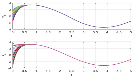
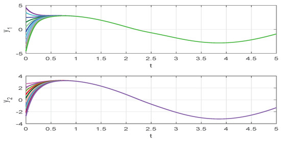
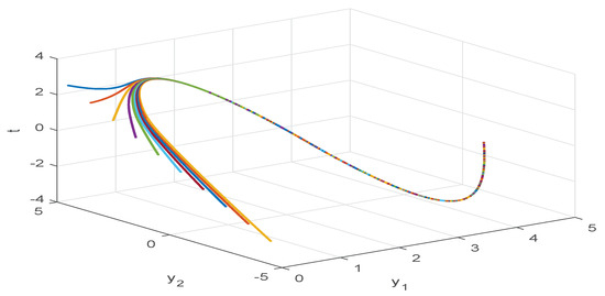
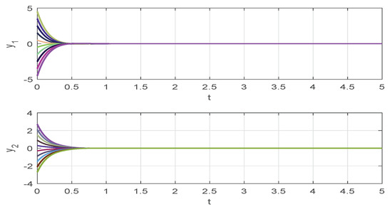
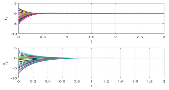
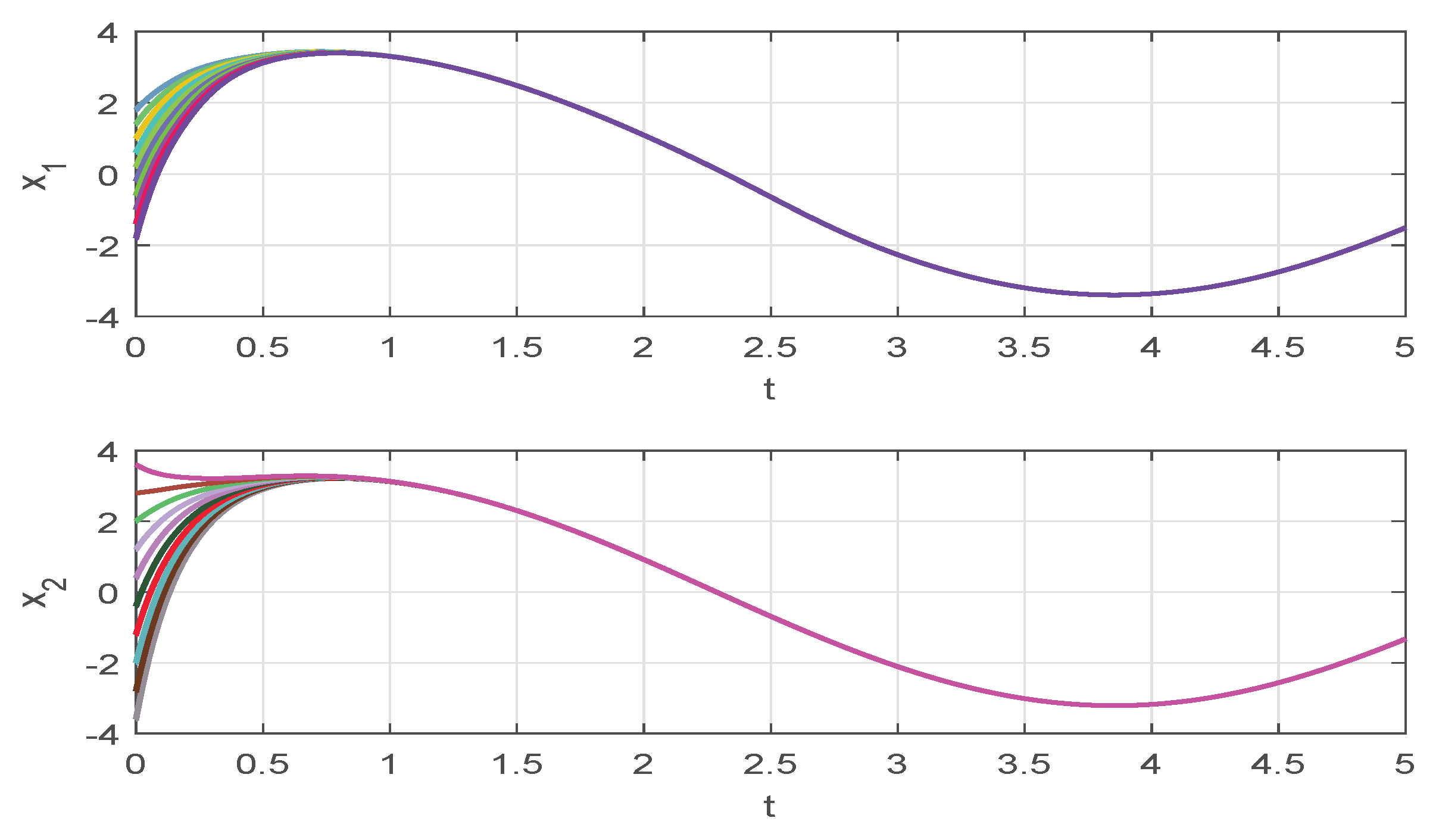
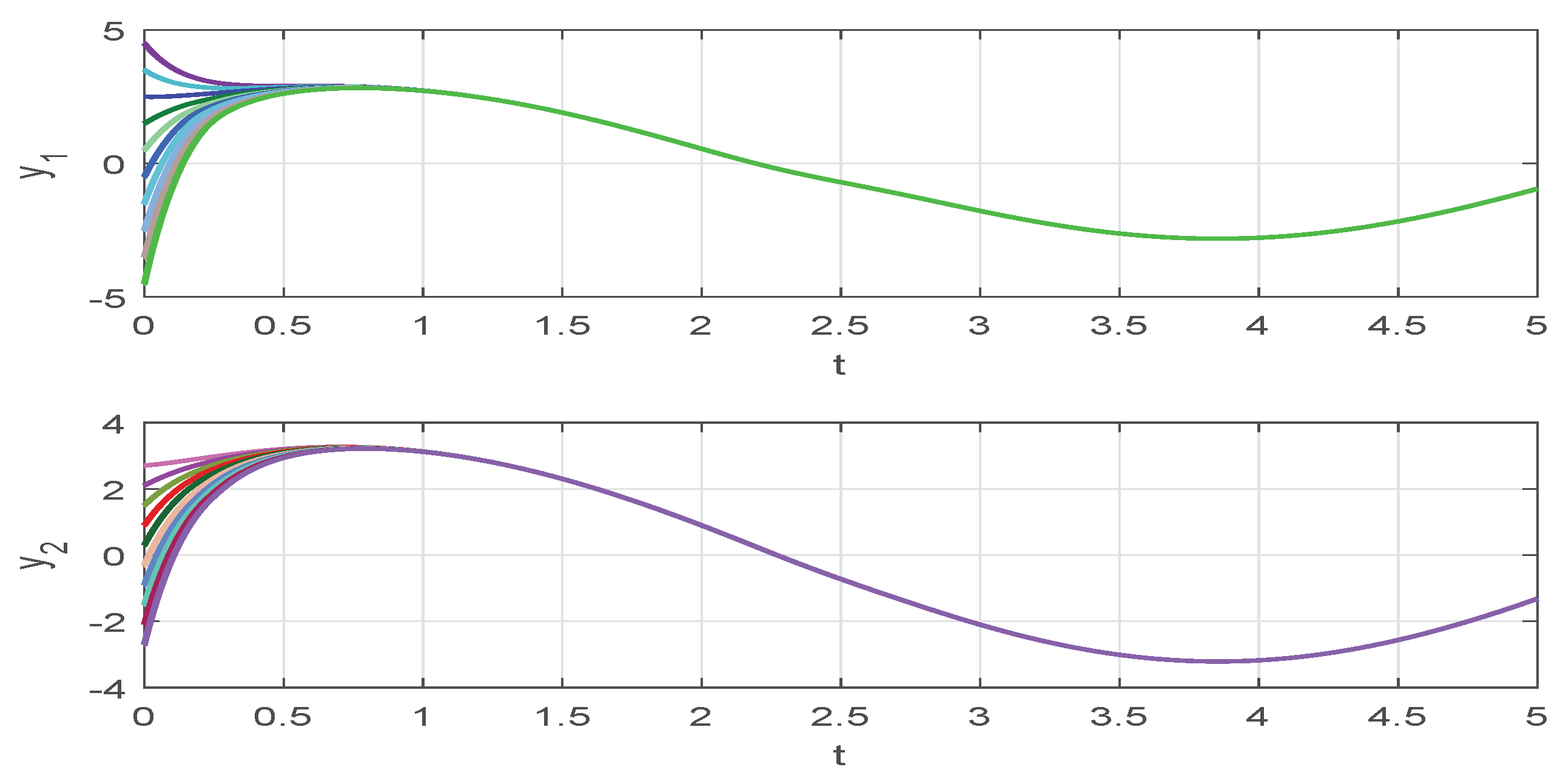
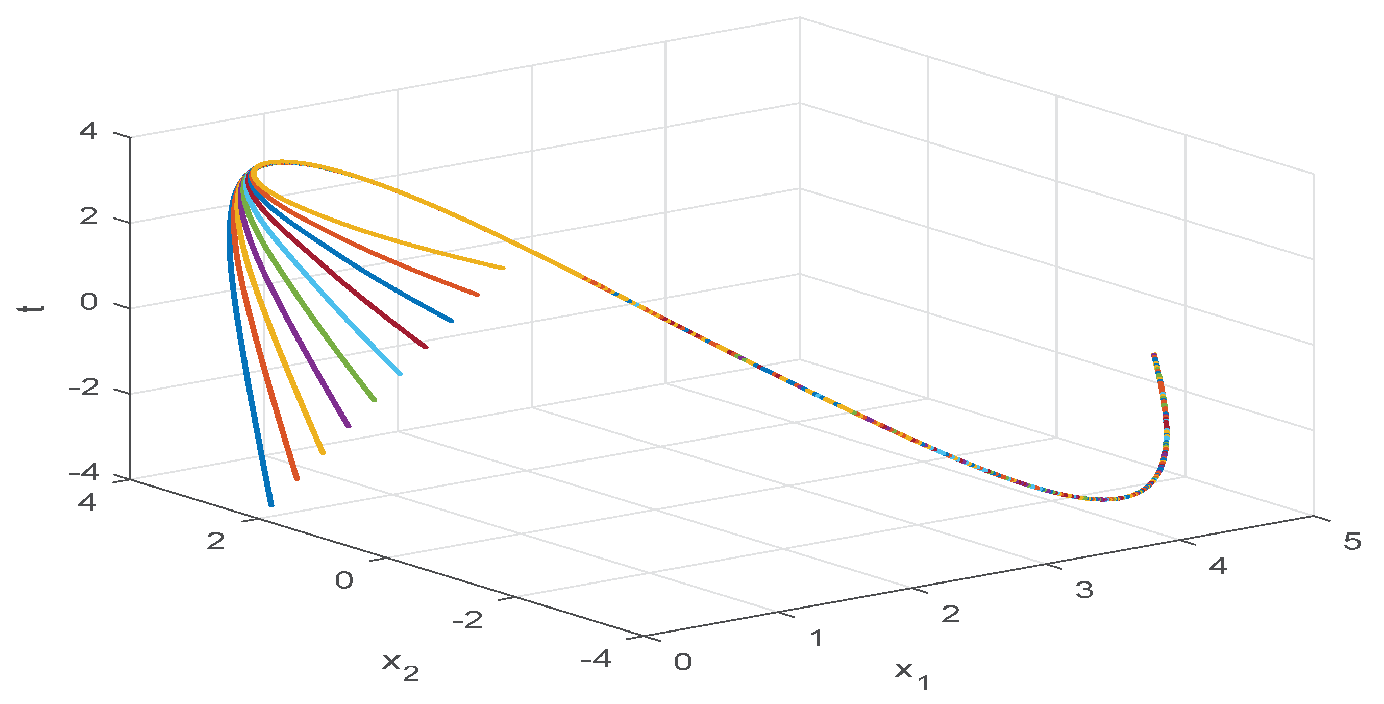
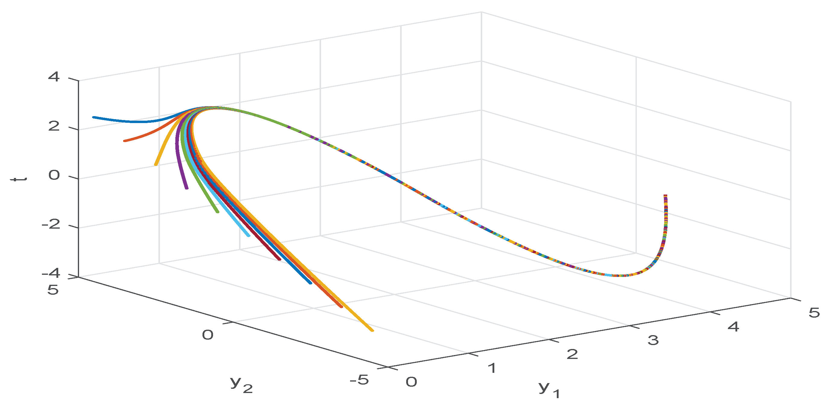
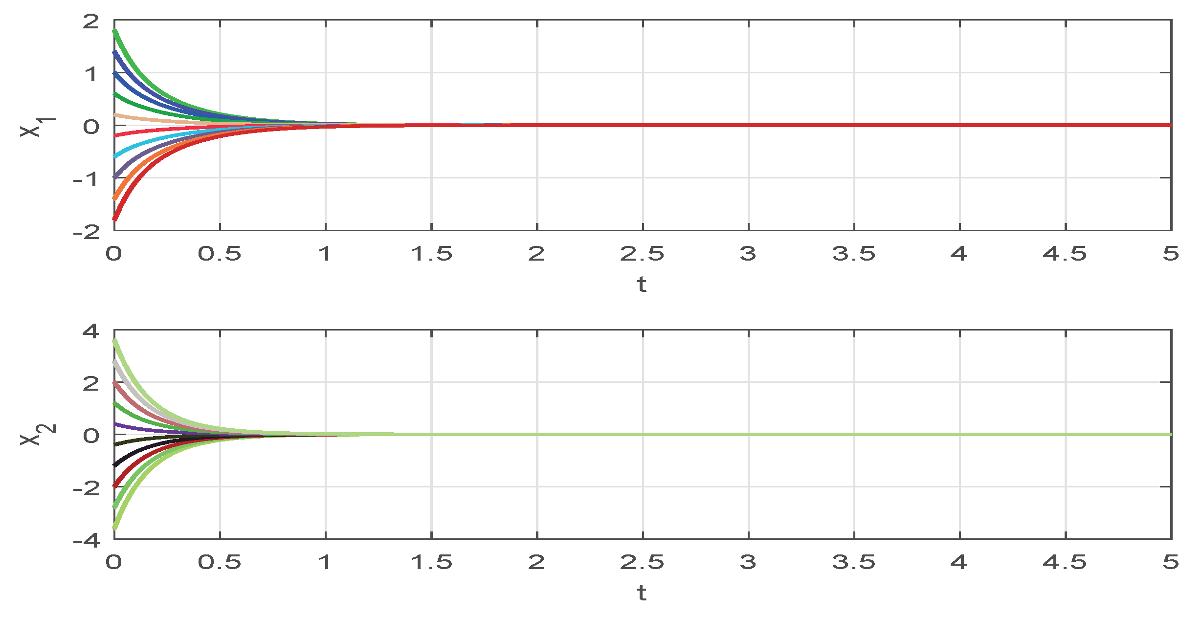
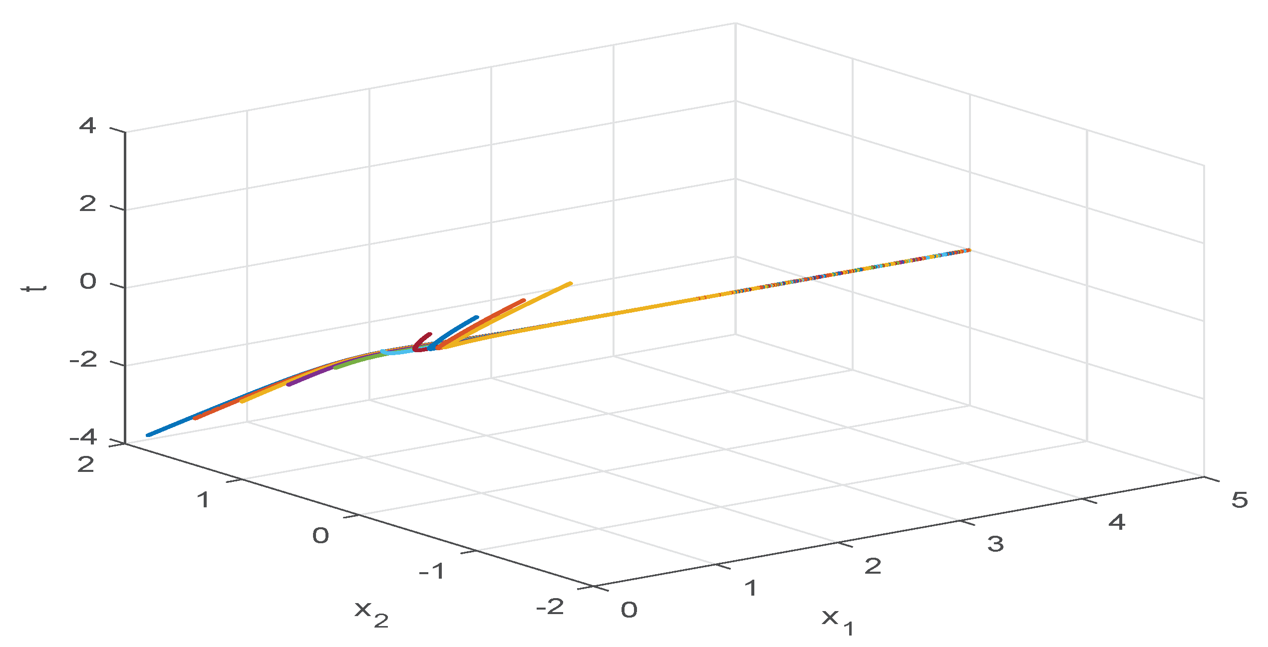
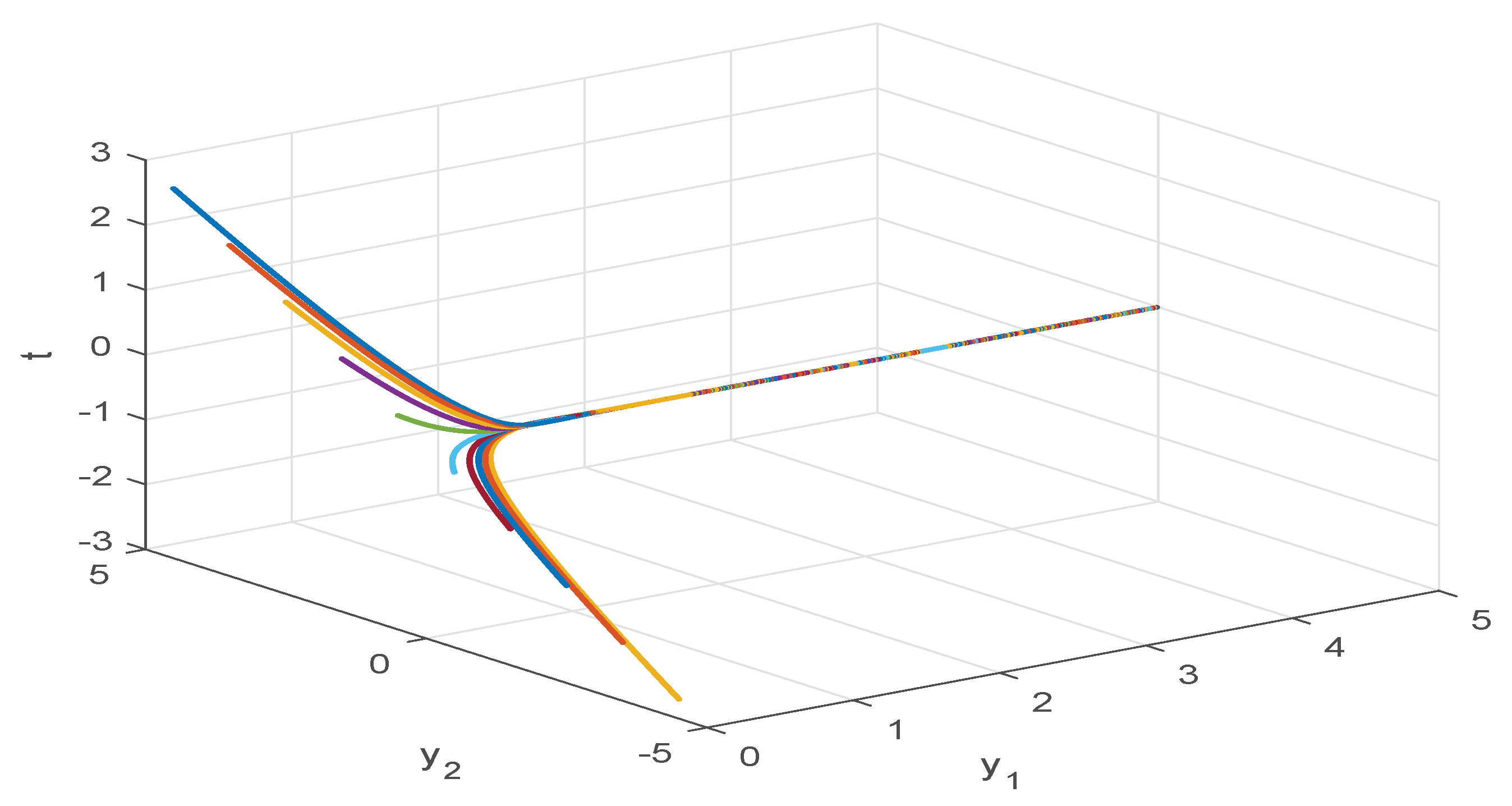
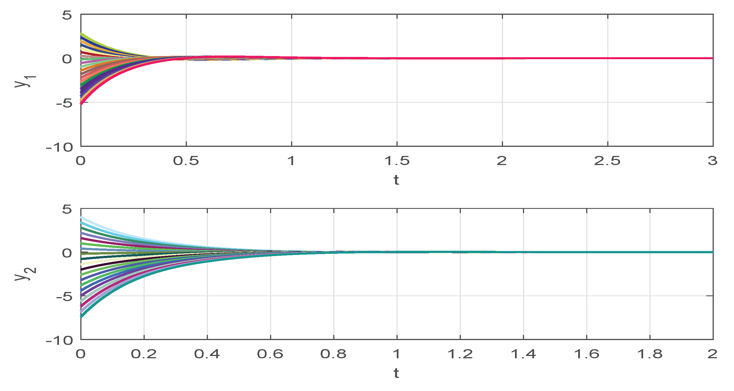
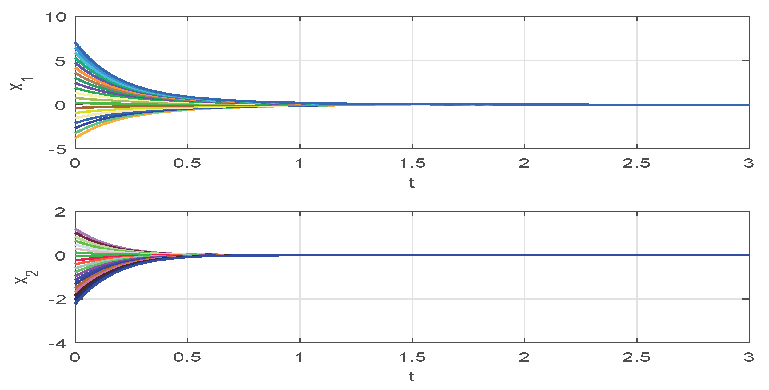
By using the MATLAB software package, the LMI (27) is true with $\mathfrak{n}=1,2,3$. With 10 randomly generated initial values, Figure 1, Figure 2, Figure 3 and Figure 4 depict the time response of the real and imaginary parts pertaining to the model in (20) with $\tilde{u}\left(t\right)=sin\left(0.02t\right)e^{-0.005t},t\ge 0$. When $\tilde{u}\left(t\right)=0$ and subject to the same initial conditions, the time responsed of the real and imaginary parts are shown in Figure 5, Figure 6, Figure 7 and Figure 8.

Figure 1. An illustration on the time responses with respect to the real parts pertaining to the model in (20), in which $\tilde{u}\left(t\right)=sin\left(0.02t\right)e^{-0.005t}$ in Example 1.

Figure 2. An illustration of the time responses with respect to the imaginary parts pertaining to the model in (20), in which $\tilde{u}\left(t\right)=sin\left(0.02t\right)e^{-0.005t}$ in Example 1.

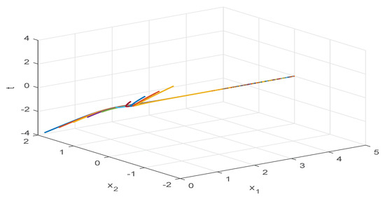
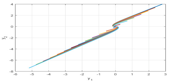
Figure 3. An illustration of the time responses between the real subspace pertaining to the model in (20), in which $\tilde{u}\left(t\right)=sin\left(0.02t\right)e^{-0.005t}$ in Example 1.

Figure 4. An illustration of the time responses between the imaginary subspace pertaining to the model in (20), in which $\tilde{u}\left(t\right)=sin\left(0.02t\right)e^{-0.005t}$ in Example 1.

Figure 5. An illustration of the time responses with respect to the real parts pertaining to the model in (20), in which $\tilde{u}\left(t\right)=0$ in Example 1.

Figure 6. An illustration of the time responses with respect to the imaginary parts pertaining to the model in (20), in which $\tilde{u}\left(t\right)=0$ in Example 1.

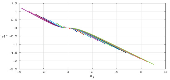
Figure 7. An illustration of the time responses between the real subspace pertaining to the model in (20), in which $\tilde{u}\left(t\right)=0$ in Example 1.

Figure 8. An illustration of the time responses between the imaginary subspace pertaining to the model in (20), in which $\tilde{u}\left(t\right)=0$ in Example 1.

Example 2.

The UHTCVNN model in (13) is considered, i.e.,

$$\begin{array}{cc}\mathcal{D}=\hfill & \left[\begin{array}{cc}3& 0\\ 0& 3\end{array}\right],\mathcal{A}=\left[\begin{array}{cc}1+i& -2+i\\ 1-i& -1+i\end{array}\right],\mathcal{G}=\left[\begin{array}{cc}0.1& 0\\ 0& 0.1\end{array}\right],{\mathcal{H}}_1=\left[\begin{array}{cc}0.2& 0\\ 0& 0.2\end{array}\right],\hfill \\ {\mathcal{H}}_2=\hfill & \left[\begin{array}{cc}0.2& 0\\ 0& 0.2\end{array}\right],{\mathcal{H}}_3=\left[\begin{array}{cc}0.1& 0\\ 0& 0.1\end{array}\right],\mathcal{J}=\left[\begin{array}{cc}0.3& 0\\ 0& 0.3\end{array}\right],\mathcal{L}=\left[\begin{array}{cc}\frac{1}{2}& 0\\ 0& \frac{1}{2}\end{array}\right],\mathcal{I}=\left[\begin{array}{cc}1& 0\\ 0& 1\end{array}\right]\hfill \end{array}$$

Take $\mathbf{Q},\mathbf{S},\mathbf{R}$ are the same as defined in Example 1, while ${\tilde{g}}_x\left({\tilde{\mathfrak{e}}}_x\right)=0.2\left(\right|{\tilde{\mathfrak{e}}}_x+1|-|{\tilde{\mathfrak{e}}}_x-1\left|\right),x=1,2.$ and $r\left(t\right)=0.2sint+0.6$ which satisfies $r=0.8$, $\mu =0.3$ and $\mathcal{F}\left(t\right)=0.2sint$.

Assume that ${\tilde{g}}_x\left(\tilde{\mathfrak{e}}\right)={\tilde{g}}_x^R(x,y)+i{\tilde{g}}_x^I(x,y),x=1,2$. By simple calculation, we have

$$\begin{array}{cc}\tilde{\mathcal{D}}=\hfill & \left[\begin{array}{cccc}3& 0& 0& 0\\ 0& 3& 0& 0\\ 0& 0& 3& 0\\ 0& 0& 0& 3\end{array}\right],\tilde{\mathcal{A}}=\left[\begin{array}{cccc}1& -2& -1& -1\\ 1& -1& 1& -1\\ 1& 1& 1& -2\\ -1& 1& 1& -1\end{array}\right],\tilde{\mathcal{G}}=\left[\begin{array}{cccc}0.1& 0& 0& 0\\ 0& 0.1& 0& 0\\ 0& 0& 0.1& 0\\ 0& 0& 0& 0.1\end{array}\right],\hfill \\ {\tilde{\mathcal{H}}}_1=\hfill & \left[\begin{array}{cccc}0.2& 0& 0& 0\\ 0& 0.2& 0& 0\\ 0& 0& 0.2& 0\\ 0& 0& 0& 0.2\end{array}\right],{\tilde{\mathcal{H}}}_2=\left[\begin{array}{cccc}0.2& 0& -0.1& 0\\ 0& 0.2& 0& -0.1\\ 0.1& 0& 0.2& 0\\ 0& 0.1& 0& 0.2\end{array}\right],\tilde{\mathcal{J}}=\left[\begin{array}{cccc}0.3& 0& 0& 0\\ 0& 0.3& 0& 0\\ 0& 0& 0.3& 0\\ 0& 0& 0& 0.3\end{array}\right],\hfill \\ \tilde{\mathcal{I}}=\hfill & \left[\begin{array}{cccc}1& 0& 0& 0\\ 0& 1& 0& 0\\ 0& 0& 1& 0\\ 0& 0& 0& 1\end{array}\right],\tilde{\mathcal{L}}=\left[\begin{array}{cccc}\frac{1}{2}& 0& 0& 0\\ 0& \frac{1}{2}& 0& 0\\ 0& 0& \frac{1}{2}& 0\\ 0& 0& 0& \frac{1}{2}\end{array}\right].\hfill \end{array}$$

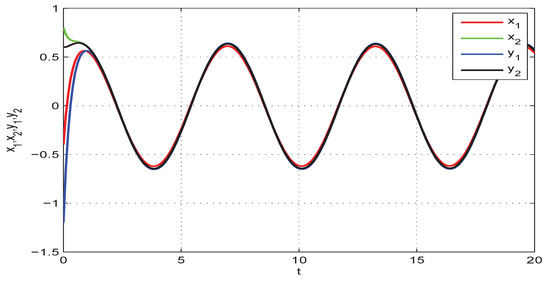
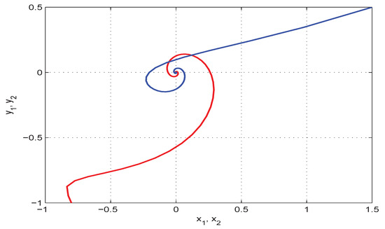
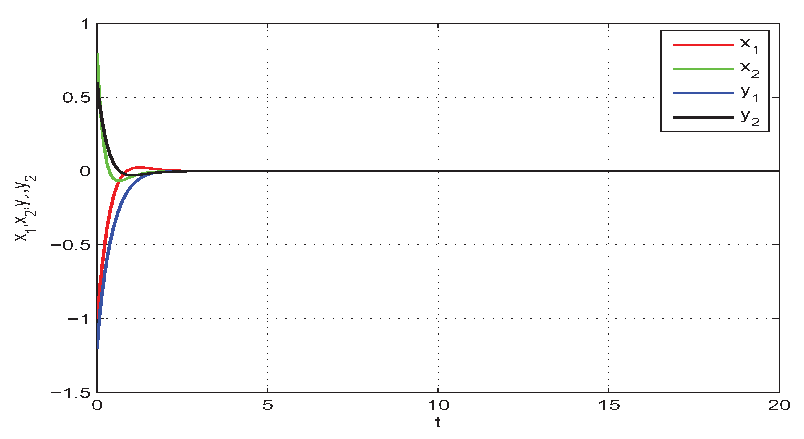
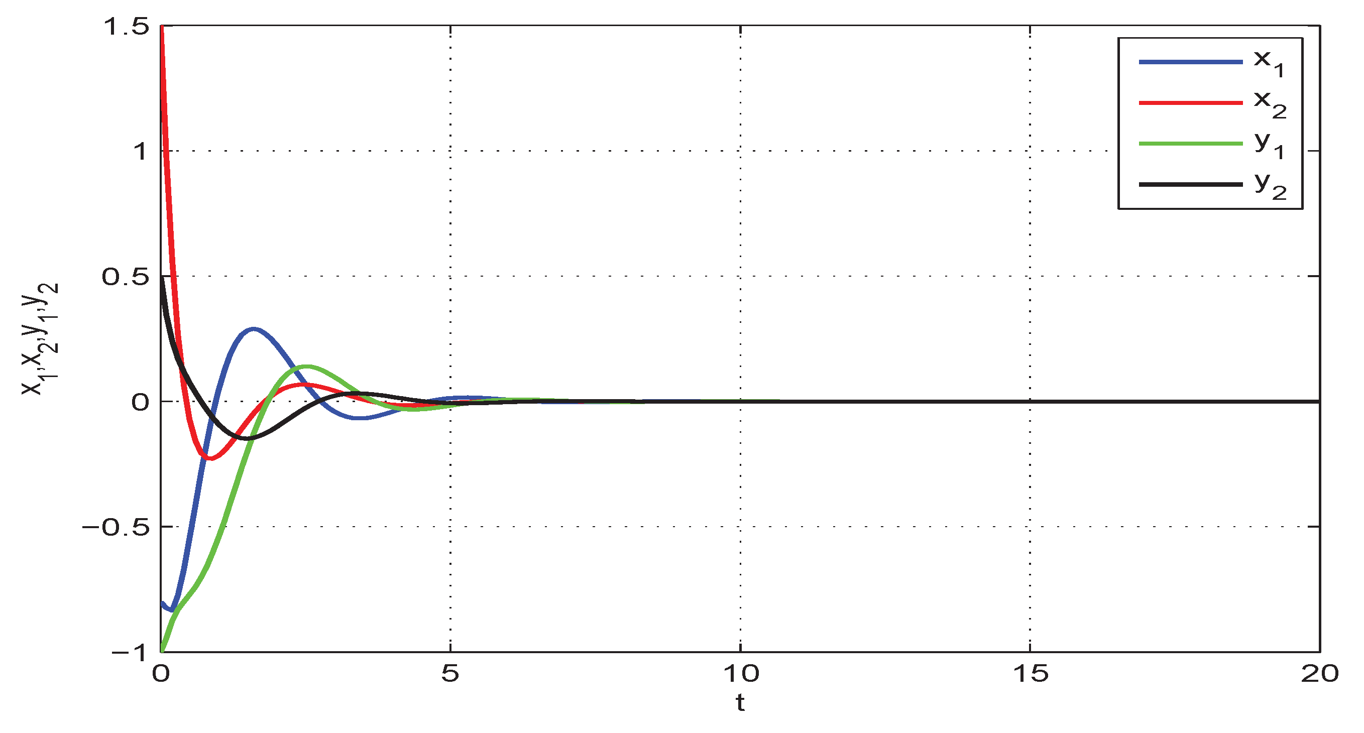
and $\tilde{\mathbf{Q}},\tilde{\mathbf{S}},\tilde{\mathbf{R}}$ are similar to those defined in Example 1. By using the MATLAB software package, the LMI (39) is satisfied with $\mathfrak{n}=1,2,3$. Subject to the initial values $\tilde{\mathfrak{e}}\left(0\right)={[-1,0.8,-1.2,0.6]}^T$, Figure 9 depict the time responses with respect to both the real and imaginary parts pertaining to the model in (13), in which $\tilde{u}\left(t\right)=sin\left(0.02t\right)e^{-0.005t},t\ge 0$. Based on the same initial conditions and with $\tilde{u}\left(t\right)=0$, the time responses with respect to both the real and imaginary parts of the model in (13) are shown in Figure 10.

Figure 9. An illustration of the time responses with respect to the real and imaginary parts of the states $p_1$ and $p_2$ pertaining to the model in (13) in a $2D$ space, in which $\tilde{u}\left(t\right)=sin\left(0.02t\right)e^{-0.005t}$ in Example 2.

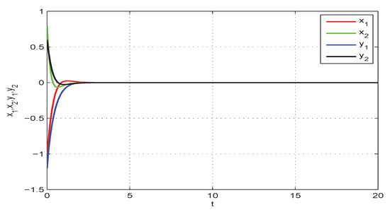
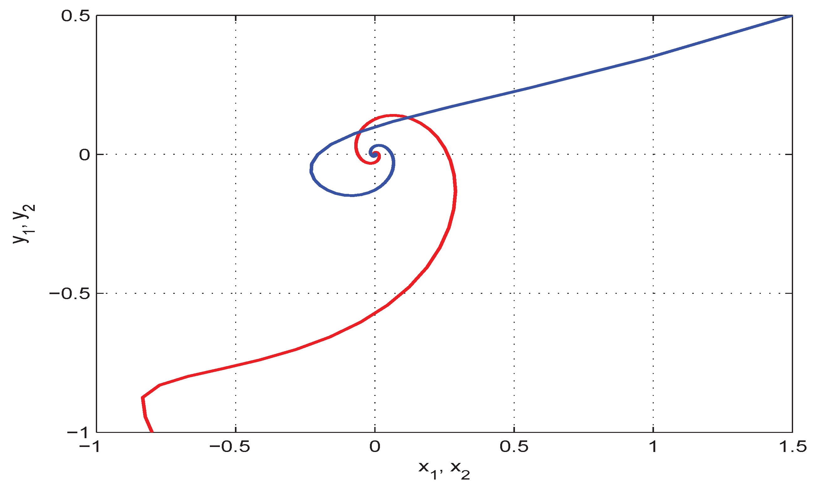
Figure 10. An illustration of the time responses with respect to the real and imaginary parts of the states $p_1$ and $p_2$ pertaining to the model in (13) in a $2D$ space, in which $\tilde{u}\left(t\right)=0$ in Example 2.

Example 3.

The HTCVNN model in (20) with $\tilde{u}\left(t\right)=0$ is considered, i.e.,

$$\begin{array}{cc}\frac{d}{dt}\tilde{\mathfrak{e}}\left(t\right)=\hfill & -\left[\begin{array}{cc}5& 0\\ 0& 5\end{array}\right]\tilde{\mathfrak{e}}\left(t\right)+\left[\begin{array}{cc}1+i& -2+i\\ 1-i& -1+0i\end{array}\right]\tilde{g}\left(\tilde{\mathfrak{e}}(t-r\left(t\right))\right).\hfill \end{array}$$

and $\mathcal{L}=\left[\begin{array}{cc}\frac{1}{2}& 0\\ 0& \frac{1}{2}\end{array}\right],{\tilde{g}}_x\left({\tilde{\mathfrak{e}}}_x\right)=0.5tanh\left({\tilde{\mathfrak{e}}}_x\right),x=1,2$.

Assume that ${\tilde{g}}_x\left(\tilde{\mathfrak{e}}\right)={\tilde{g}}_x^R(x,y)+i{\tilde{g}}_x^I(x,y),x=1,2$. It is straightforward to obtain

$$\begin{array}{c}\tilde{\mathcal{D}}=\left[\begin{array}{cccc}5& 0& 0& 0\\ 0& 5& 0& 0\\ 0& 0& 5& 0\\ 0& 0& 0& 5\end{array}\right],\tilde{\mathcal{A}}=\left[\begin{array}{cccc}1& -2& -1& -1\\ 1& -1& 1& 0\\ 1& 1& 1& -2\\ -1& 0& 1& -1\end{array}\right],\tilde{\mathcal{L}}=\left[\begin{array}{cccc}\frac{1}{4}& 0& 0& 0\\ 0& \frac{1}{4}& 0& 0\\ 0& 0& \frac{1}{4}& 0\\ 0& 0& 0& \frac{1}{4}\end{array}\right].\hfill \end{array}$$

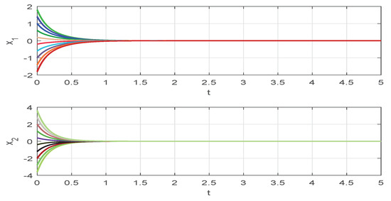
Take $r\left(t\right)=0.6+0.2sint$ which satisfies $r=0.8$ and $\mu =0.3$, and with the above parameters, we can use the MATLAB software package, the LMI (41) is true with $\mathfrak{n}=1,2,3$. Based on 20 randomly generated initial values, Figure 11, Figure 12, Figure 13 and Figure 14 depict the time responses with respect to both the imaginary and real parts pertaining to the model in (20). From the illustrations, we can confirm that the equilibrium point of the model in (20) is global asymptotic stable.

Figure 11. An illustration of the time responses with respect to the imaginary parts pertaining to the model in (20), in which $\tilde{u}\left(t\right)=0$ in Example 3.

Figure 12. An illustration of the time responses with respect to the real parts pertaining to the model in (20), in which $\tilde{u}\left(t\right)=0$ in Example 3.

Figure 13. An illustration of the time responses between the imaginary subspace pertaining to the model in (20), in which $\tilde{u}\left(t\right)=0$ in Example 3.

Figure 14. An illustration of the time responses between the real subspace pertaining to the model in (20), in which $\tilde{u}\left(t\right)=0$ in Example 3.

Example 4.

The CVHNN model in (13) with $\tilde{u}\left(t\right)=0$ is considered, i.e.,

$$\begin{array}{cc}\mathcal{D}=\hfill & \left[\begin{array}{cc}2& 0\\ 0& 2\end{array}\right],\mathcal{A}=\left[\begin{array}{cc}1+i& -2+i\\ 1-i& -1+0i\end{array}\right],\mathcal{G}=\left[\begin{array}{cc}0.1& 0\\ 0& 0.1\end{array}\right],{\mathcal{H}}_1=\left[\begin{array}{cc}0.2& 0\\ 0& 0.2\end{array}\right],\hfill \\ {\mathcal{H}}_2=\hfill & \left[\begin{array}{cc}0.2& 0\\ 0& 0.2\end{array}\right],{\mathcal{H}}_3=\left[\begin{array}{cc}0.1& 0\\ 0& 0.1\end{array}\right],\mathcal{J}=\left[\begin{array}{cc}0.3& 0\\ 0& 0.3\end{array}\right],\mathcal{L}=\left[\begin{array}{cc}\frac{1}{4}& 0\\ 0& \frac{1}{4}\end{array}\right],\hfill \\ {\tilde{g}}_x\left({\tilde{\mathfrak{e}}}_x\right)=\hfill & 0.5\left(\right|{\tilde{\mathfrak{e}}}_x+1|-|{\tilde{\mathfrak{e}}}_x-1\left|\right),x=1,2,\mathcal{F}\left(t\right)=0.2sint.\hfill \end{array}$$

Assume that ${\tilde{g}}_x\left(\tilde{\mathfrak{e}}\right)={\tilde{g}}_x^R(x,y)+i{\tilde{g}}_x^I(x,y),x=1,2$. By simple calculation, we have

$$\begin{array}{cc}\hfill & \tilde{\mathcal{D}}=\left[\begin{array}{cccc}2& 0& 0& 0\\ 0& 2& 0& 0\\ 0& 0& 2& 0\\ 0& 0& 0& 2\end{array}\right],\tilde{\mathcal{A}}=\left[\begin{array}{cccc}1& -2& -1& -1\\ 1& -1& 1& 0\\ 1& 1& 1& -2\\ -1& 0& 1& -1\end{array}\right],\tilde{\mathcal{G}}=\left[\begin{array}{cccc}0.1& 0& 0& 0\\ 0& 0.1& 0& 0\\ 0& 0& 0.1& 0\\ 0& 0& 0& 0.1\end{array}\right],\hfill \\ \hfill & {\tilde{\mathcal{H}}}_1=\left[\begin{array}{cccc}0.2& 0& 0& 0\\ 0& 0.2& 0& 0\\ 0& 0& 0.2& 0\\ 0& 0& 0& 0.2\end{array}\right],{\tilde{\mathcal{H}}}_2=\left[\begin{array}{cccc}0.2& 0& -0.1& 0\\ 0& 0.2& 0& -0.1\\ 0.1& 0& 0.2& 0\\ 0& 0.1& 0& 0.2\end{array}\right],\tilde{\mathcal{J}}=\left[\begin{array}{cccc}0.3& 0& 0& 0\\ 0& 0.3& 0& 0\\ 0& 0& 0.3& 0\\ 0& 0& 0& 0.3\end{array}\right].\hfill \end{array}$$

$\tilde{\mathcal{L}}=diag\{0.5,0.5,0.5,0.5\}$. Take $r\left(t\right)=0.6+0.2sint$ which satisfies $r=0.8$ and $\mu =0.3$, and with the above parameters, we can use the MATLAB, the LMI (43) is true with $\mathfrak{n}=1,2,3$. We obtain the following results with the initial condition $\tilde{\mathfrak{e}}\left(0\right)={[-0.8,1.5,-1,0.5]}^T$. The time responses pertaining to the model in (13) with $\tilde{u}\left(t\right)=0$ are depicted in Figure 15 and Figure 16. According to Corollary 2, we can confirm that the equilibrium point of the model in (5) or the equivalent real-valued model in (13) is global asymptotic stable.

Figure 15. An illustration of the time responses with respect to both the real and imaginary parts of the states $p_1$ and $p_2$ pertaining to the model in (13) in a $2D$ space, in which $\tilde{u}\left(t\right)=0$ in Example 4.

Figure 16. An illustration of the time responses between the real and imaginary subspace pertaining to the model in (13), in which $\tilde{u}\left(t\right)=0$ in Example 4.

5. Conclusions

An investigation on the robust dissipativity with respect to the HTCVNN models with linear fractional uncertainties and time-varying delays was conducted. To facilitate the analysis, we devised an appropriate LKF with general integral terms and employed the multiple integral inequality method to yield the sufficient conditions of dissipativity with respect to the HTCVNN models in the form of LMIs. The MATLAB software package was used to solve the LMIs effectively. We also illustrated the feasibility of the results through several numerical models and their simulation results. Note that the features of HTCVNNs are closely connected with other CVNN models. As a result, we intend to extend the obtained results to study various dynamical behaviours of different fractional-order CVNN models in our future research.

References

- Wang, Z.; Guo, Z.; Huang, L.; Liu, X. Dynamical behavior of complex-valued Hopfield neural networks with discontinuous activation functions. Neural Process. Lett. 2017, 45, 1039–1061. [Google Scholar] [CrossRef]
- Song, Q.; Zhao, Z.; Liu, Y. Stability analysis of complex-valued neural networks with probabilistic time-varying delays. Neurocomputing 2015, 159, 96–104. [Google Scholar] [CrossRef]
- Sriraman, R.; Cao, Y.; Samidurai, R. Global asymptotic stability of stochastic complex-valued neural networks with probabilistic time-varying delays. Math. Comput. Simul. 2020, 171, 103–118. [Google Scholar] [CrossRef]
- Chen, X.; Song, Q. Global stability of complex-valued neural networks with both leakage time delay and discrete time delay on time scales. Neurocomputing 2013, 121, 254–264. [Google Scholar] [CrossRef]
- Pratap, A.; Raja, R.; Cao, J.; Rajchakit, G.; Lim, C.P. Global robust synchronization of fractional order complex-valued neural networks with mixed time varying delays and impulses. Int. J. Control Autom. Syst. 2019, 17, 509–520. [Google Scholar]
- Gong, W.; Liang, J.; Kan, X.; Nie, X. Robust state estimation for delayed complex-valued neural networks. Neural Process. Lett. 2017, 46, 1009–1029. [Google Scholar] [CrossRef]
- Samidurai, R.; Sriraman, R.; Zhu, S. Leakage delay-dependent stability analysis for complex-valued neural networks with discrete and distributed time-varying delays. Neurocomputing 2019, 338, 262–273. [Google Scholar] [CrossRef]
- Samidurai, R.; Sriraman, R.; Cao, J.; Tu, Z. Effects of leakage delay on global asymptotic stability of complex-valued neural networks with interval time-varying delays via new complex-valued Jensen’s inequality. Int. J. Adapt. Control Signal Process. 2018, 32, 1294–1312. [Google Scholar] [CrossRef]
- Wang, Z.; Huang, L. Global stability analysis for delayed complex-valued BAM neural networks. Neurocomputing 2016, 173, 2083–2089. [Google Scholar] [CrossRef]
- Subramanian, K.; Muthukumar, P. Global asymptotic stability of complex-valued neural networks with additive time-varying delays. Cogn. Neurodyn. 2017, 11, 293–306. [Google Scholar] [CrossRef]
- Zhang, Z.; Liu, X.; Guo, R.; Lin, C. Finite-time stability for delayed complex-valued BAM neural networks. Neural Process. Lett. 2018, 48, 179–193. [Google Scholar] [CrossRef]
- Zhang, Z.; Liu, X.; Zhou, D.; Lin, C.; Chen, J.; Wang, H. Finite-time stabilizability and instabilizability for complex-valued memristive neural networks with time delays. IEEE Trans. Syst. Man Cybern. Syst. 2018, 48, 2371–2382. [Google Scholar] [CrossRef]
- Mishra, D.; Tolambiya, A.; Shukla, A.; Kalra, P. Stability analysis for higher order complex-valued Hopfield neural network. Neural Inf. Process. 2006, 4232, 608–615. [Google Scholar]
- Liu, D.; Zhu, S.; Ye, E. Synchronization stability of memristor-based complex-valued neural networks with time delays. Neural Netw. 2017, 96, 115–127. [Google Scholar] [CrossRef] [PubMed]
- Liu, D.; Zhu, S.; Chang, W. Mean square exponential input-to-state stability of stochastic memristive complex-valued neural networks with time varying delay. Int. J. Syst. Sci. 2017, 48, 1966–1977. [Google Scholar] [CrossRef]
- Li, X.; Ding, D. Mean square exponential stability of stochastic Hopfield neural networks with mixed delays. Stat. Probab. Lett. 2017, 126, 88–96. [Google Scholar] [CrossRef]
- Wang, T.; Zhao, S.; Zhou, W.; Yu, W. Finite-time state estimation for delayed Hopfield neural networks with Markovian jump. Neurocomputing 2015, 156, 193–198. [Google Scholar] [CrossRef]
- Liu, L.; Deng, F. Stability analysis of time varying delayed stochastic Hopfield neural networks in numerical simulation. Neurocomputing 2018, 316, 294–305. [Google Scholar] [CrossRef]
- Park, M.J.; Kwon, O.M.; Ryu, J.H. Generalized integral inequality: Application to time-delay systems. Appl. Math. Lett. 2018, 77, 6–12. [Google Scholar] [CrossRef]
- Chen, J.; Xu, S.; Chen, W.; Zhang, B.; Ma, Q.; Zou, Y. Two general integral inequalities and their applications to stability analysis for systems with time-varying delay. Int. J. Robust Nonlinear Control 2016, 26, 4088–4103. [Google Scholar] [CrossRef]
- Wang, J.; Wang, Z.; Ding, S.; Zhang, H. Refined Jensen-based multiple integral inequality and its application to stability of time-delay systems. IEEE/CAA J. Automat. Sinica 2018, 5, 758–764. [Google Scholar] [CrossRef]
- Kwon, O.M.; Park, M.J.; Park, J.H.; Lee, S.M.; Cha, E.J. Analysis on robust H∞ performance and stability for linear systems with interval time-varying state delays via some new augmented Lyapunov-Krasovskii functional. Appl. Math. Comput. 2013, 224, 108–122. [Google Scholar]
- Li, T.; Guo, L.; Sun, C. Robust stability for neural networks with time-varying delays and linear fractional uncertainties. Neurocomputing 2007, 71, 421–427. [Google Scholar] [CrossRef]
- Sakthivel, R.; Shi, P.; Arunkumar, A.; Mathiyalagan, K. Robust reliable H∞ control for fuzzy systems with random delays and linear fractional uncertainties. Fuzzy Set. Syst. 2016, 302, 65–81. [Google Scholar] [CrossRef]
- Samidurai, R.; Sriraman, R. Robust dissipativity analysis for uncertain neural networks with additive time-varying delays and general activation functions. Math. Comput. Simul. 2019, 155, 201–216. [Google Scholar] [CrossRef]
- Mahmoud, M.S.; Saif, A.W.A. Dissipativity analysis and design for uncertain Markovian jump systems with time-varying delays. Appl. Math. Comput. 2013, 219, 9681–9695. [Google Scholar] [CrossRef]
- Wu, Z.G.; Lam, J.; Su, H.; Chu, J. Stability and dissipativity analysis of static neural networks with time delay. IEEE Trans. Neural Netw. Learn. Syst. 2012, 23, 199–210. [Google Scholar]
- Feng, Z.; Lam, J. Stability and dissipativity analysis of distributed delay cellular neural networks. IEEE Trans. Neural Netw. 2011, 22, 976–981. [Google Scholar] [CrossRef]
- Raja, R.; Raja, U.K.; Samidurai, R.; Leelamani, A. Dissipativity of discrete-time BAM stochastic neural networks with Markovian switching and impulses. J. Frankl. Inst. 2013, 350, 3217–3247. [Google Scholar] [CrossRef]
- Zeng, H.B.; Park, J.H.; Zhang, C.F.; Wang, W. Stability and dissipativity analysis of static neural networks with interval time-varying delay. J. Frankl. Inst. 2015, 352, 1284–1295. [Google Scholar] [CrossRef]
- Li, X.; Rakkiyappan, R.; Velmurugan, G. Dissipativity analysis of memristor-based complex-valued neural networks with time-varying delays. Inform. Sci. 2015, 294, 645–665. [Google Scholar] [CrossRef]
- Rajivganthi, C.; Rihan, F.A.; Lakshmanan, S. Dissipativity analysis of complex-valued BAM neural networks with time delay. Neural Comput. Appl. 2019, 31, 127–137. [Google Scholar] [CrossRef]
- Rakkiyappan, R.; Velmurugan, G.; Li, X.; Regan, D.O. Global dissipativity of memristor-based complex-valued neural networks with time-varying delays. Neural Comput. Appl. 2016, 27, 629–649. [Google Scholar] [CrossRef]
- Ramasamy, S.; Nagamani, G. Dissipativity and passivity analysis for discrete-time complex-valued neural networks with leakage delay and probabilistic time-varying delays. Int. J. Adapt. Control Signal Process. 2017, 31, 876–902. [Google Scholar] [CrossRef]
- Nagamani, G.; Ramasamy, S. Dissipativity and passivity analysis for discrete-time complex-valued neural networks with time-varying delays. Cogent Math. 2015, 2, 1048580. [Google Scholar] [CrossRef]
- Cao, Y.; Sriraman, R.; Shyamsundarraj, N.; Samidurai, R. Robust stability of uncertain stochastic complex-valued neural networks with additive time-varying delays. Math. Comput. Simul. 2020, 171, 207–220. [Google Scholar] [CrossRef]
- Liu, M.; Wang, X.; Zhang, Z.; Wang, Z. Dissipativity analysis of complex-valued stochastic neural networks with time-varying delays. IEEE Access 2019, 7, 165076–165087. [Google Scholar] [CrossRef]
- Cao, Y.; Samidurai, R.; Sriraman, R. Stability and stabilization analysis of nonlinear time-delay systems with randomly occurring controller gain fluctuation. Math. Comput. Simul. 2020, 171, 36–51. [Google Scholar] [CrossRef]
- Subramanian, K.; Muthukumar, P.; Lakshmanan, S. State feedback synchronization control of impulsive neural networks with mixed delays and linear fractional uncertainties. Appl. Math. Comput. 2018, 321, 267–281. [Google Scholar] [CrossRef]
- Hill, D.L.; Moylan, P.J. Dissipative dynamical systems: Basic input-output and state properties. J. Frankl. Inst. 1980, 309, 327–357. [Google Scholar] [CrossRef]
© 2020 by the authors. Licensee MDPI, Basel, Switzerland. This article is an open access article distributed under the terms and conditions of the Creative Commons Attribution (CC BY) license (http://creativecommons.org/licenses/by/4.0/).