Article

Powers of the Stochastic Gompertz and Lognormal Diffusion Processes, Statistical Inference and Simulation

by
Eva María Ramos-Ábalos
1,*,†,
Ramón Gutiérrez-Sánchez
1,† and
Ahmed Nafidi
2,†
1
Department of Statistics and Operational Research, Faculty of Science, University of Granada, Avda. Fuentenueva, S/N, 18071 Granada, Spain
2
Department of Mathematics and Informatics, LAMSAD, National School of Applied Sciences Berrechid, University of Hassan 1, Avenue de l’université, BP 280 Berrechid, Morocco
*
Author to whom correspondence should be addressed.
These authors contributed equally to this work.
Mathematics 2020, 8(4), 588; https://doi.org/10.3390/math8040588
Submission received: 5 March 2020 / Revised: 10 April 2020 / Accepted: 13 April 2020 / Published: 15 April 2020

Abstract

:
In this paper, we study a new family of Gompertz processes, defined by the power of the homogeneous Gompertz diffusion process, which we term the powers of the stochastic Gompertz diffusion process. First, we show that this homogenous Gompertz diffusion process is stable, by power transformation, and determine the probabilistic characteristics of the process, i.e., its analytic expression, the transition probability density function and the trend functions. We then study the statistical inference in this process. The parameters present in the model are studied by using the maximum likelihood estimation method, based on discrete sampling, thus obtaining the expression of the likelihood estimators and their ergodic properties. We then obtain the power process of the stochastic lognormal diffusion as the limit of the Gompertz process being studied and go on to obtain all the probabilistic characteristics and the statistical inference. Finally, the proposed model is applied to simulated data.

1. Introduction

Stochastic processes are used to model stochastic phenomena in various fields of science, engineering, economics and finance. An important category among these processes is that of Stochastic Diffusion Processes (SDP), which have received considerable attention recently, due on the one hand to their diverse applications in stochastic modelling, and on the other, to their value in addressing probabilistic statistical problems, especially those involving statistical inference. In consequence, these processes have been widely studied, and much research has been undertaken to resolve these issues of statistical inference, with particular respect to the estimation of parameters; see, among others, Bibby and Sorensen [1], Prakasa Rao [2], Chang and Cheng [3], Beskos et al. [4], Stramer and Yan [5], Shoji and Ozaki [6], Durham and Gallant [7] and Fan [8], without forgetting the works of Yenkie and Diwekar [9] and Kloeden et al. [10] and the important bibliography cited in these works.
There has been much recent interest in applying SDP, and many researchers are working on the construction of stochastic processes in order to model phenomena of interest. These processes are used in areas such as the stochastic economy, new technologies, interest rates, courses of action, insurance, finance in general, cell growth, radiotherapy, chemotherapy, emissions from energy consumption and the emissions of CO 2 and greenhouse gases. Research results have been applied to various processes, both in the homogeneous and in the non-homogeneous cases and many particular SDP have been proposed, such as Katsamaki and Skiadas [11] in the case of the exponential model, Skiadas and Giovanis [12] in the case of the Bass model, Giovanis and Skiadas [13] in the case of the logistic model, Gutiérrez et al. [14] in the case of the Rayleigh model and Román-Román et al. [15] in the case of the lognormal with exogenous factors.
Among the above-mentioned processes is the Stochastic Gompertz Diffusion Process (SGDP), which was first proposed by Ricciardi [16], who defined it in the homogeneous case by means of stochastic differential equations, for use in studies of population growth. It was subsequently used by Dennis and Patil [17] in ecology modelling. With respect to the Kolmogorov equations, it was defined by Nafidi [18], in a general way and for both the univariate and the multivariate cases.
In various papers, Gutiérrez et al. [19,20,21], Ferrante et al. [22], Román-Román et al. [23] and Giorno and Nobile [24], have highlighted the importance of this process, and many subsequent extensions have appeared, especially regarding the non-homogeneous case with exogenous factors (external variables) that affect the drift coefficient. In general, these extensions take one of the following two forms:
With external information (when no functional form is available): the exogenous factors are completely determined by the observed data (monthly, annual, etc.) and to obtain their functional forms interpolation methods, among others, can be used. This methodology has been applied by Gutiérrez et al. [25,26], Rupsys et al. [27] and Badurally Adam et al. [28]. In all these papers it is assumed that the coefficient drift is a linear combination of exogenous factors, obtained by linear interpolation.
Without external information: in this case there are no observed data for the exogenous factors, but they are functions of time and of certain parameters. For example, the case in which the deceleration factor is affected by exogenous factors was developed by Gutiérrez et al. [29]. Ferrante et al. [30] studied the Gompertz process in which exogenous factors are obtained as the sum of two exponential functions and Albano and Giorno [31] did so considering logarithmic exogenous factor.
The lognormal SDP and the SGDP, in turn, have been extended to the multivariate case with delay, by Frank [32], and to the bivariate case without delay by Gutiérrez et al. [33], and an application has been devised to model the emissions of CO 2 in Spain [34]. Other recent papers that have addressed questions related to SGDP include Hu [35] and Zou et al. [36].
In the present study, we define and examine a new extension of the Gompertz and lognormal diffusion processes, based on the homogeneous version of these processes, i.e., their power. Thus, we obtain two families of homogeneous diffusion processes. Firstly, we show that Gompertzian and lognormal diffusions are stable by power transformation. Them we define the proposed model as the solution to a stochastic differential equation. From this, we obtain: the explicit expression of the process, the Probability Transition Density Function (PTDF), the moments of different orders and, in particular, the conditioned and unconditioned trends of the process; the ergodicity of the process and its stationary distribution and the process parameters, estimated by maximum likelihood, with discrete sampling, determining the asymptotic properties of the likelihood estimators and the approximated confidence interval of the parameters.
In addition, we obtain the probabilistic and statistical characteristics of the lognormal process power, as a particular case of the process being studied, when the deceleration factor tends toward zero. Finally, the process and the methodology presented are applied to simulated data obtained from the explicit expression of the solution to the characteristic state equation for the process.

2. The Model and Its Basic Probabilistic Characteristics

2.1. An Overview of the Homogeneous Gompertz Stochastic Diffusion Process

Let X ( t ) ; t [ t 0 , T ] ; t 0 0 be a stochastic process taking values on ( 0 , ) , X ( t ) is a Gompertz diffusion process with parameters α , β and σ and which is denoted by Gomp ( α ; β ; σ ) if X ( t ) satisfies Ito’s Stochastic Differential Equation (SDE) as follows (see [16,18,20,37]):
d X ( t ) = α X ( t ) β X ( t ) log X ( t ) d t + σ X ( t ) d w t ; P ( X ( t 0 ) = X t 0 ) = 1
In the literature, the constant α ( R ) is the intrinsic growth rate; the β ( R ) constant is the deceleration factor, the σ > 0 constant is the diffusion coefficient, X t 0 > 0 is a fixed real number and w t denotes the one-dimensional standard Wiener process.
The analytical expression of the unique solution to Equation (1) is given by (see, for example, [21,37])
X ( t ) = exp e β ( t t 0 ) log X t 0 + α σ 2 / 2 β 1 e β ( t t 0 ) + σ t 0 t e β ( t τ ) d w ( τ )
From this, we deduce that the process X ( t ) is distributed as the following one-dimensional lognormal distribution:
Λ 1 e β ( t t 0 ) log X t 0 + ( α σ 2 / 2 ) β 1 e β ( t t 0 ) ; σ 2 2 β 1 e 2 β ( t t 0 )
It has been shown (see [21]), that for β > 0 , X ( t ) is ergodic and that the stationary distribution has a lognormal distribution. Hence, we have:
X ( ) Λ 1 α σ 2 / 2 β ; σ 2 2 β

2.2. The Proposed Model

Let X ( t ) ; t [ t 0 , T ] ; t 0 0 be a Gomp ( α ; β ; σ ) . Then, the γ -power of the Stochastic Gompertz Diffusion Process ( γ -PSGDP) X ( t ) is defined by
x γ ( t ) = X γ ( t ) ; γ R *
The process x γ ( t ) ; t [ t 0 , T ] ; t 0 0 is also a diffusion process with values in ( 0 , ) and has the drift and diffusion coefficients are shown below.
By applying Ito’s formula to the transform given in Equation (4), we have
d x γ ( t ) = γ X γ 1 ( t ) α X ( t ) β X ( t ) log X ( t ) d t + γ σ X γ ( t ) d W t + γ ( γ 1 ) σ 2 2 X γ ( t ) d t   = α γ X γ ( t ) β γ X γ ( t ) log X ( t ) d t + γ σ X γ ( t ) d W t
Then, after some algebraic rearrangement, we obtain
d x γ ( t ) = a x γ ( t ) β x γ ( t ) log x γ ( t ) d t + c x γ ( t ) d w ( t )
This shows that the process x γ ( t ) is also a Gomp ( a ; β ; c ) process, where:
a = γ α + γ ( γ 1 ) σ 2 2   and   c = γ σ and the drift and diffusion coefficients are given respectively by:
A 1 ( x ) = γ α + γ ( γ 1 ) ) σ 2 2 x β x log ( x ) A 2 ( x ) = γ 2 σ 2 x 2
The model proposed in this paper belongs to the family of processes γ -PSGDP x γ ( t ) ; t [ t 0 , T ] ; t 0 0 defined by the following SDE:
d x γ ( t ) = A 1 ( x γ ( t ) ) d t + A 2 ( x γ ( t ) ) d w ( t ) ; P ( x γ ( t 0 ) = x t 0 ) = 1

2.3. Probabilistic Characteristics of the γ -PSGDP

Under the initial condition given, the unique solution of the SDE Equation (5) can be obtained using the relations expressed by Equations (2) and (4), from which we have
x γ ( t ) = exp e β ( t t 0 ) log x t 0 + γ ( α σ 2 / 2 ) β 1 e β ( t t 0 ) + γ σ t 0 t e β ( t τ ) d w ( τ )
We then deduce that x γ ( t ) is distributed as a one dimensional lognormal distribution Λ 1 ( μ ( s , t , x t 0 ) , γ 2 σ 2 λ 2 ( t 0 , t ) ) , where μ ( s , t , x t 0 ) and λ 2 ( t 0 , t ) are given by
μ ( s , t , x t 0 ) = e β ( t t 0 ) log x t 0 + γ ( α σ 2 / 2 ) β 1 e β ( t t 0 ) λ 2 ( t 0 , t ) = 1 2 β 1 e 2 β ( t t 0 )
From the homogeneity of the process, we know that x γ ( t ) x γ ( s ) = x s has the lognormal distribution Λ 1 ( μ ( s , t , x s ) , σ 2 λ 2 ( s , t ) ) , and then the PTDF of the process is
f ( y , t x , s ) = 1 y 2 π γ 2 σ 2 λ 2 ( s , t ) 1 / 2 exp log ( y ) μ ( s , t , x ) 2 2 γ 2 σ 2 λ 2 ( s , t )
The rth conditional moment of the process is given by
E x γ r ( t ) x γ ( s ) = x s = exp r μ ( s , t , x s ) + r 2 γ 2 σ 2 2 λ 2 ( s , t )
from which the Conditional Trend Function (CTF) gives
E x γ ( t ) x γ ( s ) = x s = exp e β ( t s ) log x s + γ ( α σ 2 / 2 ) β 1 e β ( t s )     + γ 2 σ 2 4 β 1 e 2 β ( t s )
Assuming the initial condition P ( x γ ( t 0 ) = x t 0 ) = 1 , the Trend Function (TF) of the process is
E x γ ( t ) = exp e β ( t t 0 ) log ( x t 0 ) + γ ( α σ 2 / 2 ) β 1 e β ( t t 0 )     + γ 2 σ 2 4 β 1 e 2 β ( t t 0 )
From Equation (3), we deduce that for β > 0 , the stationary distribution of the process is also a lognormal distribution and thus we have:
x γ ( ) Λ 1 γ ( α σ 2 / 2 ) β ; γ 2 σ 2 2 β
Therefore, the asymptotic trend function of the process (for β > 0 ) is given by
E [ x γ ( ) ] = exp γ α σ 2 / 2 β + γ 2 σ 2 4 β
The limit of the trend function in Equation (7) (when t tends to ∞) coincides with this asymptotic trend function.

3. Statistical Inference on the Model

3.1. Likelihood Parameter Estimation

In the present study, with discrete sampling, we estimate the parameters α , σ 2 and β of the model by applying Maximum Likelihood (ML) methodology, following the same scheme as in Gutiérrez et al. [21]. To do so, we consider a discrete sampling of the process x γ ( t 1 ) = x 1 , x γ ( t 2 ) = x 2 , , x γ ( t n ) = x n for times t 1 , t 2 , , t n and assume, moreover, that the length of the time intervals [ t i 1 , t i ] ( i = 2 , , n ) is equal to constant h i.e., t i t i 1 = h and an initial distribution P x γ ( t 1 ) = x 1 = 1 . Then the associated likelihood function can be obtained by the following expression:
L ( x 1 , , x n , α , β , σ 2 ) = j = 2 n f x j , t j x j 1 , t j 1
The variable change can be used to work with a known probability function and to calculate the maximum probability estimators in a simpler way, considering the following transformation: v 1 = x 1 , v i , β = λ β 1 ( log ( x i ) e β h log ( x i 1 ) ) , for i = 2 , , n and denoting V β = ( v 2 , β , , v n , β ) . Thus, in terms of V β , the likelihood function is expressed as follows:
L V β ( a γ , β , c γ 2 ) = 2 π c γ 2 λ β 2 ( n 1 ) / 2 exp 1 2 c γ 2 ( V β ν β a γ U ) ( V β ν β a γ U )
where a γ = γ α σ 2 2 , c γ = γ σ , ν β = λ β 1 ( 1 e β h ) / β , λ β 2 = 1 2 β ( 1 e 2 h β ) and U = ( 1 , , 1 ) is a vector of the order ( n 1 ) .
By differentiating the log-likelihood function with respect to a γ and c γ 2 , we obtain the following equations:
U V β = a ^ γ ν β U U ( n 1 ) c ^ γ 2 = ( V β a ^ γ ν β U ) ( V β a ^ γ ν β U )
The third likelihood equation is obtained by differentiating the log-likelihood function with respect to β and by using the effect that V β = λ β 1 ( J x e β h I x ) with J x = ( log ( x 2 ) , , log ( x n ) ) and I x = ( log ( x 1 ) , , log ( x n 1 ) ) . After various operations, we have
I x V β a ^ γ ν β U = 0
Taking into account that U U = n 1 and after algebraic rearrangement (not shown), the ML estimators of a γ and c γ 2 are
( n 1 ) a ^ γ = ν β 1 U V fi
( n 1 ) c ^ γ 2 = V β H U V β
The ML estimator of β is given by
β ^ = 1 h log I x H U I x I x H U J x
where H U = I n 1 1 n 1 U U is idempotent and a symmetric matrix and I n 1 denotes the identity matrix.

3.2. Asymptotic Properties of the Parameter Drift Estimators

Let X be a random variable with a distribution function given by Equation (8); then log ( X ) is distributed as a normal distribution N 1 γ ( α σ 2 / 2 ) β ; γ 2 σ 2 2 β . If β > 0 , the process under consideration has ergodic properties, and for θ * = ( a γ , β ) ( a γ , 1 , a γ , 2 ) × ( β 1 , β 2 ) , with β 1 > 0 , we have
L θ T ( θ ^ θ ) N 2 0 , I 1 ( θ ) ; when T
I ( θ ) is the information matrix and is given by I ( θ ) = E θ A ˙ 1 ( X ) A ˙ 1 * ( X ) A 2 ( X )
where A ˙ 1 ( x ) is the following vector: A ˙ 1 ( x ) = A 1 ( x ) α ; A 1 ( x ) β *
Then, we have
I ( θ ) = 1 γ 2 σ 2 E θ γ 2 γ log ( X ) γ log ( X ) log 2 ( X ) = 1 σ 2 1 α σ 2 / 2 β α σ 2 / 2 β σ 2 2 β + ( α σ 2 / 2 ) 2 β 2
and the inverse is
I 1 ( θ ) = σ 2 + 2 β ( α σ 2 2 ) 2 2 α σ 2 2 α σ 2 2 β
An approximated, asymptotic confidence region of θ and an approximated, asymptotic marginal confidence interval of α and β can be obtained from Equations (12) and (13). The above-mentioned region is given, for a large T, by
P T θ θ ^ * I ^ ( θ ) θ θ ^ χ 2 , ξ 2 = 1 ξ
obtaining I ^ ( θ ) by replacing the parameters by their estimators and where χ 2 , ξ 2 represents the upper 100 ξ per cent points of the chi squared distribution with two degrees of freedom.
The ξ % confidence (marginal) intervals for parameters α and β are given, for a large T, by
P α α ^ ± 1 γ λ ξ β ^ σ ^ 2 + 2 ( α ^ σ ^ 2 / 2 ) 2 β ^ T 1 / 2 = 1 ξ
P β β ^ ± λ ξ ( 2 β ^ / T ) 1 / 2 = 1 ξ
where λ ξ represents the 100 ξ per cent points of the normal standard distribution.
Note that in Equations (14) and (15) we have assumed that σ is known with a value σ = σ ^ .

4. Powers of the Lognormal Diffusion Process

The Stochastic Lognormal Diffusion Process (SLDP) is known to be a particular case of the Gompertz diffusion process when the deceleration factor β = 0 (see, for example [21]). Then, the power of the SLDP can be obtained from that of the SGDP by tending β to zero.
Then, if the SLDP Y ( t ) is given by the following SDE:
d Y ( t ) = α Y ( t ) d t + σ Y ( t ) d w t
The resulting γ -PSLDP ( y γ ( t ) = Y γ ( t ) ) is governed by the following SDE:
d y γ ( t ) = γ α + γ ( γ 1 ) ) σ 2 2 y γ d t + γ σ y γ d w ( t )
The same approach can be used to derive all the probabilistic properties and statistics for the γ -PSLDP process, taking β = 0 on the perspective equations established for the properties of γ -PSGDP in the previous sections, except as regards the symptotic properties of the drift parameter estimators (we already know that there is no asymptotic distribution in the case of the SLDP). For the latter case, we can obtain the exact distributions of the estimators, together with the confidence intervals for the process parameters (see [21]).

Estimated Trend Functions

In the same way as in Gutiérrez et al. [21], by Zehna’s theorem [38], the Estimated Conditional Trend (ECT) and the Estimated Trend (ET) functions can be obtained from Equations (6) and (7) by replacing the parameters by their estimators. Furthermore, we can obtain an approximated and asymptotic confidence interval of the ETF and ECTF by means of the approximated and asymptotic confidence interval of the parameters given by Equations (14) and (15).

5. Simulation and Application

The trajectory of the model can be obtained by simulating the exact solution of SDE Equation (4) obtained in Equation (5). From this explicit solution, the simulated trajectories of the process are obtained from the following discretising time interval [ t 0 , T ] : t i = t 0 + i h , for i = 1 , , N (N is an integer and h is the discretization step), taking into account that the random variable in the latter expression σ ( w t ) w ( t 1 ) is distributed as a one-dimensional normal distribution N ( 0 , σ 2 ( t t 1 ) ) ([39]).
Table 1 shows the simulated data and the ETF for different powers, considering h = 1 , N = 30 , and the initial value x 1 = 0.99 . We estimate the parameters by maximum likelihood, reserving the values observed for the time t = 30 for comparison with the corresponding prediction by the model. The results are shown in Table 2.
Figure 1 shows the fit and the prediction obtained for x γ ( t ) using the ETF ( γ = 1 γ = 1.5 and γ = 2 ) (see Table 1).
Figure 2 shows 10 simulated trajectories for x γ ( t ) ( γ = 1 γ = 1.5 and γ = 2 ), taking as the values for α , β and σ those obtained by maximum likelihood estimation (see Table 2). For each trajectory, 2901 data are generated by considering h = 0.01 , and initial value x 1 = 0.99 .
Figure 3 shows a trajectory whose values are the average of those obtained in the simulation of 100 trajectories, with the ETF. The values used in the simulation and the results obtained by estimating the parameters are shown in Table 3.
The variation of the mean and standard error of the estimators is studied, taking into account how N and h change. The results are shown in Table 4.
20 process paths are simulated with N observations each. The parameters are estimated using the equations (ref Eq11), (ref Eq12) and (ref Eq13), obtaining a vector of 20 components corresponding to the different estimators. For these, the sample mean is calculated and the Standard Error (SE).
The next step is to study the evolution of the mean and the standard error of the estimators with respect to the variation in the number N and in h. The results of this study are shown in Table 4.
The true parameter values considered in this simulation are α = 1 , β = 0.5 , σ = 0.0001 and the start point is x 1 = 0.99 , and t 1 = 0 and γ = 1.5 .
The calculations have been made using the Mathematica program, in which a program has been implemented.

6. Conclusions

This article presents a study of the Gamma Power Stochastic Gompertz Diffusion Process ( γ -PSGDP), including all its probabilistic properties and the corresponding statistical inference. As a particular case in the limit comparison test, we also study the Gamma Power Stochastic Lognormal Diffusion Process ( γ -PSLDP).
A simulation study was conducted, analysing different process trajectories.
In the future, it will be possible to apply these models to fit real data and to obtain goodness of fit results between the processes and the data. We will also study the possibility of defining all these processes in their non-homogeneous form, by introducing exogenous factors, and considering the use of numerical methods to obtain the estimates.

Author Contributions

All the authors have collaborated equally in the realization of this work, both in theoretical and applied developments. Similarly in the writing and review of it. All authors have read and agreed to the published version of the manuscript.

Funding

This research has been funded by “Programa Operativo FEDER de Andalucía 2014-2020 A-FQM- 228-UGR18”.

Conflicts of Interest

The authors declare no conflict of interest.

Abbreviations

The following abbreviations are used in this manuscript:
SDPStochastic Diffusion Processes
SGDPStochastic Gompertz Diffusion Process
PTDFProbability Transition Density Function
SDEStochastic Differential Equation
γ -PSGDP γ -Power of the Stochastic Gompertz Diffusion Process
γ -PSLDP γ - Power of the Stochastic Lognormal Diffusion Process
CTFConditional Trend Function
TFTrend Function (TF)
MLMaximum Likelihood
SLDPStochastic Lognormal Diffusion Process
ECTEstimated Conditional Trend
ETEstimated Trend
SEStandard Error

References

  1. Bibby, B.M.; Sorensen, M. Martingale estimation functions for discretely observed diffusion processes. Bernoulli 1995, 1, 17–39. [Google Scholar] [CrossRef]
  2. Prakasa Rao, B.S.L. Statistical Inference for Diffusion Type Process; Ed. Arnold: London, UK; Oxford University Press: New York, NY, USA, 1999. [Google Scholar]
  3. Chang, J.; Chen, S.X. On the approximate maximum likelihood estimation for diffusion processes. Ann. Stat. 2011, 39, 2820–2851. [Google Scholar] [CrossRef] [Green Version]
  4. Beskos, A.; Papaspiliopoulos, O.; Roberts, G.O.; Fearnhead, P. Exact and computationally eficient likelihood-based estimation for discretely observed diffusion processes (with discussion). J. R. Stat. Soc. Ser. B (Stat. Methodol.) 2006, 68, 333–382. [Google Scholar] [CrossRef]
  5. Stramer, O.; Yan, J. On the simulated likelihood of discretely observed diffusion processes and comparison to closed-form approximation. J. Comput. Graph. Stat. 2007, 16, 672–691. [Google Scholar] [CrossRef]
  6. Shoji, I.; Ozaki, T. Comparative study of estimation methods for continuous time stochastic processes. J. Time Ser. Anal. 1997, 18, 485–506. [Google Scholar] [CrossRef]
  7. Durham, G.B.; Gallant, A.R. Numerical techniques for maximum likelihood estimation of the continuous-times diffusion processes. J. Bus. Econ. Stat. 2002, 20, 297–316. [Google Scholar] [CrossRef] [Green Version]
  8. Fan, J. A selective overview of nonparametric methods in financial econometrics. Stat. Sci. 2005, 20, 317–337. [Google Scholar] [CrossRef]
  9. Yenkie, K.M.; Urmila, D. The “No Sampling Parameter Estimation (NSPE)” algorithm for stochastic differential equations. Chem. Eng. Res. Des. 2018, 129, 376–383. [Google Scholar] [CrossRef]
  10. Kloeden, P.E.; Platen, E.; Schurz, H. Numerical Solution of SDE through Computer Experiments; Springer: Heidelberg/Berlin, Germany, 1994. [Google Scholar]
  11. Katsamaki, A.; Skiadas, C.H. Analytic solution and estimation of parameters on a stochastic exponential model for a technological diffusion process application. Appl. Stoch. Model. Data Anal. 1995, 11, 59–75. [Google Scholar] [CrossRef]
  12. Skiadas, C.H.; Giovani, A.N. A stochastic Bass innovation diffusion model for studying the growth of electricity consumption in Greece. Appl. Stoch. Model. Data Anal. 1997, 13, 85–101. [Google Scholar] [CrossRef]
  13. Giovanis, A.N.; Skiadas, C.H. A stochastic logistic innovation diffusion model studying the electricity consumption in Greece and the United States. Technol. Forecast. Soc. Chang. 1999, 61, 253–264. [Google Scholar] [CrossRef]
  14. Gutiérrez, R.; Gutiérrez-Sánchez, R.; Nafidi, A. The stochastic Rayleigh diffusion model: Statistical inference and computational aspects. Applications to modelling of real cases. Appl. Math. Comput. 2006, 175, 628–644. [Google Scholar] [CrossRef]
  15. Román-Román, P.; Serrano-Pérez, J.J.; Torres-Ruiz, F. Some notes about inference for the lognormal diffusion process with exogenous factors. Mathematics 2018, 6, 85. [Google Scholar] [CrossRef] [Green Version]
  16. Ricciardi, L. Diffusion processes and related topics in biology. In Lecture Notes in Biomathematics; Springer: Berlin, Germany, 1977. [Google Scholar]
  17. Dennis, B.; Patil, G.B. Application in Ecology. In Lognormal Distributions: Theory and Applications; Crow, E.L., Shimizu, K., Eds.; Marcel Dekker: New York, NY, USA, 1988; pp. 310–330. [Google Scholar]
  18. Nafidi, A. Lognormal Diffusion Process with Exogenous Factors, Extensions from the Gompertz Diffusion Process. Ph.D. Thesis, Granada University, Granada, Spain, 1997. (In Spanish). [Google Scholar]
  19. Gutiérrez, R.; Nafidi, A.; Gutiérrez-Sánchez, R. Inference in the stochastic Gompertz diffusion model with continuous sampling. In Monografías del Seminario García de Galdeano; Torrens, J.J., Madaune-Tort, M., Trujillo, D., López de Silanes, M.C., Palacios, M., Sanz, G., Eds.; Prensas de la Universidad de Zaragoza: Zaragoza, Spain, 2004; Volume 31, pp. 247–253. [Google Scholar]
  20. Gutiérrez, R.; Nafidi, A.; Gutiérrez-Sánchez, R. Forecasting total natural-gas consumption in Spain by using the stochastic Gompertz innovation diffusion model. Appl. Energy 2005, 80, 115–124. [Google Scholar] [CrossRef]
  21. Gutiérrez, R.; Gutiérrez-Sánchez, R.; Nafidi, A. Modelling and forecasting vehicle stocks using the trends of stochastic Gompertz diffusion models: The case of Spain. Appl. Stoch. Models Bus. Ind. 2009, 25, 385–405. [Google Scholar] [CrossRef]
  22. Ferrante, L.; Bompade, S.; Possati, L.; Leone, L. Parameter estimation in a Gompertzian stochastic-model for tumor growth. Biometrics 2000, 56, 1076–1081. [Google Scholar] [CrossRef]
  23. Román-Román, P.; Serrano-Pérez, J.J.; Torres-Ruiz, F. A Note on estimation of multi-sigmoidal Gompertz functions with random noise. Mathematics 2019, 7, 541. [Google Scholar] [CrossRef] [Green Version]
  24. Giorno, V.; Nobile, A.G. Restricted Gompertz-type diffusion processes with periodic regulation functions. Mathematics 2019, 7, 555. [Google Scholar] [CrossRef] [Green Version]
  25. Gutiérrez, R.; Nafidi, A.; Gutiérrez-Sánchez, R.; Román, P.; Torres, F. Inference in Gompertz type non homogeneous stochastic systems by means of discrete sampling. Cybern. Syst. 2005, 36, 203–216. [Google Scholar]
  26. Gutiérrez, R.; Gutiérrez-Sánchez, R.; Nafidi, A. Electricity consumption in Morocco: Stochastic Gompertz diffusion analysis with exogenous factors. Appl. Energy 2006, 83, 1139–1151. [Google Scholar] [CrossRef]
  27. Rupsys, P.; Bartkevicius, E.; Petrauskas, E. A univariate stochastic Gompertz model for tree diameter modeling. Trends Appl. Sci. Res. 2011, 6, 134–153. [Google Scholar] [CrossRef]
  28. Badurally Adam, N.R.; Elahee, M.K.; Dauhoo, M.Z. Forecasting of peak electricity demand in Mauritius using non-homogeneous Gompertz diffusion process. Energy 2011, 36, 6763–6769. [Google Scholar] [CrossRef]
  29. Gutiérrez, R.; Gutiérrez-Sánchez, R.; Nafidi, A. A generalization of the Gompertz diffusion model: Statistical inference and application. In Monografías del Seminario García de Galdeano; Madaune-Tort, M., Trujillo, D., López de Silanes, M.C., Palacios, M., Sanz, G., Torrens, J.J., Eds.; Prensas de la Universidad de Zaragoza: Zaragoza, Spain, 2006; Volume 33, pp. 273–280. [Google Scholar]
  30. Ferrante, L.; Bompade, S.; Possati, L.; Leone, L.; Montanari, M.P. A stochastic formulation of the Gompertzian growth model for in vitro bactericidad kinetics: Parameter estimation and extinction probability. Biom. J. 2005, 47, 309–318. [Google Scholar] [CrossRef]
  31. Albano, G.; Giorno, V. A stochastic model in tumor growth. J. Theor. Biol. 2006, 242, 329–336. [Google Scholar] [CrossRef]
  32. Frank, T.D. Multivariate Markov processes for stochastic systems with delays: Application to the stochastic Gompertz model with delay. Phys. Rev. E 2002, 66, 011914. [Google Scholar] [CrossRef] [Green Version]
  33. Gutiérrez, R.; Gutiérrez-Sánchez, R.; Nafidi, A. A bivariate stochastic Gompertz diffusion model: Statistical aspects and application to the joint modeling of the Gross Domestic Product and CO2 emissions in Spain. Environmetrics 2008, 19, 643–658. [Google Scholar] [CrossRef]
  34. Gutiérrez, R.; Gutiérrez-Sánchez, R.; Nafidi, A. Trend analysis using nonhomogeneous stochastic diffusion processes, emission of CO2; Kyoto protocol in Spain. Stoch. Environ. Res. Risk Assess. 2008, 22, 55–66. [Google Scholar]
  35. Hu, G. Invariant distribution of stochastic Gompertz equation under regime switching. Math. Comput. Simul. 2014, 97, 192–206. [Google Scholar] [CrossRef]
  36. Zou, W.; Li, W.; Wang, K. Ergodic method on optimal harvesting for a stochastic Gompertz-type diffusion process. Appl. Math. Lett. 2013, 26, 170–174. [Google Scholar] [CrossRef]
  37. Gutiérrez, R.; Gutiérrez-Sánchez, R.; Nafidi, A.; Ramos-Ábalos, E. A τ-power stochastic gamma diffusion process: Computational statistical inference and simulation aspects. A real example. Appl. Math. Comput. 2012, 219, 1576–1588. [Google Scholar]
  38. Zehna, P.W. Invariance of maximum likelihood estimators. Ann. Math. Stat. 1966, 37, 744–1966. [Google Scholar] [CrossRef]
  39. Gutiérrez-Sánchez, R.; Nafidi, A.; Pascual, A.; Ramos-Ábalos, E. Three parameter gamma-type growth curve, using a stochastic gamma diffusion model: Computational statistical aspects and simulation. Math. Comput. Simul. 2011, 82, 234–243. [Google Scholar] [CrossRef]
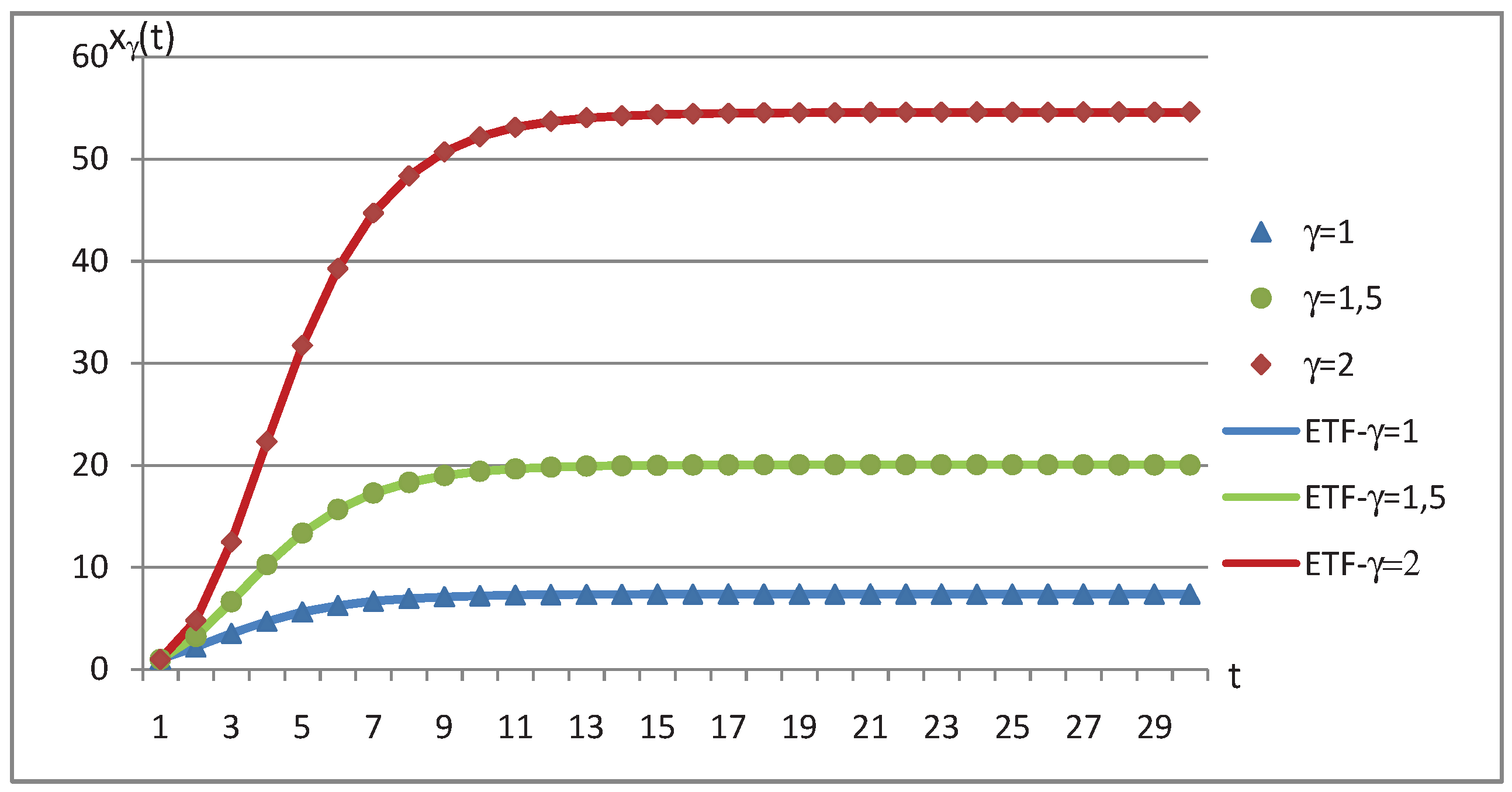
Figure 1. Fit and prediction based on ETF.
Mathematics 08 00588 g001
Figure 2. Fit and prediction based on ETF.
Mathematics 08 00588 g002
Figure 3. Fit and prediction based on ETF.
Mathematics 08 00588 g003
Table 1. Simulated data and estimated trend function.
Time x 1 (t)ETF- x 1 x 1.5 (t)ETF- x 1.5 x 2 (t)ETF- x 2
10.990.990.990.990.990.99
22.18312.18323.23643.23694.79574.7960
33.52723.52716.63806.638512.486112.4876
44.71804.718110.262810.261322.314922.3122
55.62885.628613.364813.362031.734331.7261
66.26516.264515.687815.681839.279639.2767
76.68486.684617.284517.280244.715444.7063
86.95396.953118.331618.327648.360748.3586
97.12207.121118.999818.993350.707550.7176
107.22517.225019.413619.408752.192252.2041
117.28947.288719.670319.664953.118953.1268
127.32857.327719.826219.821953.708853.6943
137.35207.351419.924719.917754.053954.0414
147.36637.365819.977619.976154.259854.2531
157.37427.374620.011720.011554.383654.3818
167.37927.379920.032320.033054.448954.4601
177.38207.383120.049720.046154.490354.5076
187.38417.385120.059820.054054.549254.5364
197.38497.386320.064120.058854.562954.5539
207.38627.387020.064820.061754.562354.5645
217.38757.387420.063320.063554.578354.5710
227.38777.387720.065420.064554.592254.5749
237.38857.387920.066220.065254.599754.5773
247.38827.388020.058720.065654.614854.5787
257.38817.388020.062620.065854.602054.5796
267.38837.388120.063820.066054.591454.5801
277.38907.388120.059920.066154.619654.5804
287.38787.388120.054920.066154.629754.5806
297.38737.388120.050720.066154.611054.5807
Prediction
307.38727.388120.047320.066254.622154.5808
Table 2. Starting values used in the simulation and estimation of the parameters.
σ α β
Starting Values0.000110.5
γ σ ^ α ^ β ^
10.00008520.9999520.500008
1.50.00014981.000430.500377
20.00016061.000030.500052
Table 3. Starting values used in the simulation and estimation of the parameters.
σ α β
Starting values0.000110.5
γ σ ^ α ^ β ^
1.50.00001068011.000060.50003
Table 4. Mean and standard error of the estimators.
hNMean ( σ ^ )SE ( σ ^ )Mean ( α ^ )SE ( α ^ )Mean ( β ^ )SE ( β ^ )
0.051000.0251080.1147361.0001320.0005030.5001440.000439
0.055000.0001120.0000050.9996370.0008390.4997700.000809
0.0510000.0001160.0000051.0001810.0009530.5000900.000915
0.11000.0001060.0000081.0000270.0003500.5000070.000262
0.15000.0001230.0000101.0000200.0006540.5000440.000647
0.110000.0001410.0000160.9990810.0007360.4991560.000672
0.51000.0001430.0000301.0000460.0002530.5000020.000274
0.55000.0003290.0000690.9991710.0006160.4992020.000570
0.510000.0004910.0001410.9985810.0007300.4987790.000584
11000.0002300.0000740.9996100.0003810.4996380.000359
15000.0005840.0002170.9990340.0005970.4990920.000541
110000.0009080.0003180.9975920.0012110.4980450.000923

