On Probability Characteristics for a Class of Queueing Models with Impatient Customers

Abstract

In this paper, a class of queueing models with impatient customers is considered. It deals with the probability characteristics of an individual customer in a non-stationary Markovian queue with impatient customers, the stationary analogue of which was studied previously as a successful approximation of a more general non-Markov model. A new mathematical model of the process is considered that describes the behavior of an individual requirement in the queue of requirements. This can be applied both in the stationary and non-stationary cases. Based on the proposed model, a methodology has been developed for calculating the system characteristics both in the case of the existence of a stationary solution and in the case of the existence of a periodic solution for the corresponding forward Kolmogorov system. Some numerical examples are provided to illustrate the effect of input parameters on the probability characteristics of the system.

1. Introduction

Recently, there has been an increasing interest in studying queueing systems when all the parameters are varying in time; see, for instance, [1]. This is due to the fact that these types of systems are more realistic and the periodic behavior of our daily live in different fields can be treated as well. Some of the examples are call centers, healthcare facilities, arrival and departure clearance for aircraft at airports, security checkpoints, automatic teller machines, multi-car dispatch of police and many others; see for instance [2,3,4] and references therein.

Additionally, queueing models with impatient customers are the subject of research for many papers since they have many applications in telecommunication networks, inventory systems, and impatient telephone switchboard customers; see, for instance, [2,3,4,5,6,7,8,9,10,11,12] and the references in these articles. In the Markovian case, the queue-length process in such systems is a birth–death process, and, in homogeneous situation for a detailed discussion, can be found in [5]. In early studies, the models were studied in such a way that customer impatience was taken into account by a corresponding reduction in arrival rates, see [6,9,10,11,13]. On the other hand, in the last few decades, the property of impatience of customers was treated by the help of increasing ‘death’ rates. Namely, in these models, it is assumed that the customers not only can depart after service (with certain intensities) but also leave the system without service (with corresponding intensities); see, for instance, [3,4].

From a mathematical point of view, both classes of models are described by (inhomogeneous) birth–death processes. Moreover, in the case of a finite number of waiting rooms, the number of states of the process is finite. Therefore, its main properties can be investigated by methods described in details in the paper [14]. If the state space of the queue-length process is countable, one can apply our combined approach which includes bounding on the rate of convergence to the limiting characteristics estimating the error bounds for approximations by truncations, and finally obtaining the perturbation bounds in the case of approximately known intensities. This approach was firstly developed in [15,16,17,18] and described in detail in [19,20].

We would like to draw the attention of the reader to the fact that there are interesting works devoted to a qualitative study of the forward Kolmogorov system for an inhomogeneous continuous-time Markov chains on finite state space; see, for example, [21,22]. Unfortunately, the authors of these studies are apparently not familiar with our earlier papers on this topic, see [16,17,23,24,25].

This article deals with the study of characteristics of an individual customer in a non-stationary queue with impatient customers. The stationary analogue was studied in [3,4] as a successful approximation of a more general non-Markov model which was denoted as an $M\left(n\right)/M\left(n\right)/s/K+M\left(n\right)$ queue.

From a practical point of view, these types of systems can be utilized, for example, in collected water volume dependent releases from dams, speed of traffic on highway depending on the traffic density, and the organization of transmission rates depending on the buffer content in packet-switched telecommunication networks, etc. Note that in the paper all considered processes are assumed to be Markovian ones.

The paper is organized as follows: The model is described and formulated in Section 2. In Section 3 the probability characteristics of the model are presented. In Section 4, an algorithm is proposed to illustrate the steps for computing the probability characteristics. Finally, some numerical examples are discussed in Section 5.

2. Description of the Model

In this paper, we deal with Markovian queueing models with impatient customers assuming that the arrival process is Poisson with intensity function $\lambda \left(t\right).$ The system has s independent servers with the same service rates $\mu \left(t\right)$. When a customer arrives and finds a free server, the service immediately starts; otherwise, it goes to the end of the queue. The service discipline is FIFO (First-In-First-Out queue discipline, also known as First-Come-First-Served). The maximal number of customers in the whole system is denoted by n. Customers staying in the queue are supposed to be impatient; that is, any of the waiting customers can leave the queue with intensity $c\left(t\right).$ The corresponding homogeneous models with impatient customers have been studied in [2,3,4,5,6,7,8,9,10,11,12].

In the papers [6,9,10,11,13], impatience of customers was taken into account by the help of arrival intensities. From a mathematical point of view, the queue-length process of the model was described by a birth–death process. In this paper, we consider a similar model, but, instead of reducing the birth intensities, we increase the death intensities. This approach was applied, for example, in [4,5].

In [5], the authors dealt with the corresponding homogeneous model (i.e., for the situation of constant rates) and proved that the queue-length process $X\left(t\right)$ is a birth–death process with state-dependent intensities. The behavior of an individual customer in the queue is described by a pure death process. As a rule, the authors studied different stationary characteristics of the system.

In this paper, we consider the same model in a non-stationary situation and study a number of important characteristics for the respective queue-length process. We note that the considered queue-length processes are also Markovian ones (certainly, inhomogeneous in time).

Let us start with the notations.

Let $p_{ji}(s,t)=Pr(X\left(t\right)=i|X\left(s\right)=j)$, $0\le i,j\le n$, $0\le s\le t$ and denote by $p_i\left(t\right)$ the corresponding state probabilities for $X\left(t\right)$, $p_i\left(t\right)=Pr(X\left(t\right)=i)$, $0\le i\le n$.

Suppose the following events may happen in $(t,t+h]:$

• exactly one customer enters into the system with probability $\lambda \left(t\right)h+o\left(h\right)$,
• no new customers enter into the system with probability $1-\lambda \left(t\right)h+o\left(h\right)$,
• more than one customer enters into the system with probability $o\left(h\right)$,
• exactly one customer is served with probability $\mu \left(t\right)h+o\left(h\right)$,
• an impatient customer leaves the queue with probability $c\left(t\right)h+o\left(h\right)$,
• and all these events are supposed be independent of each other.

Here, $o\left(h\right)$ is the well-known notation; that is, $o\left(h\right)/h$ tends to zero as $h\to 0$.

Hence, the following transitions are possible for the interval $(t,t+h]$, if $X\left(t\right)=i$:

• $X(t+h)=i+1$ with probability $\lambda \left(t\right)h+o\left(h\right)$ if $0\le i<n$, due to the appearance of a customer in the system,
• $X(t+h)=i-1$ with probability $r_i\left(t\right)h+o\left(h\right),$ where $r_i\left(t\right)=\mu \left(t\right)min(i,s)+c\left(t\right)max(0,i-s),$ if $0<i\le n$, due to the fact that one customer was serviced or left the system,
• $X(t+h)=i$ with probability $1-\lambda \left(t\right)h-r_i\left(t\right)h+o\left(h\right)$ if $0\le i<n$,
• $X(t+h)=n$ with probability $1-r_i\left(t\right)h+o\left(h\right)$ if $i=n$,
• other transitions have probabilities $o\left(h\right)$.

Therefore, $\left\{X\right(t\left)\right|t\ge 0\}$ is a birth–death process with birth and death intensities ${\lambda }_i=\lambda$ and $r_i$ where

$$r_i\left(t\right)=\left\{\begin{array}{cc}i\mu \left(t\right)& i\le s\\ s\mu \left(t\right)+(i-s)c\left(t\right)& n\ge i>s\end{array}\right.$$

(1)

The graph of possible transitions of the process can be drawn as

Denote by $\mathbf{p}\left(t\right)={\left(p_0\left(t\right),p_1\left(t\right),\dots ,p_n\left(t\right)\right)}^T$ the vector of state probabilities at the moment t.

Consider the forward Kolmogorov system of equations in the form

$$\frac{d\left(\mathbf{p}\right(t\left)\right)}{dt}=A\left(t\right)\mathbf{p}\left(t\right).$$

(2)

Hence, our aim is to study this system and compute all the corresponding characteristics of the process $X\left(t\right)$.

For solving this problem, we apply the approach considered for instance in [14]. Namely, using the property ${\sum }_{k=0}^n{p}_k=1$, we put $p_0=1-{\sum }_{k=1}^n{p}_k$. After this, we obtain the reduced forward Kolmogorov system Equation (2) in the form

$$\frac{d\mathbf{z}}{dt}=B\left(t\right)\mathbf{z}+\mathbf{f}\left(t\right),t\ge 0,$$

where $\mathbf{f}\left(t\right)={\left(\lambda \left(t\right),0,\dots ,0\right)}^T$, $\mathbf{z}\left(t\right)={\left(p_1\left(t\right),\dots ,p_n\left(t\right)\right)}^T$, and $b_{ij}\left(t\right)=a_{ij}\left(t\right)-a_{i0}\left(t\right)$. The next step is the study on the rate of convergence for this system which is based on the logarithmic norm of the operator function and the corresponding transformation of the system $\frac{d\left(\mathbf{x}\right(t\left)\right)}{dt}=B\left(t\right)\mathbf{x}\left(t\right)$; the detailed considerations can be seen in our previous papers. Finally, if the intensity functions are constant or periodic in t, we get the bound on the rate of convergence in the form

$$∥{\mathbf{p}}^{*}\left(t\right)-{\mathbf{p}}^{**}\left(t\right)∥\le K{e}^{-\gamma t},$$

for some positive K and $\gamma$, where ${\mathbf{p}}^{*}\left(t\right)$ and ${\mathbf{p}}^{**}\left(t\right)$ are two solutions of system Equation (2) with the corresponding initial conditions ${\mathbf{p}}^{*}\left(0\right)$ and ${\mathbf{p}}^{**}\left(0\right)$. This bound implies ordinary or weak ergodicity of $X\left(t\right)$ in the homogeneous and inhomogeneous situation, respectively. Moreover, in the case of 1-periodic intensities, such bounds give us the possibility of practical computing of the limiting characteristics, see Section 4 and Section 5.

3. The Process Associating with an Individual Customer

Let us start with describing the behavior of an individual customer.

After arrival at moment $t_0$, a customer may

(1)

receives service immediately,

(2)

stand at the end of the queue.

If at the moment of arrival of the tagged customer, there are no waiting rooms in the system and the customer is lost.

Consider the process associated with this customer by $Z\left(t\right)$. Let $Z\left(t\right)=i$ if the customer is in the queue at i-th position, $Z\left(t\right)=0$ if the customer left for service, and $Z\left(t\right)=0^{\prime }$ if the customer left the queue.

Then, for small positive h, the following transitions are possible in the interval $(t,t+h)$ given $Z\left(t\right)=i\ge 1$:

• $Z(t+h)=i-1$ with probability $s\mu \left(t\right)h+(i-1)c\left(t\right)h+o\left(h\right)$ when service or departure from the queue happens for the tagged customer,
• $Z(t+h)=i$ with probability $1-s\mu \left(t\right)h-ic\left(t\right)h+o\left(h\right)$ when there is no changing in the queue,
• $Z(t+h)=0^{\prime }$ with probability $c\left(t\right)h+o\left(h\right)$ if the tagged customer left the queue,
• $o\left(h\right)$ for all other transitions.

Hence, $Z\left(t\right)$ is a pure death process with two absorbing states 0 and $0^{\prime }$, respectively.

The graph of possible transitions of this process has the following form:

Thus, to describe the probabilities of the states of the process $Z\left(t\right)$, we have the following system:

$$\left(\begin{array}{c}\frac{d\left(q_{0^{{}^{\prime }}}\right)}{dt}\\ \frac{d\left(q_0\right)}{dt}\\ \frac{d\left(q_1\right)}{dt}\\ \frac{d\left(q_2\right)}{dt}\\ \dots \\ \frac{d\left(q_{n-s}\right)}{dt}\end{array}\right)=\left(\begin{array}{ccccccc}0& 0& c& c& c& \dots & c\\ 0& 0& s\mu & 0& 0& \dots & 0\\ 0& 0& -c-s\mu & s\mu +c& 0& \dots & 0\\ 0& 0& 0& -2c-s\mu & s\mu +2c& \dots & 0\\ \dots \\ 0& 0& 0& 0& 0& \dots & -s\mu -(n-s)c\end{array}\right)\left(\begin{array}{c}{q}_{0^{{}^{\prime }}}\\ q_0\\ q_1\\ q_2\\ \dots \\ q_{n-s}\end{array}\right)$$

(3)

where all the intensities are the functions of t. Here, the initial conditions are:

$$\begin{array}{c}{q}_{0^{{}^{\prime }}}\left(t_0\right)=0\\ q_0\left(t_0\right)=0\\ q_1\left(t_0\right)=p_s\left(t_0\right)\\ q_2\left(t_0\right)=p_{s+1}\left(t_0\right)\\ \dots \\ q_{n-s}\left(t_0\right)=p_{n-1}\left(t_0\right)\end{array}$$

(4)

Denote by D the event associated with the arrival of the tagged customer at the moment $t_0$.

The probability that an arrival is blocked and lost is $P\left(Loss\right|D)=p_n\left(t_0\right)$.

Let W be the waiting time in the queue for a customer who enters the system at moment $t_0$.

The probability that an arriving customer who enters into the system does not wait at all before its service starts is exactly

$$P(W=0|D)=\frac{1}{1-P\left(Loss\right|D)}\sum _{k=0}^{s-1}{p}_k\left(t_0\right).$$

If D holds, then $q_{0^{{}^{\prime }}}\left(t\right)$ is the probability that the customer leaves from the queue in the interval $[t_0,t)$.

Denote by A the event associated with the departure of the tagged customer from the queue:

$$P\left(A\right|D)=Q_{0^{{}^{\prime }}}=\underset{t\to \infty }{lim}{q}_{0^{{}^{\prime }}}\left(t\right).$$

Then, the conditional distribution function is

$$P(W<t-t_0|AD)=\left\{\begin{array}{cc}\frac{q_{0^{{}^{\prime }}}\left(t\right)}{Q_{0^{{}^{\prime }}}}& t\ge t_0\\ 0& t<t_0.\end{array}\right.$$

The mean conditional waiting time given that the customer eventually abandons is

$$E(t_0,\mathbf{p}\left(t_0\right)|A)=\underset{t\to \infty }{lim}{\int }_{t_0}^t\frac{u-t_0}{Q_{0^{{}^{\prime }}}}\frac{d\left(q_{0^{{}^{\prime }}}\right)}{du}du.$$

Under the assumption D, the probability that a customer who enters the queue completes service in $[t_0,t)$ is $q_0\left(t\right)$.

The probability K that an arrival who enters the queue eventually completes service is

$$P\left(K\right|D)=Q_0=\underset{t\to \infty }{lim}{q}_0\left(t\right).$$

Hence, we obtain the corresponding conditional distribution function:

$$P(W<t-t_0|KD)=\left\{\begin{array}{cc}\frac{q_0\left(t\right)}{Q_0}& t\ge t_0\\ 0& t<t_0\end{array}\right.$$

The mean conditional waiting time given that the customer eventually completes service from queue is

$$E(t_0,\mathbf{p}\left(t_0\right)|K)=\underset{t\to \infty }{lim}{\int }_{t_0}^t\frac{u-t_0}{Q_0}\frac{d\left(q_0\right)}{du}du.$$

The probability that a new arrival who enters the system completes service in $[t_0,t)$ is

$$q\left(t\right)=P(W=0|D)+(1-P(W=0|D)-P\left(Loss\right|D))q_0\left(t\right).$$

Denote by S the event that the service of the tagged customer completes

$$P\left(S\right|D)=Q=P(W=0\left|D\right)+(1-P(W=0\left|D\right)-P\left(Loss\right|D\left)\right)P\left(K\right|D).$$

Then, we have:

$$P(W\le t-t_0|SD)=\left\{\begin{array}{cc}\frac{q\left(t\right)}{Q}& t\ge t_0\\ 0& t<t_0.\end{array}\right.$$

The mean conditional waiting time given that the tagged customer eventually completes service is

$$E(t_0,\mathbf{p}\left(t_0\right)|S)=\underset{t\to \infty }{lim}{\int }_{t_0}^t\frac{u-t_0}{Q}\frac{d\left(q\right)}{du}du.$$

The waiting time distribution of the tagged customer regardless of whether he abandons or is served is

$$P(W\le t-t_0|D)=\left\{\begin{array}{c}P(W=0|D)+(1-P(W=0|D)-\\ P\left(Loss\right|D))(q_{0^{{}^{\prime }}}\left(t\right)+q_0\left(t\right))+P\left(Loss\right|D),& t\ge t_0\\ 0,& t<t_0\end{array}\right..$$

Removing the first and second equation from Equation (3), we can obtain the following estimate for the probability that the tagged customer remains in the queue as follows:

$$\sum _{i=1}^{n-s}{q}_i\left(t\right)\le \left(\sum _{i=1}^{n-s}{q}_i\left(t_0\right)\right)exp\left(-{\int }_{t_0}^{t}c\left(s\right)ds\right).$$

4. Algorithm for Computing the Probability Characteristics

In this section, we summarize the procedure to obtain the probability characteristics with impatient behavior as follows:

1. On the one hand, if the considered Markov chain is homogeneous, one can find the corresponding stationary distribution as the constant solution of system Equation (2). On the other hand, if the process is inhomogeneous and the respective intensities are 1-periodic, then we find the limiting 1-periodic regime by the following way; see details in [14,19] and a brief description in Section 2. First, we obtain the upper bounds for the rate of convergence of the limit mode provided that we start a certain time, say $t^{*}$. The probability characteristics of the process $X\left(t\right)$ do not depend on the initial conditions (up to a given discrepancy). Then, we solve the forward Kolmogorov system with the simplest initial condition $X\left(0\right)=0$ in the interval $[t^{*},t^{*}+1]$. As a result, we obtain all the basic limiting probability characteristics.

2. Consider the ways for obtaining the solutions to system Equation (3). The first approach consists of solving the last equation (with number $n-s$)—then, the equation with number $n-s-1$ and so on. Here, one can use the system of symbolic computation (‘Computer algebra system’). Alternatively, one can apply numerical methods for solving the Cauchy problem for system Equation (3).

3. After finding the solution of Equation (3), we can see that

$$\frac{d\left(q_{0^{{}^{\prime }}}\right)}{dt}=c\left(t\right)\left(q_1\left(t\right)+\dots +q_{n-s}\left(t\right)\right),$$

(5)

$$\frac{d\left(q_0\right)}{dt}=s\mu \left(t\right)q_1\left(t\right),$$

(6)

and therefore we can get formulas without derivatives for instance

$$E(t_0,\mathbf{p}\left(t_0\right)|A)=\underset{t\to \infty }{lim}{\int }_{t_0}^t\frac{u-t_0}{Q_{0^{{}^{\prime }}}}\frac{d\left(q_{0^{{}^{\prime }}}\right)}{du}du=\underset{t\to \infty }{lim}{\int }_{t_0}^t\frac{u-t_0}{Q_{0^{{}^{\prime }}}}c\left(u\right)\sum _{i=1}^{n-s}{q}_i\left(u\right)du,$$

and

$$E(t_0,\mathbf{p}\left(t_0\right)|K)=\underset{t\to \infty }{lim}{\int }_{t_0}^t\frac{u-t_0}{Q_0}\frac{d\left(q_0\right)}{du}du=\underset{t\to \infty }{lim}{\int }_{t_0}^t\frac{u-t_0}{Q_0}s\mu \left(u\right)q_1\left(u\right)du.$$

Regarding initial conditions, the process $X\left(t\right)$ initially affects the average characteristics. However, due to the weak ergodicity of $X\left(t\right)$ at large values of time, the initial conditions cease to have an effect. On the other hand, the initial conditions of the process $Z\left(t\right)$ have a significant effect on the result. These initial conditions $Z\left(t\right)$ can be taken arbitrarily (for example, to analyze the average time of a requirement that falls at a certain place in the queue) or taking into account the behavior of $X\left(t\right)$ (for example, to obtain the average time for a periodic or stationary mode).

5. Numerical Illustrations

In this section, we show several numerical examples to compute the main characteristics for a potential customer in different specific situations.

Note that, unlike other works, here it is shown how to obtain characteristics for requirements arising at a certain place in the queue.

Moreover, our examples show the behavior of the main characteristics of the process associating with an individual customer under different intensities and different initial conditions.

The first situation is devoted to a homogeneous model (i.e., with constant intensities) and a corresponding stationary distribution as an initial one. Our results in this situation coincide with those obtained earlier in the papers [3,4].

The second situation is devoted to the same model and arbitrary initial conditions. Finally, we consider the specific inhomogeneous model with 1-periodic intensities and two different initial conditions for ‘almost limiting 1-periodic’ regime. Note that we use GNU Octave for all numerical examples.

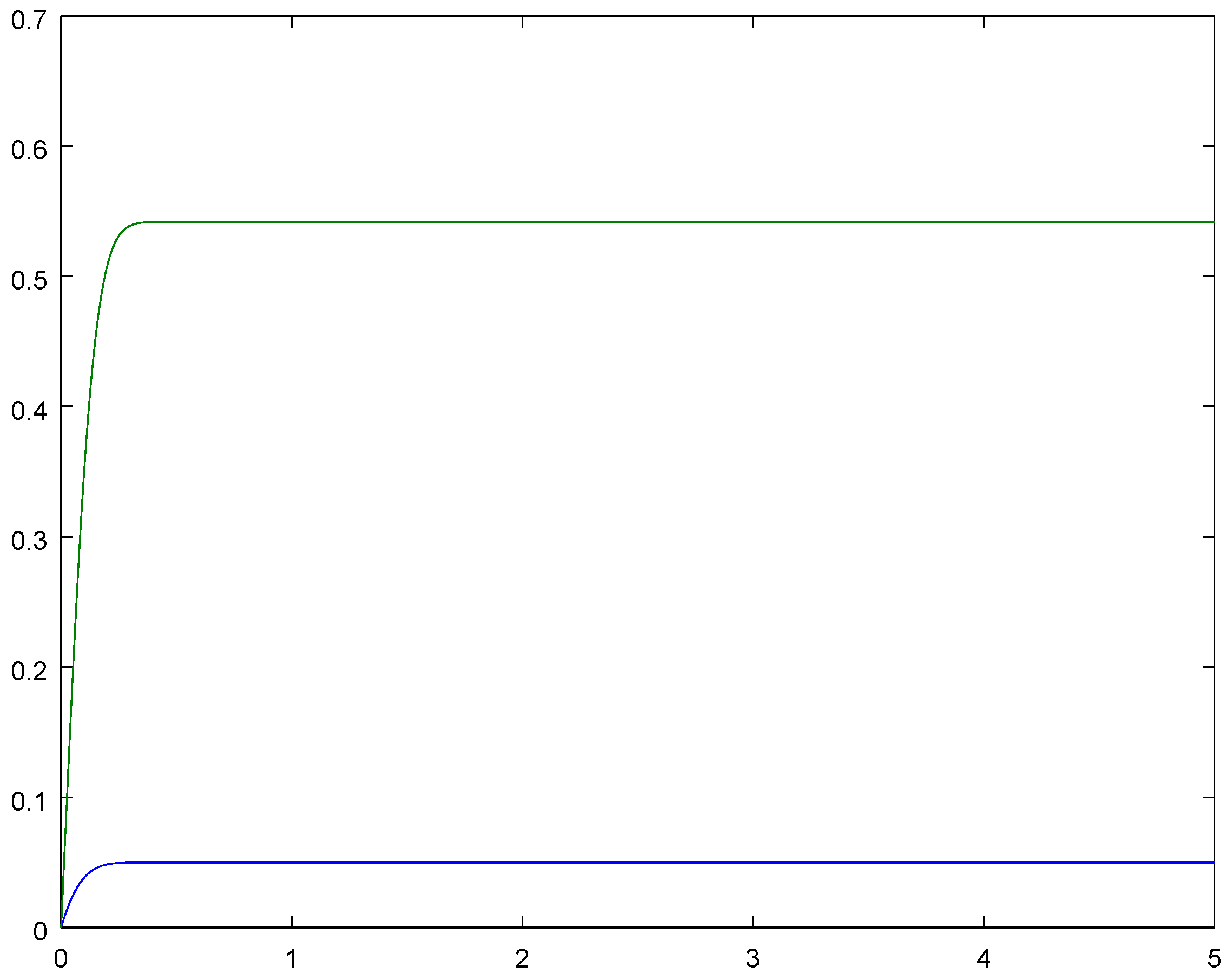
Example 1.

Stationary queueing models with corresponding intensities $\lambda =102$, $\mu =1$, $s=100$, $c=1$. Then, $n=200$ and $r_i=i\mu =i$. Note that, in a stationary (homogeneous in time) situation, the limiting characteristics do not depend on $t_0$. Hence, we will denote such expressions $E(t_0,\mathbf{p}\left(t_0\right)|A)$ by $E\left(W\right|A)$ and so on.

(i)Stationary distribution as initial one. One can find it using forward Kolmogorov system Equation (2) and equation $A{\mathbf{p}}^{*}=0$.

Here, we deal with ${\mathbf{p}}^{*}$ and put $t_0=0$. Hence, $P\left(Loss\right)\approx 0$, $P(W=0)\approx 0.40828$.

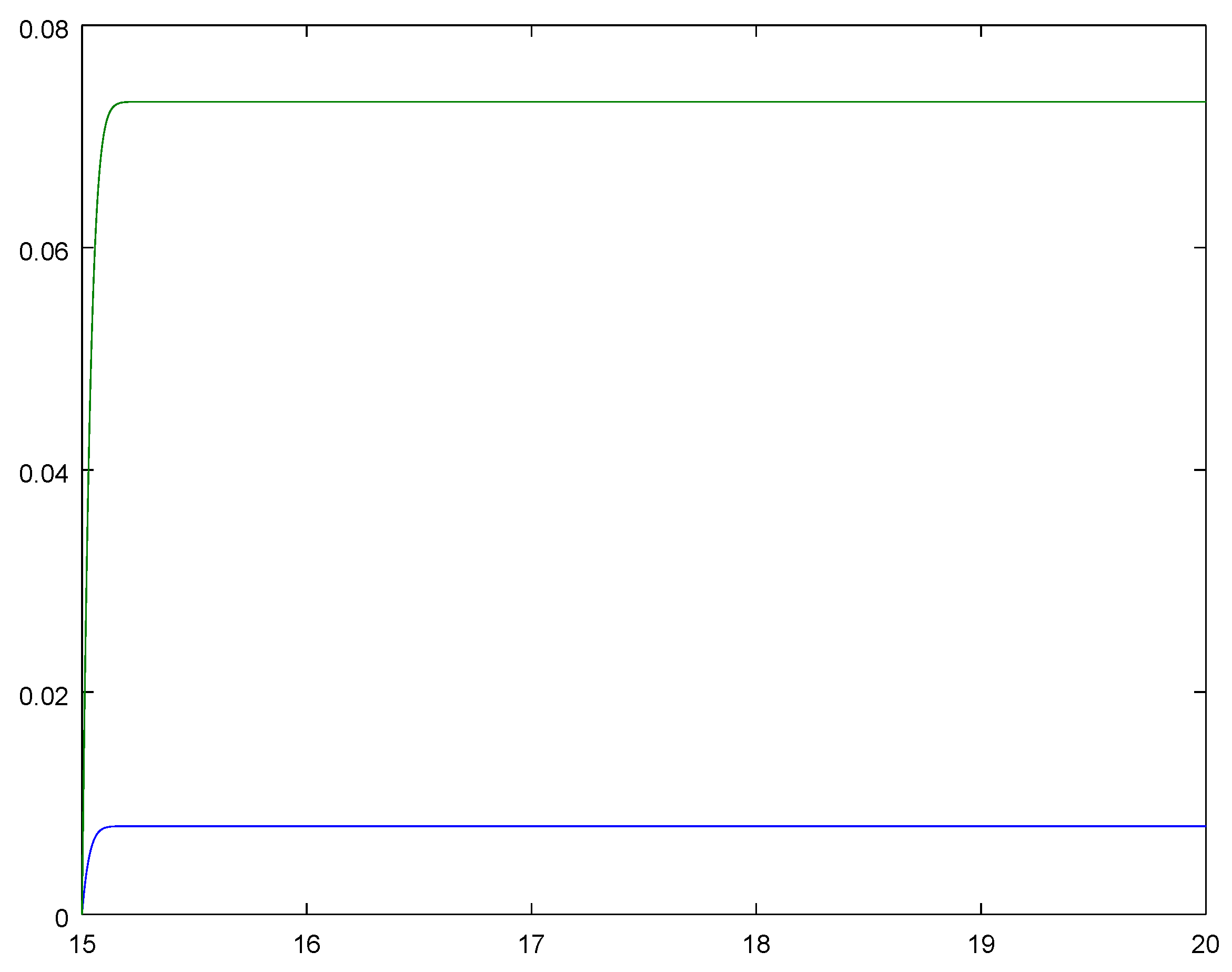
Then, one can compute $q_0\left(t\right)$ and $q_{0^{{}^{\prime }}}\left(t\right)$ from Equation (3). Ergodicity of the process implies closeness of $q_0\left(t\right)$, $q_{0^{{}^{\prime }}}\left(t\right)$ and $Q_0\left(t\right)$, $Q_{0^{{}^{\prime }}}\left(t\right)$, respectively, for sufficiently large t. Therefore, we have $P\left(A\right)=Q_{0^{{}^{\prime }}}\approx q_{0^{{}^{\prime }}}\left(5\right)\approx 0.049918$, $Q_0\approx q_0\left(5\right)\approx 0.541801$; see the corresponding plots in Figure 1.

Now, we can calculate average conditional waiting times, namely

$$E\left(W\right|A)=\underset{t\to \infty }{lim}{\int }_{t_0}^t\frac{u-t_0}{Q_{0^{{}^{\prime }}}}\frac{d\left(q_{0^{{}^{\prime }}}\right)}{du}du\approx {\int }_0^5\frac{u}{Q_{0^{{}^{\prime }}}}\frac{d\left(q_{0^{{}^{\prime }}}\right)}{du}du\approx 0.066611,$$

$$E\left(W\right|K)=\underset{t\to \infty }{lim}{\int }_{t_0}^t\frac{u-t_0}{Q_0}\frac{d\left(q_0\right)}{du}du\approx {\int }_0^5\frac{u}{Q_0}\frac{d\left(q_0\right)}{du}du\approx 0.085997,$$

and

$$E\left(W\right|S)=\underset{t\to \infty }{lim}{\int }_{t_0}^t\frac{u-t_0}{P\left(S\right)}\frac{d\left(q\right)}{du}du\approx {\int }_0^5\frac{u}{P\left(S\right)}\frac{d\left(q\right)}{du}du\approx 0.049042.$$

The corresponding plots (conditional cdf) are shown in Figure 2 and Figure 3.

One can also find the respective conditional probabilities, namely

$$P(W\le 0.1|A)=\frac{q_{0^{{}^{\prime }}}\left(0.1\right)}{Q_{0^{{}^{\prime }}}}\approx 0.76707,$$

$$P(W\le 0.1|K)=\frac{q_0\left(0.1\right)}{Q_0}\approx 0.64691,$$

$$P(W\le 0.1|S)\approx 0.79867,$$

$$P(W\le 0.2|A)=\frac{q_{0^{{}^{\prime }}}\left(0.2\right)}{Q_{0^{{}^{\prime }}}}\approx 0.97016,$$

$$P(W\le 0.2|K)=\frac{q_0\left(0.2\right)}{Q_0}\approx 0.93760,$$

$$P(W\le 0.2|S)\approx 0.96443.$$

(ii)The same model with an arbitrary initial condition of the queue.

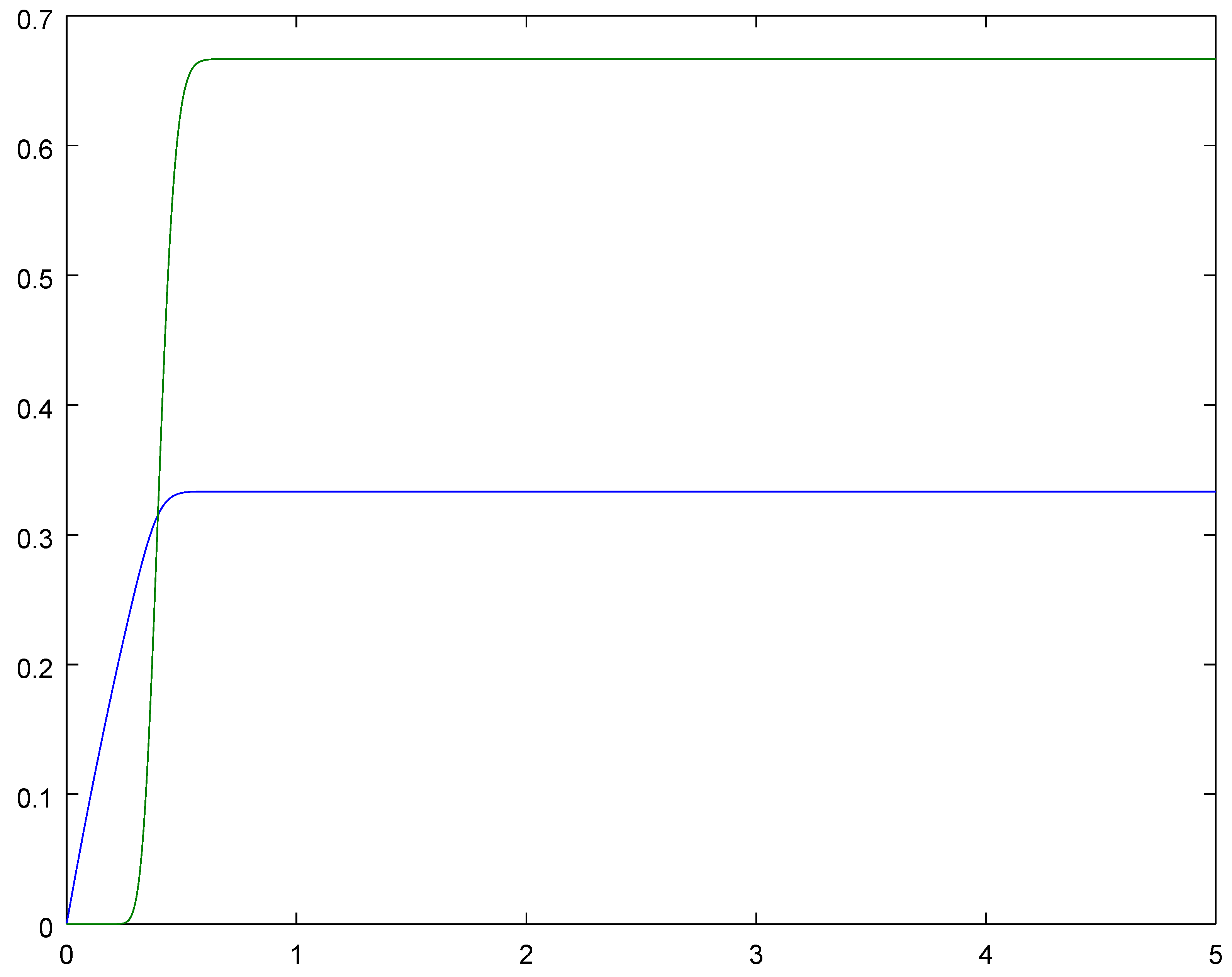
Let there be 149 customers in the system at the initial moment $t_0$ including 100 that are under service and 49 are in the queue, and a new customer arrives into the system (hence, immediately after this moment, there are 150 customers in the system).

Note that, in this way, we get the characteristics for the customers that occupy the 50th place in the queue.

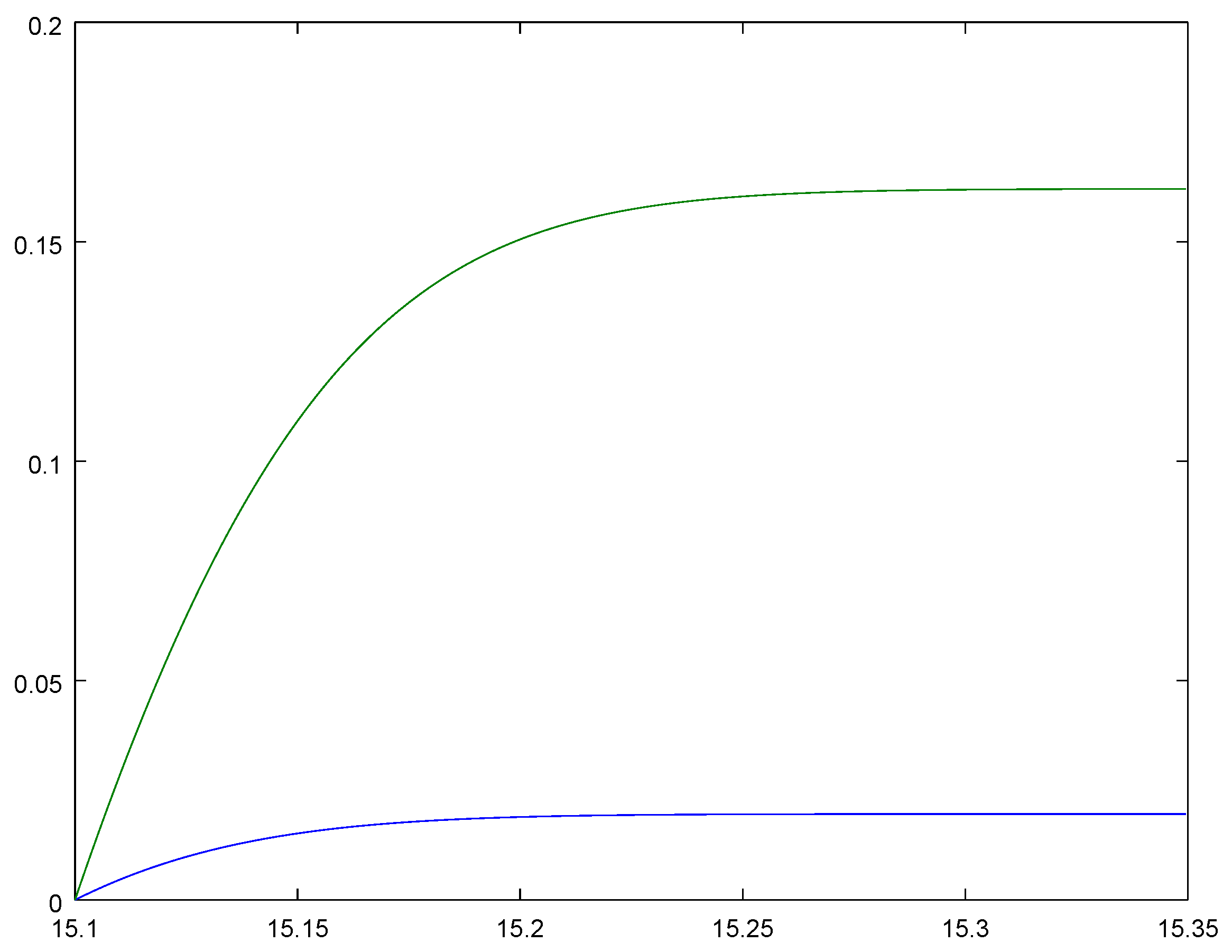
The respective functions $q_0\left(t\right)$ and $q_{0^{{}^{\prime }}}\left(t\right)$ are computed as the corresponding coordinates of the solution of Equation (3) their plots and connection between them are shown in Figure 4.

We have $P\left(A\right)=Q_{0^{{}^{\prime }}}\approx q_{0^{{}^{\prime }}}\left(5\right)\approx 0.33333$ and $Q_0\approx q_0\left(5\right)\approx 0.541801$ and the following corresponding probability characteristics:

$$E\left(W\right|A)=\underset{t\to \infty }{lim}{\int }_{t_0}^t\frac{u-t_0}{Q_{0^{{}^{\prime }}}}\frac{d\left(q_{0^{{}^{\prime }}}\right)}{du}du\approx {\int }_0^5\frac{u}{Q_{0^{{}^{\prime }}}}\frac{d\left(q_{0^{{}^{\prime }}}\right)}{du}du\approx 0.19239,$$

$$E\left(W\right|K)=\underset{t\to \infty }{lim}{\int }_{t_0}^t\frac{u-t_0}{Q_0}\frac{d\left(q_0\right)}{du}du\approx {\int }_0^5\frac{u}{Q_0}\frac{d\left(q_0\right)}{du}du\approx 0.40380,$$

$$E\left(W\right|S)=\underset{t\to \infty }{lim}{\int }_{t_0}^t\frac{u-t_0}{P\left(S\right)}\frac{d\left(q\right)}{du}du\approx {\int }_0^5\frac{u}{P\left(S\right)}\frac{d\left(q\right)}{du}du\approx 0.40380,$$

$$P(W\le 0.1|A)=\frac{q_{0^{{}^{\prime }}}\left(0.1\right)}{Q_{0^{{}^{\prime }}}}\approx 0.28551,$$

$$P(W\le 0.1|K)=\frac{q_0\left(0.1\right)}{Q_0}\approx 0,$$

$$P(W\le 0.1|S)\approx 0,$$

$$P(W\le 0.3|A)=\frac{q_{0^{{}^{\prime }}}\left(0.1\right)}{Q_{0^{{}^{\prime }}}}\approx 0.77673,$$

$$P(W\le 0.3|K)=\frac{q_0\left(0.1\right)}{Q_0}\approx 0.026108,$$

$$P(W\le 0.3|S)\approx 0.026108,$$

$$P(W\le 0.5|A)=\frac{q_{0^{{}^{\prime }}}\left(0.1\right)}{Q_{0^{{}^{\prime }}}}\approx 0.99674,$$

$$P(W\le 0.5|K)=\frac{q_0\left(0.1\right)}{Q_0}\approx 0.94551,$$

$$P(W\le 0.5|S)\approx 0.94551.$$

Example 2.

Non-stationary queueing model with corresponding intensities $\lambda \left(t\right)=102+80sin\left(2\pi t\right)$, $\mu =1$, $s=100$, $c\left(t\right)=2+cos\left(2\pi t\right)$.

1. At first, we compute the limiting periodic solution of the system (2) using the previously developed methods; see [14,19]. For these purposes, it is sufficient to find a solution to this system with the initial condition $\mathbf{p}\left(0\right)={\mathbf{e}}_{\mathbf{0}}$ in the interval $[0,16]$. Hence, in the interval $[15,16]$, we have reasonably accurate approximation of the limiting 1-periodic regime.

2. Let the time of the arrival of a customer $t_0$ vary from 15 to 16. Consider the corresponding queueing characteristics.

2.1. Put now $t_0=15$ and compute the corresponding solution of system (3) in the interval $[15,20]$, where we take the solution of system Equation (2) at the moment $t_0=15$ as an initial condition.

The corresponding characteristics are shown in Figure 5 and Figure 6.

$P\left(A\right)=0.0079420$, $P\left(K\right)=0.073122$.

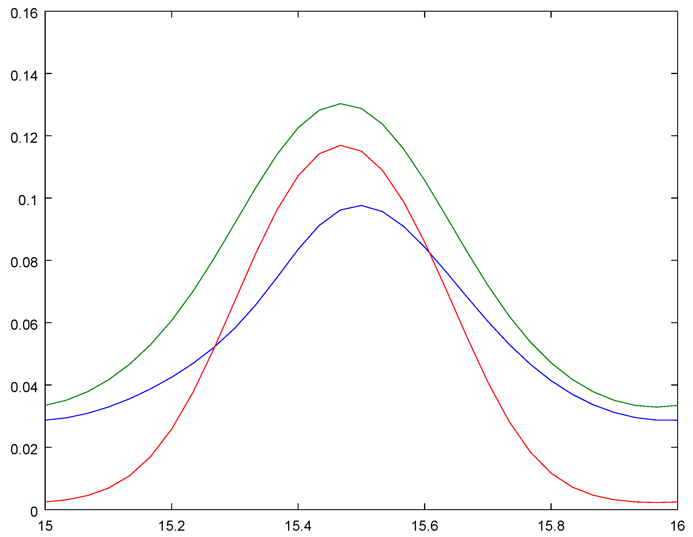
3. Put now $t_0=15.1$ and compute the corresponding solution of system Equation (3) in the interval $[15.1,20.1]$ where we take the solution of system Equation (2) at the moment $t_0=15.1$ as an initial condition.

The corresponding characteristics are shown in Figure 7 and for $t_0=15.1$ we have $P\left(A\right)=0.019595$, $P\left(K\right)=0.16204$.

Similar to the initial condition, we can take the solution of system Equation (2) at any time moment from the interval $[15,16]$. The corresponding mathematical expectations $E(t_0,\mathbf{p}\left(t_0\right)|A)$, $E(t_0,\mathbf{p}\left(t_0\right)|K)$, $E(t_0,\mathbf{p}\left(t_0\right)|S)$ for different $t_0$ are shown in Figure 8.

6. Conclusions

The present paper dealt with non-stationary Markov models of queuing systems with impatient customers. It was shown that the calculation of a number of probabilistic characteristics for such models can be performed by methods used to study the transient properties of birth–death processes. A new mathematical model of the process was considered that describes the behavior of an individual requirement in the requirements queue. This model can be applied both in the stationary and non-stationary cases. Based on the proposed model, a methodology was developed for calculating the probability characteristics of the system both in the case of the existence of a stationary solution and in the case of the existence of a periodic solution for the corresponding forward Kolmogorov system. Several sample examples were presented showing the effectiveness of the proposed methodology. The results obtained are applicable to the study of specific queuing systems, information, and telecommunication systems. In further works, we would like to generalize the results obtained here to different directions: one of the possibilities is weakening the assumptions on the behavior of the processes.