Possibility Measure of Accepting Statistical Hypothesis

Abstract

Taking advantage of the possibility of fuzzy test statistic falling in the rejection region, a statistical hypothesis testing approach for fuzzy data is proposed in this study. In contrast to classical statistical testing, which yields a binary decision to reject or to accept a null hypothesis, the proposed approach is to determine the possibility of accepting a null hypothesis (or alternative hypothesis). When data are crisp, the proposed approach reduces to the classical hypothesis testing approach.

1. Introduction

A statistical hypothesis is a statement of the population distribution. In order to seek evidence for confirming if the hypothesis is true or false, a sample observation needs to be drawn randomly from the population. The major work of this research is, therefore, via selecting a proper statistical method to analyze the collected data and decide whether the null hypothesis under consideration is effective. In classical statistical testing, the sample observations are generally crisp, and all the corresponding testing methods can be well implemented. However, in a practical world, the data are frequently fuzzy due to imprecise measurement and rough description. For example, a survey test for the starting salary of graduated students per year, owing to people unwilling to tell the precise number, the collected sample data are generally fuzzy, and data, such as “roughly $29,000”, “roughly $32,000”, or “less than $40,000”, are obtained. Therefore, the extension of the notion of hypothesis testing to the fuzzy environment would be useful to apply in such a case.

Hypothesis testing methods have been effective for solving problems of fuzzy data. Bellman and Zadeh [1] first introduced hypothesis-testing models for application in the fuzzy environment. Casals et al. [2], Son et al. [3], Römer and Kandel [4], Lubiano et al. [5], and Arefi [6] extended classical statistical hypothesis testing methods to perform hypothesis testing for fuzzy data. Watanabe and Imaizumi [7] also fuzzified the statistical hypothesis and then performed fuzzy testing. Delgado et al. [8] considered a Bayesian testing method for fuzzy data. Arnold [9] considered statistical tests with a continuously distributed test statistic and determined a test to maximize the degree of satisfaction under particular fuzzy requirements. Saade and Schwarzlander [10] discussed hypothesis testing for hybrid data, which is composed of fuzzy data and crisp data. Grzegorzewski [11] presented a corresponding fuzzy testing method by using fuzzy confidence intervals considered by Kruse and Meyer [12]. Filzmoser and Viertl [13] considered testing hypotheses with fuzzy data by the fuzzy p-value. Taheri and Arefi [14] introduced testing fuzzy parametric hypotheses according to a fuzzy test statistic. Wu [15] developed a testing rule as well as a step-by-step procedure by fuzzy critical values and fuzzy p-values when assessing process performance. Parchami et al. [16] presented a method to test hypotheses by comparing a fuzzy p-value and a fuzzy significance level when there were problems with fuzzy hypotheses and crisp data. Alizadeh et al. [17] proposed a hypothesis testing based on a likelihood ratio test for fuzzy hypothesis and fuzzy data. Saeidi et al. [18] considered the problem of testing a hypothesis on the basis of records in a fuzzy environment. Elsherif et al. [19] proposed an algorithm for testing a hypothesis when both hypotheses and data are fuzzy based on a fuzzy test statistic. Habiger [20] developed a framework for the randomized p-value, mid-p-value and abstract randomized p-value, and multiple test function. Icen and Bacanli [21] presented a hypothesis test method for the mean of an inverse Gaussian distribution. In the presented method, confidence intervals by the help of α-cuts are used to obtain a fuzzy test statistic. Yosefi et al. [22] presented an approach for testing fuzzy hypotheses based on a likelihood ratio test statistic. Parchami et al. [23] extended one-way ANOVA to the environment with symmetric triangular and normal fuzzy data. Hesamian and Akbari [24] presented an approach for intuitionistic fuzzy hypotheses by extending the type-I, type-II, power of test, and p-value. Parchami et al. [25] presented a minimax approach to the problem of fuzzy hypotheses while data are crisp. Akbari and Hesamian [26] suggested a degree-based criterion to compare the fuzzy p-value and a specific significance level for making the decision to accept the null hypothesis or not. Kahraman et al. [27] developed interval-valued intuitionistic fuzzy confidence intervals for population mean and differences in means of two populations. Haktanir and Kahraman [28] developed a Z-fuzzy hypothesis testing method. In the developed method, Z-fuzzy numbers are used to capture the vagueness in the sample data, and a Z-fuzzy number is represented by a restriction function that is usually a triangular or trapezoidal fuzzy number. Parchami [29] applied two R packages “FPV” and “Fuzz.p.value” for the practical hypothesis-test problem for when data/hypotheses are fuzzy.

In Theorem 4 of Grzegorzewski [11], the fuzzy test for $H_0:\theta ={\theta }_0$ against the alternative $H_a:\theta \ne {\theta }_0$ is a function $\phi$ with the following α-cuts

$$\phi ({\tilde{X}}_1,\cdots ,{\tilde{X}}_n)=\{\begin{array}{ll}\left\{0\right\}& \mathrm{if}{\theta }_0\in ({\mathsf{\Pi }}_{\alpha }\backslash {(\neg \mathsf{\Pi })}_{\alpha })\\ \left\{1\right\}& \mathrm{if}{\theta }_0\in ({(\neg \mathsf{\Pi })}_{\alpha }\backslash {\mathsf{\Pi }}_{\alpha })\\ \{0,1\}& \mathrm{if}{\theta }_0\in ({\mathsf{\Pi }}_{\alpha }\cap {(\neg \mathsf{\Pi })}_{\alpha })\\ \varphi & \mathrm{if}{\theta }_0\notin ({\mathsf{\Pi }}_{\alpha }\cup {(\neg \mathsf{\Pi })}_{\alpha })\end{array}$$

(1)

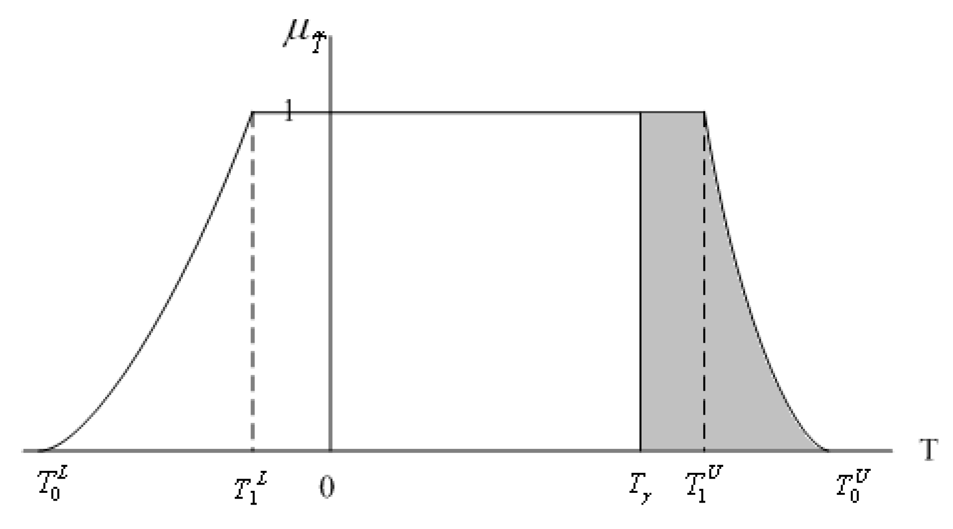
where ${\tilde{X}}_1,{\tilde{X}}_2,\dots ,{\tilde{X}}_n$ are fuzzy random sample, ${\mathsf{\Pi }}_{\alpha }$ is the α-cut of fuzzy confidence interval $\mathsf{\Pi }$ for $\theta$ and ${(\neg \mathsf{\Pi })}_{\alpha }$ is the α-cut of complement of fuzzy confidence interval $\mathsf{\Pi }$. Grzegorzewski [11] claims that the membership function of $\phi$ is ${\mu }_{\phi }(t)={\mu }_{\mathsf{\Pi }}({\theta }_0)I_{\left\{0\right\}}(t)+(1-{\mu }_{\mathsf{\Pi }}({\theta }_0))I_{\left\{1\right\}}(t),$ $t\in \{0,1\}$, where ${\mu }_{\mathsf{\Pi }}({\theta }_0)$ is the membership function value that the parameter value of null hypothesis, ${\theta }_0$, falling in the fuzzy confidence interval $\mathsf{\Pi }$. For example, we get ${\mu }_{\phi }(t)$ = 0.4/0 + 0.6/1 from Figure 1, and the result may be interpreted as “rather reject $H_0:\theta ={\theta }_0$”. Note that, in Figure 1, Grzegorzewski’s approach uses the information on the right-hand side of the fuzzy confidence interval only. This means the testing method of Grzegorzewski [11] is simple but may have some spaces to be improved.

In classical statistical hypothesis testing, the sample data are substituted into a proper test statistic, and the critical value for the test statistic is determined under a given significance level, then the rejection region is determined consequently. When the observed value of the test statistic falls in the rejection region, the null hypothesis should be rejected. Otherwise, the null hypothesis should not be rejected. This is so-called binary decision. Intuitively, when data are fuzzy, the fuzzy testing methods should be developed by fuzzifying the corresponding classical statistical testing methods. Since testing the rejection region is a crisp set, and the observed value of test statistic is fuzzy, we can conduct a reasonable testing approach to determine whether the fuzzy test statistic falls in the rejection region. Moreover, the proposed fuzzy testing method should be able to degenerate to the classical statistical testing method with crisp data. Based on these thoughts, the rest of this paper is organized as follows. Section 2 presents the method to determine whether the fuzzy test statistic falls into the rejection region. Section 3 presents the testing of the normal population to illustrate the real-life application of the proposed method. Section 4 gives examples to compare our proposed approach with the testing methods of Grzegorzewski [11] and Filzmoser and Viertl [13]. Conclusions and suggestions are drawn in Section 5.

2. Fuzzy Test Approach

The fuzzy number can be defined as: given a fuzzy set A of the real line $\Re$, with the membership function ${\mu }_A:\Re \to [0,1]$ satisfies the following conditions:

(a)

A is normal, i.e., there exists an element $x_0$, such that ${\mu }_A(x_0)=1$.

(b)

${\mu }_A(y)\ge \min ({\mu }_A(x),{\mu }_A(z))$, $\forall x\ge y\ge z\in \Re$.

(c)

${\mu }_A$ is upper semicontinuous.

(d)

Support (A) is bounded.

Usually, the α-cut $A_{\alpha }=\{x\in \Re :{\mu }_A(x)\ge \alpha \}$ is used to analyze the fuzzy number. That is, the set $\{A_{\alpha }:\alpha \in [0,1]\}$ is used to describe fuzzy number A.

The probability distribution of the object, $P_{\theta }$, belongs to a distribution family $\wp =\{P_{\theta }:\theta \in \mathsf{\Theta }\}$. Assume that the null hypothesis is $H_0:\theta \in {\mathsf{\Theta }}_0$ and the alternative hypothesis is $H_a:\theta \in {\mathsf{\Theta }}_1$, in which ${\mathsf{\Theta }}_0$ and ${\mathsf{\Theta }}_1$ are the subsets of $\mathsf{\Theta }$, and ${\mathsf{\Theta }}_0\cap {\mathsf{\Theta }}_1=\varphi$. The problem of the classical hypothesis testing problem is that in a set of random sample $X_1{,X}_2,\dots {,X}_n$, the observations can be used to determine to reject $H_0$ (to accept $H_a$) or not to reject $H_0$. The classical testing method is to calculate the probability of a specific test statistic ${T(X}_1{,X}_2,\dots {,X}_n)$ (i.e., the function of observations), to conduct the rejection region C (a crisp set). If the observations of statistic ${T(X}_1{,X}_2,\dots {,X}_n)$ fall into C, then reject the null hypothesis $H_0$; otherwise, do not reject the null hypothesis $H_0$ [30].

When ${\tilde{X}}_1{,\tilde{X}}_2,\dots {,\tilde{X}}_n$ are fuzzy random data, based on the definitions of Kwakernaak [31,32] and Kruse [33], they may be treated as a fuzzy perception of the usual random sample $X_1{,X}_2,\dots {,X}_n$ (see [11]), and $P_{\theta }$ is the population distribution of $X_1{,X}_2,\dots {,X}_n$. Assume that we are interested in testing $H_0:\theta \in {\mathsf{\Theta }}_0$ against $H_a:\theta \in {\mathsf{\Theta }}_1$, and the observed sample data are fuzzy numbers, ${\tilde{X}}_1={\tilde{x}}_1,{\tilde{X}}_2={\tilde{x}}_2,\dots ,{\tilde{X}}_n={\tilde{x}}_n$. By substituting these data into a test statistic ${T(X}_1,X_2,\dots {,X}_n)$, we can obtain a fuzzy number $\tilde{T}={T(\tilde{x}}_1{,\tilde{x}}_2,\dots {,\tilde{x}}_n)$, which are the observations of fuzzy test statistic $T^{*}={T(\tilde{X}}_1{,\tilde{X}}_2,\dots {,\tilde{X}}_n)$. If each membership function of fuzzy number ${\tilde{X}}_i$, ${\mu }_{{\tilde{X}}_i}$ is known, we can obtain the membership function of fuzzy number $\tilde{T}$, ${\mu }_{\tilde{T}}(t)$, by using Zadeh’s extension principle [34]. Fuzzy number $\tilde{T}$ is the observations of fuzzy test statistic $T^{*}=T({\tilde{X}}_1{,\tilde{X}}_2,\dots {,\tilde{X}}_n)$. Therefore, if $\tilde{T}={T(\tilde{x}}_1{,\tilde{x}}_2,\dots {,\tilde{x}}_n)\in C$, then the null hypothesis should be rejected. Otherwise, the null hypothesis should not be rejected. Since $\tilde{T}$ is a fuzzy number, it is not clear whether $\tilde{T}$ falls into the rejection region, C. To solve this problem, Filzmoser and Viertl [13] introduce the concept of a fuzzy p-value. Suppose all α-cuts of $\tilde{T}$ are closed interval ${[t}_1\left(\alpha {),t}_2\right(\alpha \left)\right]$, then each α-cut of $\tilde{T}$ corresponds to a α-cut of fuzzy p-value, which is defined by

$[p_1(\alpha ),p_2(\alpha )]=[P(T\le t_1(\alpha )),P(T\le t_2(\alpha ))]$ for the left-hand sided testing problem,

$[p_1(\alpha ),p_2(\alpha )]=[P(T\le t_1(\alpha ),P(T\le t_2(\alpha )]$ for the right-hand sided testing problem, and

$[p_1(\alpha ),p_2(\alpha )]=\{\begin{array}{c}[2P(T\le t_1(\alpha )),\min [1,2P(T\le t_2(\alpha ))]]\begin{array}{cc}& \mathrm{or}\end{array}\\ [2P(T\ge t_2(\alpha )),\min [1,2P(T\ge t_1(\alpha ))]]\end{array}$ for the two-sided testing problem.

Given the significance level $\gamma$ for all $\alpha \in (0,1]$ and $p_1(\alpha )\le p_2(\alpha )$, the decision of Filzmoser and Viertl [13] is made according to (1) if $p_2(\alpha )<\gamma$, then reject $H_0$ and accept $H_a$; (2) if $p_1(\alpha )>\gamma$, then accept $H_0$ and reject $H_a$; (3) if $\gamma \in [p_1(\alpha ),p_2(\alpha )]$ then both $H_0$ and $H_a$ are neither accepted nor rejected. Note that we cannot make a certain decision in the third case. In this paper, we define the possibility of $\tilde{T}\in C$ and propose another testing approach, so that the total information of a membership function of test statistic can be used, and a fuzzy decision can be made in any case.

Assuming that a fuzzy set A of the real line $\Re$, the membership function of A is ${\mu }_A(y)$, and Zadeh [35] defines that the probability of fuzzy set A is

$$P(A)={\displaystyle {\int }_{\Re }{\mu }_A(y)dP}$$

(2)

where P is the probability measure of Y on real axis $\Re$. Based on Equation (2), we can define:

Definition 1.

The possibility of the value of the fuzzy test statistic,$\tilde{T}$, falling in the rejection region. C is the ratio of probability of$\tilde{T}$to the probability of$\tilde{T}$in C, i.e.,

$$Poss(\tilde{T}\in C)=P(\tilde{T}\in C|T=\tilde{T})\frac{P(T=\tilde{T}and\tilde{T}\in C)}{P(\tilde{T})}\frac{{\displaystyle {\int }_C{\mu }_{\tilde{T}}(t)d{P}_0(t)}}{{\displaystyle {\int }_{\Re }{\mu }_{\tilde{T}}(t)d{P}_0(t)}}$$

(3)

$Poss(\tilde{T}\in C)$= 0, indicates that the possibility of rejecting$H_0$is zero, then we should not reject$H_0$.$Poss(\tilde{T}\in C)$= 1, indicates that the possibility of rejecting$H_0$is 100%, then we should reject$H_0$. If 0 <$Poss(\tilde{T}\in C)=P_0$< 1, this indicates that the possibility of rejecting$H_0$is$P_0$, then we should reject$H_0$with degree of conviction$P_0$. Hence, a fuzzy decision rule is formulated. If a decision maker needs a crisp answer to know whether$H_0$should be rejected or not, the manager can use a random mechanism to transfer the fuzzy decision rule to the binary decision rule. For example, the manager can randomly draw a random number$a$in [0, 1]. If$a\le p_0$, then$H_0$is rejected. If$a>p_0$, then$H_0$is not to be rejected. Consequently, we have a decision rule that is analogous to that of a classical random test.

When data reduce to crisp, the membership function of $\tilde{T}\equiv t_0$ is

$${\mu }_{\tilde{T}}(t)=\{\begin{array}{l}1,t=t_0\\ 0,\mathrm{otherwise}\end{array}.$$

Then, the denominator of Equation (3) is zero, which means that Equation (3) is meaningless. However, since $\tilde{T}\equiv t_0$ is crisp, the possibility of $t_0\in C$ is also crisp. That is, if $t_0\in C$, then $Poss(\tilde{T}\in C)=P(t_0\in C|T=t_0)=1$; if $t_0\notin C$, then $Poss(\tilde{T}\in C)=P(t_0\in C|T=t_0)=0$. This is identical to the classical testing method.

3. Fuzzy Testing of Hypotheses with Fuzzy Data

Suppose the sample data are fuzzy numbers ${\tilde{x}}_1{,\tilde{x}}_2,\dots {,\tilde{x}}_n$. According to Section 2, by substituting these sample data into test statistic $T={T(X}_1{,X}_2,\dots {,X}_n)$, the value $\tilde{T}={T(\tilde{x}}_1{,\tilde{x}}_2,\dots {,\tilde{x}}_n)$ of a fuzzy test statistic $T^{*}$ becomes a fuzzy number. If every membership function of fuzzy number ${\tilde{x}}_i$, ${\mu }_{{\tilde{X}}_i}$ is known, we can obtain the membership function of fuzzy number $\tilde{T}$, ${\mu }_{\tilde{T}}(t)$, by using Zadeh’s extension principle [34].

Represent the α-cuts of ${\tilde{X}}_i$ as

$${(x_i)}_{\alpha }=[{(X_i)}_{\alpha }^L,{(X_i)}_{\alpha }^U]=[{\min }_{\cdot x_i}\{x_i\in X|{\mu }_{{\tilde{X}}_i}(x_i)\ge \alpha \},{\max }_{\cdot x_i}\{x_i\in X|{\mu }_{{\tilde{X}}_i}(x_i)\ge \alpha \}]$$

(4)

where X is the crisp universal set on which ${\tilde{X}}_i$ is defined. It is very difficult to deduce the exact membership function ${\mu }_{\tilde{T}}$ of $\tilde{T}$ because the function relationship may be nonlinear. The approximately membership function ${\mu }_{\tilde{T}}$ can be derived by the approaches of Liu and Kao [36]. Let

$$T_{\alpha }^L=\underset{{(X_i)}_{\alpha }^L\le X_i\le {(X_i)}_{\alpha }^U}{\min .}\left\{T(X_1,X_2,\cdots ,X_n)\right\}$$

(5a)

$$T_{\alpha }^U=\underset{{(X_i)}_{\alpha }^L\le X_i\le {(X_i)}_{\alpha }^U}{\max .}\left\{T(X_1,X_2,\cdots ,X_n)\right\}$$

(5b)

then ${\tilde{T}}_{\alpha }=[T_{\alpha }^L,T_{\alpha }^U]$ is the α-cuts of $\tilde{T}$.

When all fuzzy data reduce to crisp values, Equation (5a,b) become identical and $\tilde{T}$ reduce to $T$ in the classical model. Using Zadeh’s extension principle [34], the membership function ${\mu }_{\tilde{T}}$ may be constructed as

$${\mu }_{\tilde{T}}(t)=\{\begin{array}{ll}0,& t<T_0^L\begin{array}{c}\end{array}or\begin{array}{c}\end{array}t>T_0^U\\ L(t),& T_0^L\le t\le T_1^L\\ 1,& T_1^L\le t\le T_1^U\\ R(t),& T_1^U\le t\le T_0^U\end{array}$$

(6)

where L(t) and R(t) are the left and right shape functions of ${\mu }_{\tilde{T}}$, respectively.

Suppose $H_0:\theta \le {\theta }_0$ against $H_a:\theta >{\theta }_0$ is to be tested and the rejection region is $\{T|T>T_{\gamma }\}$. Figure 2 describes one of the relationships between the membership function ${\mu }_{\tilde{T}}$ and rejection region. The probability of the fuzzy test statistic $\tilde{T}$, based on Equations (2) and (6), is defined as,

$$\Delta ={\displaystyle {\int }_{T_0^L}^{T_1^L}L(t)f(t)dt}+{\displaystyle {\int }_{T_1^L}^{T_1^U}f(t)dt}+{\displaystyle {\int }_{T_1^U}^{T_0^U}R(t)f(t)dt}$$

(7)

where f(t) denotes the probability density function of test statistic T. In Figure 2, based on Equations (3), (6), and (7), the possibility $P_0$ can be defined as,

$$P_0=[{\displaystyle {\int }_{T_{\gamma }}^{T_1^U}f(t)dt}+{\displaystyle {\int }_{T_1^U}^{T_0^U}R(t)f(t)dt}]/\Delta$$

(8)

The right-sided test involves five different types, as shown in Figure 3, where the crisp set $\{T|T>T_{\gamma }\}$ represents the rejection region. Based on Equations (2), (3), (6), and (7), the possibility $P_0$ in Figure 3 are shown in

Table 1. The possibility $P_0$ for the right-sided test.

Case in Figure 3	${\mathit{P}}_0$
(a)	$P_0$ = 0
(b)	$P_0=[{\displaystyle {\int }_{T_{\gamma }}^{T_0^U}}R(t)f(t)dt]/\Delta$
(c)	$P_0=[{\displaystyle {\int }_{T_{\gamma }}^{T_1^U}f(t)dt}+{\displaystyle {\int }_{T_1^U}^{T_0^U}R(t)f(t)dt}]/\Delta$
(d)	$P_0=[{\displaystyle {\int }_{T_{\gamma }}^{T_1^L}}L(t)f(t)dt+{\displaystyle {\int }_{T_1^L}^{T_1^U}}f(t)dt+{\displaystyle {\int }_{T_1^U}^{T_0^U}}R(t)f(t)dt]/\Delta$
(e)	$P_0$ = 1

.

Similarly, the possibility $P_0$ can be calculated for the left-sided test and two-sided test. Figure 4 shows the five different types of the left-sided test, where the rejection region is $\{T|T<T_{1-\gamma }\}$. The definition of possibility $P_0$ is shown in

Table 2. The possibility $P_0$ for left-sided test.

Case in Figure 4	${\mathit{P}}_0$
(a)	$P_0$ = 0
(b)	$P_0=[{\displaystyle {\int }_{T_0^L}^{T_1^L}L(t)f(t)dt}+{\displaystyle {\int }_{T_1^L}^{T_1^U}f(t)dt}+{\displaystyle {\int }_{T_1^U}^{T_{1-\gamma }}R(t)f(t)dt}]/\Delta$
(c)	$P_0=[{\displaystyle {\int }_{T_0^L}^{T_1^L}}L(t)f(t)dt+{\displaystyle {\int }_{T_1^L}^{T_{1-\gamma }}}f(t)dt]/\Delta$
(d)	$P_0=[{\displaystyle {\int }_{T_0^L}^{T_{1-\gamma }}}L(t)f(t)dt]/\Delta$
(e)	$P_0$ = 1

.

The two-sided test involves fifteen different types of membership functions of $\tilde{T}$, as shown in Figure 5, Figure 6 and Figure 7, where the crisp set $\{T|(T<T_{1-\gamma /2})\cup (T>T_{\gamma /2})\}$ is the rejection region. The definition of possibility $P_0$ is shown in

Table 3. The possibility $P_0$ for the two-sided test.

Case in Figure 5, Figure 6 and Figure 7	${\mathit{P}}_0$
(a)	$P_0$ = 1
(b)	$P_0=[{\displaystyle {\int }_{T_0^L}^{T_1^L}L(t)f(t)dt}+{\displaystyle {\int }_{T_1^L}^{T_1^U}f(t)dt}+{\displaystyle {\int }_{T_1^U}^{T_{1-\gamma /2}}R(t)f(t)dt}]/\Delta$
(c)	$P_0=[{\displaystyle {\int }_{T_0^L}^{T_1^L}L(t)f(t)dt}+{\displaystyle {\int }_{T_1^L}^{T_1^U}f(t)dt}+{\displaystyle {\int }_{T_1^U}^{T_{1-\gamma /2}}R(t)f(t)dt}+{\displaystyle {\int }_{T_{\gamma /2}}^{T_0^U}R(t)f(t)dt}]/\Delta$
(d)	$P_0=[{\displaystyle {\int }_{T_0^L}^{T_1^L}}L(t)f(t)dt+{\displaystyle {\int }_{T_1^L}^{T_{1-\gamma /2}}}f(t)dt]/\Delta$
(e)	$P_0=[{\displaystyle {\int }_{T_0^L}^{T_1^L}L(t)f(t)dt}+{\displaystyle {\int }_{T_1^L}^{T_{1-\gamma /2}}f(t)dt}+{\displaystyle {\int }_{T_{\gamma /2}}^{T_0^U}R(t)f(t)dt}]/\Delta$
(f)	$P_0=[{\displaystyle {\int }_{T_0^L}^{T_1^L}L(t)f(t)dt}+{\displaystyle {\int }_{T_1^L}^{T_{1-\gamma /2}}f(t)dt}+{\displaystyle {\int }_{T_{\gamma /2}}^{T_1^U}f(t)dt+{\displaystyle {\int }_{T_1^U}^{T_0^U}R(t)f(t)dt}}]/\Delta$
(g)	$P_0=[{\displaystyle {\int }_{T_0^L}^{T_{1-\gamma /2}}L(t)f(t)dt}]/\Delta$
(h)	$P_0=[{\displaystyle {\int }_{T_0^L}^{T_{1-\gamma /2}}L(t)f(t)dt}+{\displaystyle {\int }_{T_{\gamma /2}}^{T_0^U}R(t)f(t)dt}]/\Delta$
(i)	$P_0$ = 0
(j)	$P_0=[{\displaystyle {\int }_{T_{\gamma /2}}^{T_0^U}R(t)f(t)dt]/}\Delta$
(k)	$P_0=[{\displaystyle {\int }_{T_0^L}^{T_{1-\gamma /2}}L(t)f(t)dt}+{\displaystyle {\int }_{T_{\gamma /2}}^{T_1^U}f(t)dt}+{\displaystyle {\int }_{T_1^U}^{T_0^U}R(t)f(t)dt}]/\Delta$
(l)	$P_0=[{\displaystyle {\int }_{T_{\gamma /2}}^{T_1^U}f(t)dt}+{\displaystyle {\int }_{T_1^U}^{T_0^U}R(t)f(t)dt}]/\Delta$
(m)	$P_0=[{\displaystyle {\int }_{T_0^L}^{T_{1-\gamma /2}}L(t)f(t)dt}+{\displaystyle {\int }_{T_{\gamma /2}}^{T_1^L}L(t)f(t)dt}+{\displaystyle {\int }_{T_1^L}^{T_1^U}f(t)dt}+{\displaystyle {\int }_{T_1^U}^{T_0^U}R(t)f(t)dt}]/\Delta$
(n)	$P_0=[{\displaystyle {\int }_{T_{\gamma /2}}^{T_1^U}}L(t)f(t)dt+{\displaystyle {\int }_{T_1^L}^{T_1^U}}f(t)dt+{\displaystyle {\int }_{T_1^U}^{T_0^U}}R(t)f(t)dt]/\Delta$
(o)	$P_0$ = 1

.

The numerical method is therefore applied to determine the approximate values of $P_0$. As an illustration, we consider some fuzzy testing problems for the normal population with fuzzy data.

3.1. Fuzzy Test of Mean with Known Population Variance

3.1.1. Single Normal Population with Known Population Variance

The mean of a normal population in classical tests generally assumes that the observations are crisp. Suppose that the population variance is known; the test statistic for the null hypothesis about the population mean, $H_0:\mu ={\mu }_0$, is calculated as,

$$Z=\frac{\overline{X}-{\mu }_0}{\sigma /\sqrt{n}}$$

(9)

for a normal population, where $\overline{X}$, n, and $\sigma$ are the sample mean, sample size, and the standard deviation of the population, respectively.

When measured imprecisely, the test statistic using fuzzy data becomes

$$\tilde{Z}\approx \frac{\frac{1}{n}{\displaystyle \sum _{i=1}^n}{\tilde{X}}_i-{\mu }_0}{\sigma /\sqrt{n}}$$

(10)

The exact membership function of a fuzzy test statistic $\tilde{Z}$ can be derived, since the functional relationship between $\tilde{Z}$ and ${\tilde{X}}_i$ is linear. When all the observations ${\tilde{X}}_i$ are trapezoidal fuzzy numbers, the α-cuts of ${\tilde{X}}_i$ can be represented as ${(X_i)}_{\alpha }=[{(X_i)}_{\alpha }^L,{(X_i)}_{\alpha }^U]$. Let

$$Z_{\alpha }^L=\frac{{(\overline{X})}_{\alpha }^L-{\mu }_0}{\sigma /\sqrt{n}}$$

(11a)

$$Z_{\alpha }^U=\frac{{(\overline{X})}_{\alpha }^U-{\mu }_0}{\sigma /\sqrt{n}}$$

(11b)

then ${\tilde{Z}}_{\alpha }=[Z_{\alpha }^L,Z_{\alpha }^U]$ is the α-cuts of $\tilde{Z}$. Equations (11a) and (11b) are a pair of linear functions with bound constraints. The membership function, ${\mu }_{\tilde{Z}}$, is constructed as,

$${\mu }_{\tilde{Z}}(z)=\{\begin{array}{ll}L(z)& ,Z_0^L\le z\le Z_1^L\\ 1& ,Z_1^L\le z\le Z_1^U\\ R(z)& ,Z_1^U\le z\le Z_0^U\\ 0& ,otherwise\end{array}$$

(12)

where $L(z)=(z-Z_0^L)/(Z_1^L-Z_0^L)$ and $R(z)=(Z_0^U-z)/(Z_0^U-Z_1^U)$. $\tilde{Z}$ is also a trapezoidal fuzzy number defined as $\tilde{Z}=[Z_0^L,Z_1^L,Z_1^U,Z_0^U]$, since the function relationship between $\tilde{Z}$ and ${\tilde{X}}_i$ is linear. The trapezoidal membership function ${\mu }_{\tilde{Z}}$ is shown in Figure 8.

Figure 9 shows the right-sided test for $\mu$ under fuzzy data. The probability associated with $\tilde{Z}$, based on Equations (2), (3), and (12), is defined as

$$\Delta ={\displaystyle {\int }_{Z_0^L}^{Z_1^L}}L(z)g(z)dz+{\displaystyle {\int }_{Z_1^L}^{Z_1^U}}g(z)dz+{\displaystyle {\int }_{Z_1^U}^{Z_0^U}}R(z)g(z)dz$$

(13)

where $g(z)$ is the probability density function of a standard normal distribution Z. In Figure 9, the possibility $P_0$ is defined as $P_0=[{\displaystyle {\int }_{Z_{\gamma }}^{Z_1^U}}g(z)dz+{\displaystyle {\int }_{Z_1^U}^{Z_0^U}}R(z)g(z)dz]/\Delta$.

3.1.2. Two Normal Populations with Known Population Variances

This approach can also be applied in a testing hypothesis concerning the difference between two normal population means. Assume the two population variances are known. The classical test statistic of $H_0:{\mu }_X-{\mu }_Y={\mu }_0$ is calculated as,

$$Z=\frac{(\overline{X}-\overline{Y})-{\mu }_0}{\sqrt{\frac{{\sigma }_X^2}{n_X}+\frac{{\sigma }_Y^2}{n_Y}}}$$

(14)

for two independent normal populations. Without loss of generality, assume all data (${\tilde{X}}_i$ and ${\tilde{Y}}_j$) are trapezoidal fuzzy numbers for two independent normal populations with fuzzy data. Equation (14) for calculating the test statistic using fuzzy data becomes,

$$\tilde{Z}\approx \frac{(\frac{1}{n_X}{\displaystyle \sum _{i=1}^{n_X}}{\tilde{X}}_i-\frac{1}{n_Y}{\displaystyle \sum _{j=1}^{n_Y}}{\tilde{Y}}_j)-{\mu }_0}{\sqrt{\frac{{\sigma }_X^2}{n_X}+\frac{{\sigma }_Y^2}{n_Y}}}$$

(15)

Similar to the aforementioned concept, the exact membership function ${\mu }_{\tilde{Z}}$ of $\tilde{Z}$ can be derived. The α-cuts of ${\tilde{X}}_i$ and ${\tilde{Y}}_j$ are represented as,

$$\begin{gathered} {(X_i)}_{\alpha }=[{(X_i)}_{\alpha }^L,{(X_i)}_{\alpha }^U]=[{\min }_{\cdot x_i}\{x_i\in X|{\mu }_{{\tilde{X}}_i}(x_i)\ge \alpha \},{\max }_{\cdot x_i}\{x_i\in X|{\mu }_{{\tilde{X}}_i}(x_i)\ge \alpha \}] \\ {(Y_j)}_{\alpha }=[{(Y_j)}_{\alpha }^L,{(Y_j)}_{\alpha }^U]=[{\min }_{\cdot y_j}\{y_j\in Y|{\mu }_{{\tilde{Y}}_j}(y_j)\ge \alpha \},{\max }_{\cdot y_j}\{y_j\in Y|{\mu }_{{\tilde{Y}}_j}(y_j)\ge \alpha \}] \end{gathered}$$

where ${\mu }_{{\tilde{X}}_i}$ and ${\mu }_{{\tilde{Y}}_j}$ are the membership functions of ${\tilde{X}}_i$ and ${\tilde{Y}}_j$, respectively. Let

$$Z_{\alpha }^L=\frac{[{(\overline{X})}_{\alpha }^L-{(\overline{Y})}_{\alpha }^U]-{\mu }_0}{\sqrt{\frac{{\sigma }_X^2}{n_X}+\frac{{\sigma }_Y^2}{n_Y}}}$$

(16a)

$$Z_{\alpha }^U=\frac{[{(\overline{X})}_{\alpha }^U-{(\overline{Y})}_{\alpha }^L]-{\mu }_0}{\sqrt{\frac{{\sigma }_X^2}{n_X}+\frac{{\sigma }_Y^2}{n_Y}}}$$

(16b)

where ${(\overline{X})}_{\alpha }^L=(1/n_X){\displaystyle {\sum }_{i=1}^{n_X}{(X_i)}_{\alpha }^L}$, ${(\overline{Y})}_{\alpha }^L=(1/n_Y){\displaystyle {\sum }_{j=1}^{n_Y}{(Y_j)}_{\alpha }^L}$, ${(\overline{X})}_{\alpha }^U=(1/n_X){\displaystyle {\sum }_{i=1}^{n_X}{(X_i)}_{\alpha }^U}$ and ${(\overline{Y})}_{\alpha }^U=(1/n_Y){\displaystyle {\sum }_{j=1}^{n_Y}{(Y_j)}_{\alpha }^U}$. When all data are crisp values, Equation (16a,b) become identical and reduce to Equation (14).

3.2. Fuzzy Test of Mean with Unknown Population Variance

3.2.1. Single Normal Population with Unknown Population Variance

The same concept can be applied to cases of an unknown population variance for tests of the mean for a normal population. In the classical statistical test procedure, suppose $\overline{X}$ and S represent the mean and the standard deviation of the sample, respectively. If the null hypothesis $H_0:\mu ={\mu }_0$ is true, then the test statistic

$$T=\frac{\overline{X}-{\mu }_0}{S/\sqrt{n}}$$

(17)

has a t distribution with $n-1$ degrees of freedom when the population is normal.

When the observations are fuzzy, a natural test statistic is obtained by substituting $S^2$ for $(1/n-1){\displaystyle {\sum }_{i=1}^n{({\tilde{X}}_i-(1/n){\displaystyle {\sum }_{i=1}^n{\tilde{X}}_i})}^2}$, in Equation (17), and the fuzzy test statistic becomes,

$$\tilde{T}\approx \sqrt{n}\frac{\frac{1}{n}{\displaystyle \sum _{i=1}^n}{\tilde{X}}_i-{\mu }_0}{\sqrt{\frac{1}{n-1}{\displaystyle \sum _{i=1}^n}{({\tilde{X}}_i-\frac{1}{n}{\displaystyle \sum _{i=1}^n}{\tilde{X}}_i)}^2}}$$

(18)

From Equation (18), the function relationship between $\tilde{T}$ and ${\tilde{X}}_i$ is nonlinear. Deducing the exact membership function ${\mu }_{\tilde{T}}$ is nearly impossible since Equation (18) includes quadratic terms of the fuzzy observations. The lower and upper bounds of α-cuts of fuzzy observations, ${(X_i)}_{\alpha }^L$ and ${(X_i)}_{\alpha }^U$, are calculated. Let

$$T_{\alpha }^L=\underset{{(X_i)}_{\alpha }^L\le X_i\le {(X_i)}_{\alpha }^U}{\min .}\left\{\sqrt{n}\frac{\frac{1}{n}{\displaystyle \sum _{i=1}^n}{X}_i-{\mu }_0}{\sqrt{\frac{1}{n-1}{\displaystyle \sum _{i=1}^n}{(X_i-\frac{1}{n}{\displaystyle \sum _{i=1}^n}{X}_i)}^2}}\right\}$$

(19a)

$$T_{\alpha }^U=\underset{{(X_i)}_{\alpha }^L\le X_i\le {(X_i)}_{\alpha }^U}{\max .}\left\{\sqrt{n}\frac{\frac{1}{n}{\displaystyle \sum _{i=1}^n}{X}_i-{\mu }_0}{\sqrt{\frac{1}{n-1}{\displaystyle \sum _{i=1}^n}{(X_i-\frac{1}{n}{\displaystyle \sum _{i=1}^n}{X}_i)}^2}}\right\}$$

(19b)

then ${\tilde{T}}_{\alpha }=[T_{\alpha }^L,T_{\alpha }^U]$ is the α-cuts of $\tilde{T}$.

${\tilde{T}}_{\alpha }$ is a pair of nonlinear functions with bounded constraints. We can obtain the membership function of fuzzy number $\tilde{T}$, ${\mu }_{\tilde{T}}(t)$, by using Zadeh’s extension principle [34]. When all fuzzy data reduce to crisp values, Equations (19a) and (19b) become identical and reduce to Equation (17) in the classical model.

3.2.2. Two Normal Populations with Unknown but Equal Population Variances

When the two normal population variances are unknown but equal, the test statistic for the null hypothesis about the difference between the two population means, $H_0:{\mu }_X-{\mu }_Y={\mu }_0$, is determined to be

$$T=\frac{(\overline{X}-\overline{Y})-{\mu }_0}{\sqrt{S_P^2(\frac{1}{n_X}+\frac{1}{n_Y})}}$$

(20)

$T$ has a t distribution with $n_X+n_Y-2$ degrees of freedom, where $S_P^2$ represents the pooled sample variance, which is defined as

$$S_P^2=\frac{{\displaystyle \sum _{i=1}^{n_X}}{(X_i-\frac{1}{n_X}{\displaystyle \sum _{i=1}^{n_X}}{X}_i)}^2+{\displaystyle \sum _{j=1}^{n_Y}}{(Y_j-\frac{1}{n_Y}{\displaystyle \sum _{j=1}^{n_Y}}{Y}_j)}^2}{n_X+n_Y-2}$$

When the observations are fuzzy, a natural test statistic substitutes $S_P^2$ for ${\tilde{S}}_P^2$, which is defined as,

$${\tilde{S}}_P^2\approx \frac{{\displaystyle \sum _{i=1}^{n_X}}{({\tilde{X}}_i-\frac{1}{n_X}{\displaystyle \sum _{i=1}^{n_X}}{\tilde{X}}_i)}^2+{\displaystyle \sum _{j=1}^{n_Y}}{({\tilde{Y}}_j-\frac{1}{n_Y}{\displaystyle \sum _{j=1}^{n_Y}}{\tilde{Y}}_j)}^2}{n_X+n_Y-2}$$

Accordingly, Equation (20), for calculating the test statistic when using fuzzy data, becomes,

$$\tilde{T}\approx \frac{(\frac{1}{n_X}{\displaystyle \sum _{i=1}^{n_X}}{\tilde{X}}_i-\frac{1}{n_Y}{\displaystyle \sum _{j=1}^{n_Y}}{\tilde{Y}}_j)-{\mu }_0}{\sqrt{{\tilde{S}}_P^2(\frac{1}{n_X}+\frac{1}{n_Y})}}$$

(21)

From Equation (21), the test statistic is also a fuzzy number. Let

$$T_{\alpha }^L=\underset{\begin{array}{l}{(X_i)}_{\alpha }^L\le X_i\le {(X_i)}_{\alpha }^U\\ {(Y_j)}_{\alpha }^L\le Y_j\le {(Y_j)}_{\alpha }^U\end{array}}{\min .}\left\{\frac{(\frac{1}{n_X}{\displaystyle \sum _{i=1}^{n_X}}{X}_i-\frac{1}{n_Y}{\displaystyle \sum _{j=1}^{n_Y}}{Y}_j)-{\mu }_0}{\sqrt{S_P^2(\frac{1}{n_X}+\frac{1}{n_Y})}}\right\}$$

(22a)

$$T_{\alpha }^U=\underset{\begin{array}{l}{(X_i)}_{\alpha }^L\le X_i\le {(X_i)}_{\alpha }^U\\ {(Y_j)}_{\alpha }^L\le Y_j\le {(Y_j)}_{\alpha }^U\end{array}}{\max .}\left\{\frac{(\frac{1}{n_X}{\displaystyle \sum _{i=1}^{n_X}}{X}_i-\frac{1}{n_Y}{\displaystyle \sum _{j=1}^{n_Y}}{Y}_j)-{\mu }_0}{\sqrt{S_P^2(\frac{1}{n_X}+\frac{1}{n_Y})}}\right\}$$

(22b)

then ${\tilde{T}}_{\alpha }=[T_{\alpha }^L,T_{\alpha }^U]$ is the α-cuts of $\tilde{T}$. When all fuzzy data reduce to crisp values, Equations (22a) and (22b) become identical and reduce to Equation (20) in the classical model. The construction of the membership function ${\mu }_{\tilde{T}}$ and the fuzzy test procedure are the same as those for a single normal population with unknown population variance.

4. Numerical Examples

To illustrate the application of the proposed fuzzy testing method described in Section 3, two examples, in which example 1 is described by Grzegorzewski [11], are presented in this section. Moreover, we will compare the results to that of the testing method of Grzegorzewski [11] and Filzmoser and Viertl [13].

4.1. Example 1

Four random samples $X_1,X_2,X_3,X_4$ are drawn from normal population $N(\theta ,\sigma )$. The perception of these random samples are fuzzy numbers, ${\tilde{x}}_1$ = “roughly between 6 and 8”, ${\tilde{x}}_2$ = “roughly 5”, ${\tilde{x}}_3$ = “roughly 8”, ${\tilde{x}}_4$ = “between 4 and 7”. The membership functions of these data are,

$$\begin{gathered} {\mu }_{{\tilde{X}}_1}(x)=\{\begin{array}{ll}x-5,& 5\le x\le 6\\ 1,& 6\le x\le 8\\ 9-x,& 8\le x\le 9\\ 0,& \mathrm{otherwise}\end{array},{\mu }_{{\tilde{X}}_2}(x)=\{\begin{array}{ll}x-4,& 4\le x\le 5\\ 6-x,& 5\le x\le 6\\ 0,& \mathrm{otherwise}\end{array} \\ {\mu }_{{\tilde{X}}_3}(x)=\{\begin{array}{ll}x-7,& 7\le x\le 8\\ 9-x,& 8\le x\le 9\\ 0,& \mathrm{otherwise}\end{array},{\mu }_{{\tilde{X}}_4}(x)=\{\begin{array}{ll}1,& 4\le x\le 7\\ 0,& \mathrm{otherwise}\end{array} \end{gathered}$$

Assume that standard deviation $\sigma =1$ is known. We are interested in testing $H_0:\theta \le 4.3$ against $H_a:\theta >4.3$, and significance level γ = 0.05. From a classical testing method, we can easily obtain the test statistic as

$$Z=\frac{\overline{X}-{\theta }_0}{\sigma /\sqrt{n}}=\frac{\overline{X}-4.3}{1/\sqrt{4}}=2(\overline{X}-4.3)$$

where $\overline{X}={\displaystyle {\sum }_{i=1}^4{X}_i/4}$ is the sample mean. Therefore, the fuzzy test statistic is

$$\tilde{Z}=\frac{\frac{1}{n}{\displaystyle \sum _{i=1}^n{\tilde{X}}_i}-{\theta }_0}{\sigma /\sqrt{n}}=2(\overline{\tilde{X}}-4.3)$$

where $\overline{\tilde{X}}={\displaystyle {\sum }_{i=1}^4{\tilde{X}}_i/4}$ is the fuzzy sample mean. Based on Zaheh’s extension principle [34], $\overline{\tilde{X}}$ is a trapezoidal fuzzy number [5, 5.75, 7, 7.75], the membership function ${\mu }_{\tilde{Z}}(z)$ of fuzzy number $\tilde{Z}$ is

$${\mu }_{\tilde{Z}}(z)=\{\begin{array}{ll}\frac{1}{1.5}(z-1.4),& 1.4\le z\le 2.9\\ 1,& 2.9\le z\le 5.4\\ \frac{1}{1.5}(6.9-z),& 5.4\le z\le 6.9\\ 0,& \mathrm{otherwise}\end{array}$$

(23)

Since the forth-mentioned rejection region of right-sided testing is $\left\{Z|Z>z_{0.05}=1.645\right\}$, the possibility of $\tilde{Z}\in C$ is

$$Poss(\tilde{Z}\in C)=\frac{{\displaystyle {\int }_{1.645}^{6.9}{\mu }_{\tilde{Z}}(z)\varphi (z)dz}}{{\displaystyle {\int }_{1.4}^{6.9}{\mu }_{\tilde{Z}}}(z)\varphi (z)dz}=\frac{0.0217}{0.0241}=0.901$$

The possibility of rejecting the null hypothesis is 0.901, which is quite high. Grzegorzewski [11] uses the membership function of fuzzy confidence interval $[\overline{\tilde{X}}-z_{0.05}\sigma /\sqrt{n},\infty )$ to determine the testing result. Since the left shape function of the membership function ${\mu }_{\overline{\tilde{X}}}$ is $L(x)=(4/3)(x-4.1775)$. Substituting $\theta =4.3$ into $x$, we can obtain $L(x)=0.1633$. This result is equal to the result of substituting $z=1.645$ into Equation (23), and we can have ${\mu }_{\tilde{Z}}(z)$ = (1.645 − 1.4)/1.5 = 0.1633, which represents the degree of accepting $H_0$. In addition, $1-{\mu }_{\tilde{Z}}(z)=1-0.1633=0.8367$, which represents the degree of rejecting $H_0$. We need to note that, the testing method of Grzegorzewski uses the information of the left shape function $L(x)$ only. However, our proposed method uses all information of $\tilde{Z}$. The fuzzy p-value in Filzmoser and Viertl [13] approximates to a trapezoidal fuzzy number [2.6 × 10⁻¹², 3.33 × 10⁻⁸, 0.00187, 0.0808], we can neither accept nor reject $H_0$ and $H_a$ at significance level γ = 0.05 in this case. If ${\theta }_0$ = 4.93, i.e., we are interested in testing $H_0:\theta \le 4.93$ against $H_a:\theta >4.93$, then the membership function of fuzzy test statistic $\tilde{Z}$ obtained by our proposed method is

$${\mu }_{\tilde{Z}}(z)=\{\begin{array}{ll}\frac{1}{1.5}(z-0.14),& 0.14\le z\le 1.64\\ 1,& 1.64\le z\le 4.14\\ \frac{1}{1.5}(5.64-z),& 4.14\le z\le 5.64\\ 0,& \mathrm{otherwise}\end{array}$$

The possibility of $\tilde{Z}\in C$ is $Poss(\tilde{T}\in C)$ = ${\displaystyle {\int }_{1.645}^{5.64}{\mu }_{\tilde{Z}}(z)\varphi (z)dz/}{\displaystyle {\int }_{0.14}^{5.64}{\mu }_{\tilde{Z}}(z)\varphi (z)dz}$ = 0.24. The result represents that the possibility of rejecting $H_0$ is 24%, and the possibility of accepting $H_0$ is 76%. Note that, with defuzzification, we can reasonably call the trapezoidal fuzzy number $\overline{\tilde{X}}$ = [5, 5.75, 7, 7.75] to be “about 6.375”. The value is 2.89(= (6.375 − 4.93)/0.5) times of the standard deviation as ${\theta }_0$ = 4.93, which is much larger than the critical value 1.645. When using the testing method of Grzegorzewski [11], we have $L(x)=(4/3)(4.93-4.1775)>1$, representing the possibility of accepting $H_0$ is 100%. Therefore, the result obtained by our proposed method is much more reasonable than that obtained by the testing method of Grzegorzewski [11]. The fuzzy p-value in Filzmoser and Viertl [13] approximates to a trapezoidal fuzzy number [8.5 × 10⁻⁹, 1.74 × 10⁻⁵, 0.0505, 0.444], and in this case, we can neither accept nor reject $H_0$ and $H_a$ at significance level γ = 0.05.

4.2. Example 2

Consider the statistical model in Example 1, but to test $H_0:\theta =4$ against $H_a:\theta \ne 4$. Assume that fuzzy sample is ${\tilde{x}}_1$ = “roughly 4.6”, ${\tilde{x}}_2$ = “roughly 5.6”, ${\tilde{x}}_3$ = “roughly 6”, ${\tilde{x}}_4$ = “roughly 3.72”. The membership functions of these data are,

$$\begin{gathered} {\mu }_{{\tilde{X}}_1}(x)=\{\begin{array}{ll}\frac{1}{0.1}(x-4.5),& 4.5\le x\le 4.6\\ \frac{1}{0.2}(4.8-x),& 4.6\le x\le 4.8\\ 0,& \mathrm{otherwise}\end{array},{\mu }_{{\tilde{X}}_2}(x)=\{\begin{array}{ll}\frac{1}{0.1}(x-5.5),& 5.5\le x\le 5.6\\ \frac{1}{0.2}(5.8-x),& 5.6\le x\le 5.8\\ 0,& \mathrm{otherwise}\end{array} \\ {\mu }_{{\tilde{X}}_3}(x)=\{\begin{array}{ll}\frac{1}{0.2}(x-5.8),& 5.8\le x\le 6\\ \frac{1}{0.3}(6.3-x),& 6\le x\le 6.3\\ 0,& \mathrm{otherwise}\end{array},{\mu }_{{\tilde{X}}_4}(x)=\{\begin{array}{ll}\frac{1}{0.12}(x-3.6),& 3.6\le x\le 3.72\\ \frac{1}{0.18}(3.9-x),& 3.72\le x\le 3.9\\ 0,& \mathrm{otherwise}\end{array} \end{gathered}$$

The fuzzy statistic of the two-sided test is

$$\tilde{Z}=\frac{\frac{1}{n}{\displaystyle \sum _{i=1}^n{\tilde{X}}_i-{\theta }_0}}{\sigma /\sqrt{n}}=\frac{\overline{\tilde{X}}-4}{1/\sqrt{4}}=2(\overline{\tilde{X}}-4)$$

Based on Zadeh’s extension principle [34], $\overline{\tilde{X}}$ is a triangular fuzzy number [4.85, 4.98, 5.2]. We can obtain the membership function of fuzzy number, ${\mu }_{\tilde{Z}}(z)$, which is

$${\mu }_{\tilde{Z}}(z)=\{\begin{array}{ll}\frac{1}{0.26}(z-1.7),& 1.7\le z\le 1.96\\ \frac{1}{0.44}(2.4-z),& 1.96\le z\le 2.4\\ 0,& \mathrm{otherwise}\end{array}$$

Under the significance level $\gamma =0.05$, the rejection region is $C=\{Z|\left|Z\right|>z_{0.025}=1.96\}$, and

$$Poss(\tilde{Z}\in C)=\frac{{\displaystyle {\int }_{1.96}^{2.4}{\mu }_{\tilde{Z}}(z)dP}}{{\displaystyle {\int }_{1.7}^{2.4}{\mu }_{\tilde{Z}}(z)dP}}=0.5187$$

Note that the difference between the triangular fuzzy number $\overline{\tilde{X}}$ = [4.85, 4.98, 5.2] and ${\theta }_0$ = 4 is between 1.7 (= (4.85 − 4)/0.5) and 2.4 (= (5.2 − 4)/0.5) times of the standard deviation. When using the testing method of Grzegorzewski [11], we obtain the left shape function of fuzzy confidence interval ($\overline{\tilde{X}}-z_{0.025}(1/\sqrt{4})$) is $L(x)=(1/0.13)(x-3.87),3.87<x\le 4$. When ${\theta }_0$ = 4, $L(x)=1$, representing the possibility of accepting $H_0$ is 100%. Apparently, the result obtained by our proposed method is much more reasonable than that obtained by the testing method of Grzegorzewski [11]. The fuzzy p-value in Filzmoser and Viertl [13] approximates to a triangular fuzzy number [0.0164, 0.05, 0.0719], we can neither accept nor reject $H_0$ and $H_a$ at significance level γ = 0.05 in this case. If we consider the significance level $\gamma =0.08$, the rejection region is $C=\{Z|\left|Z\right|>z_{0.04}=1.75\}$, and

$$Poss(\tilde{Z}\in C)=\frac{{\displaystyle {\int }_{1.75}^{2.4}{\mu }_{\tilde{Z}}(z)dP}}{{\displaystyle {\int }_{1.7}^{2.4}{\mu }_{\tilde{Z}}(z)dP}}=0.9772$$

Hence, $H_0$ is rejected with very high possibility at the level γ = 0.08. However, when using the testing method of Grzegorzewski [11], the left shape function of fuzzy confidence interval ($\overline{\tilde{X}}-z_{0.04}(1/\sqrt{4})$) is $L(x)=(1/0.13)(x-3.975),3.975<x\le 4.105$. When ${\theta }_0$ = 4, $L(x)=0.1923$, representing that the possibility of accepting $H_0$ is 19.23%. Using fuzzy p-value in Filzmoser and Viertl [13], we conclude that $H_0$ is rejected at the level γ = 0.08, which is close to the result of ours. If significance level $\gamma =0.1$, then Grzegorzewski [11], Filzmoser and Viertl [13], and our method have the same conclusion that the null hypothesis $H_0$ is rejected.

5. Conclusions

In this paper, we propose a fuzzy test approach for the hypothesis testing of fuzzy data, which is an extension of a classical method of statistical hypothesis testing of crisp data. The proposed approach first utilizes the probability of fuzzy sets to conduct the possibility definition that fuzzy test statistics fall in the rejection region, and then results in a fuzzy decision rule to determine whether the null hypothesis is to be rejected or not. Although the proposed approach is similar to the fuzzy testing method of Grzegorzewski [11], which is conducted by using confidence intervals, our method is more direct and clear since we use fuzzy test statistics directly. In addition, the latter only uses the single point information on the membership function of the fuzzy confidence interval to make a fuzzy decision rule for the possibility of accepting the null hypothesis. Apparently, when we make decisions, the information used in our proposed approach is much more reasonable and effective than that of Grzegorzewski [11]. Moreover, though our proposed approach is similar to the fuzzy testing method of Filzmoser and Viertl [13], in the latter approach, we can neither accept nor reject $H_0$ and $H_a$ at significance level γ if the value of membership function of the fuzzy p-value at γ is not zero, while our method can make a clear decision in any case. Therefore, our method is more flexible and useful than Filzmoser and Viertl [13]. Although we only present the testing of a single normal population as the illustrative examples, our proposed approach can be applied to all the classical testing methods for fuzzy data. Therefore, the proposed approach is simple and useful.

References

1. Bellman, R.E.; Zadeh, L.A. Decision-making in a fuzzy environment. Manag. Sci. 1970, 17, 141–164. [Google Scholar] [CrossRef]
2. Casals, R.; Gil, M.A.; Gil, P. On the use of Zadeh’s probabilistic definition for testing statistical hypotheses from fuzzy information. Fuzzy Sets Syst. 1986, 20, 175–190. [Google Scholar] [CrossRef]
3. Son, J.C.; Song, I.; Kim, H.Y. A fuzzy decision problem based on the generalized Neyman-Pearson criterion. Fuzzy Sets Syst. 1992, 47, 65–75. [Google Scholar]
4. Römer, C.; Kandel, A. Statistical tests for fuzzy data. Fuzzy Sets Syst. 1995, 72, 1–26. [Google Scholar] [CrossRef]
5. Lubiano, M.A.; Salas, A.; Gil, M.A. A hypothesis testing-based discussion on the sensitivity of means of fuzzy data with respect to data shape. Fuzzy Sets Syst. 2017, 328, 54–69. [Google Scholar] [CrossRef]
6. Arefi, M. Testing statistical hypotheses under fuzzy data and based on a new signed distance. Iran. J. Fuzzy Syst. 2018, 15, 153–176. [Google Scholar]
7. Watanabe, N.; Imaizumi, T. A fuzzy statistical test of fuzzy hypotheses. Fuzzy Sets Syst. 1993, 53, 167–178. [Google Scholar] [CrossRef]
8. Delgado, M.; Verdegay, J.L.; Vila, M.A. Testing fuzzy hypotheses. A Bayesian approach. In Approximate Reasoning in Expert Systems; Gupta, M.M., Kandel, A., Bandler, W., Kiszka, J.B., Eds.; Elsevier: Amsterdam, The Netherlands, 1985; pp. 307–316. [Google Scholar]
9. Arnold, B.F. Statistical tests optimally meeting certain fuzzy requirements on the power function and on the sample size. Fuzzy Sets Syst. 1995, 75, 365–372. [Google Scholar] [CrossRef]
10. Saade, J.J.; Schwarzlander, H. Fuzzy hypothesis testing with hybrid data. Fuzzy Sets Syst. 1990, 35, 197–212. [Google Scholar] [CrossRef]
11. Grzegorzewski, P. Testing statistical hypotheses with vague data. Fuzzy Sets Syst. 2000, 112, 501–510. [Google Scholar] [CrossRef]
12. Kruse, R.; Meyer, K.D. Confidence intervals for the parameters of a linguistic random variable. In Combining Fuzzy Imprecision with Probabilistic Uncertainty in Decision Making; Kacprzyk, J., Fedrizzi, M., Eds.; Springer: Berlin/Heidelberg, Germany, 1988; pp. 113–123. [Google Scholar]
13. Filzmoser, P.; Viertl, R. Testing hypotheses with fuzzy data: The fuzzy p-value. Metrika 2004, 59, 21–29. [Google Scholar] [CrossRef]
14. Taheri, S.M.; Arefi, M. Testing fuzzy hypotheses based on fuzzy test statistic. Soft Comput. 2009, 13, 617–625. [Google Scholar] [CrossRef]
15. Wu, C.W. Decision-making in testing process performance with fuzzy data. Eur. J. Oper. Res. 2009, 193, 499–509. [Google Scholar] [CrossRef]
16. Parchami, A.; Taheri, S.M.; Mashinchi, M. Fuzzy p-value in testing fuzzy hypotheses with crisp data. Stat. Pap. 2010, 51, 209–226. [Google Scholar] [CrossRef]
17. Alizadeh, H.M.; Khamseh, A.R.A.; Ghomi, S.M.T.F. Fuzzy hypothesis testing with vague data using likelihood ratio test. Soft Comput. 2013, 17, 1629–1641. [Google Scholar] [CrossRef]
18. Saeidi, A.R.; Akbari, M.G.; Doostparast, M. Hypotheses testing with the two-parameter Pareto distribution on the basis of records in fuzzy environment. Hybernetika 2014, 50, 744–757. [Google Scholar]
19. Elsherif, A.K.; Tang, C.M.; Zhang, L. Fuzzy hypotheses testing using fuzzy data and confidence interval in radar decision criteria. Evol. Syst. 2015, 6, 67–74. [Google Scholar] [CrossRef]
20. Habiger, J.D. Multiple test functions and adjusted p-values for test statistics with discrete distributions. J. Stat. Plan. Inference 2015, 167, 1–13. [Google Scholar] [CrossRef]
21. Icen, D.; Bacanli, S. Hypothesis testing for the mean of inverse Gaussian distribution using alpha-cuts. Soft Comput. 2015, 19, 113–119. [Google Scholar] [CrossRef]
22. Yosefi, S.; Arefi, M.; Akbari, M.G. A new approach for testing fuzzy hypotheses based on likelihood ratio statistic. Stat. Pap. 2016, 57, 665–688. [Google Scholar] [CrossRef]
23. Parchami, A.; Nourbakhsh, M.; Mashinchi, M. Analysis of variance in uncertain environments. Complex Intell. Syst. 2017, 3, 189–196. [Google Scholar] [CrossRef] [Green Version]
24. Hesamian, G.; Akbari, M.G. Statistical test based on intuitionistic fuzzy hypotheses. Commun. Stat. Theory Methods 2017, 46, 9324–9334. [Google Scholar] [CrossRef]
25. Parchami, A.; Taheri, S.M.; Viertl, R.; Mashinchi, M. Minimax test for fuzzy hypotheses. Stat. Pap. 2018, 59, 1623–1648. [Google Scholar] [CrossRef]
26. Akbari, M.G.; Hesamian, G. Testing statistical hypotheses for intuitionistic fuzzy data. Soft Comput. 2019, 23, 10385–10392. [Google Scholar] [CrossRef]
27. Kahraman, C.; Oztaysi, B.; Onar, S.C. Interval-valued intuitionistic fuzzy confidence intervals. Int. J. Intell. Syst. 2019, 28, 307–319. [Google Scholar] [CrossRef]
28. Haktanir, E.; Kahraman, C. Z-fuzzy hypothesis testing in statistical decision making. J. Intell. Fuzzy Syst. 2019, 37, 6545–6555. [Google Scholar] [CrossRef]
29. Parchami, A. Fuzzy decision making in testing hypotheses: An introduction to the packages “FPV” and “Fuzzy. p value” with practical examples. Iran. J. Fuzzy Syst. 2020, 17, 67–77. [Google Scholar]
30. Lehmann, E.L. Testing Statistical Hypotheses, 2nd ed.; Wiley: New York, NY, USA, 1986. [Google Scholar]
31. Kwakernaak, H. Fuzzy random variables, part I: Definitions and theorems. Inf. Sci. 1978, 15, 1–15. [Google Scholar] [CrossRef] [Green Version]
32. Kwakernaak, H. Fuzzy random variables, part II: Algorithms and examples for the discrete case. Inf. Sci. 1978, 17, 253–278. [Google Scholar] [CrossRef] [Green Version]
33. Kruse, R. The strong law of large numbers for fuzzy random variables. Inf. Sci. 1982, 28, 233–241. [Google Scholar] [CrossRef]
34. Zimmermann, H.J. Fuzzy Set Theory and Its Applications, 3rd ed.; Kluwer-Nijhoff: Boston, MA, USA, 1996. [Google Scholar]
35. Zadeh, L.A. Probability measures of fuzzy events. J. Math. Anal. Appl. 1968, 23, 421–427. [Google Scholar] [CrossRef] [Green Version]
36. Liu, S.T.; Kao, C. Solving fuzzy transportation problems based on extension principle. Eur. J. Oper. Res. 2004, 153, 661–674. [Google Scholar] [CrossRef]
Figure 1. Testing function φ of Grzegorzewski [11].
Mathematics 08 00551 g001
Figure 2. The membership function μ T ˜ and rejection region {   T   |   T > T γ } .
Mathematics 08 00551 g002
Figure 3. Five different types of membership functions of T ˜ for the right-sided test.
Mathematics 08 00551 g003
Figure 4. Five different types of membership functions of T ˜ for the left-sided test.
Mathematics 08 00551 g004
Figure 5. Left-tended five different types of membership functions of T ˜ for the two-sided test.
Mathematics 08 00551 g005
Figure 6. Centralized five different types of membership functions of T ˜ for the two-sided test.
Mathematics 08 00551 g006
Figure 7. Right-tended five different types of membership functions of T ˜ for the two-sided test.
Mathematics 08 00551 g007
Figure 8. Membership function of Z ˜ .
Mathematics 08 00551 g008
Figure 9. The right-sided test for μ under fuzzy data.
Mathematics 08 00551 g009