A Mathematical Pre-Disaster Model with Uncertainty and Multiple Criteria for Facility Location and Network Fortification

Abstract

Disasters have catastrophic effects on the affected population, especially in developing and underdeveloped countries. Humanitarian Logistics models can help decision-makers to efficiently and effectively warehouse and distribute emergency goods to the affected population, to reduce casualties and suffering. However, poor planning and structural damage to the transportation infrastructure could hamper these efforts and, eventually, make it impossible to reach all the affected demand centers. In this paper, a pre-disaster Humanitarian Logistics model is presented that jointly optimizes the prepositioning of aid distribution centers and the strengthening of road sections to ensure that as much affected population as possible can efficiently get help. The model is stochastic in nature and considers that the demand in the centers affected by the disaster and the state of the transportation network are random. Uncertainty is represented through scenarios representing possible disasters. The methodology is applied to a real-world case study based on the 2018 storm system that hit the Nampula Province in Mozambique.

1. Introduction

After a disaster strikes a territory it is imperative to deliver relief items to the affected population to reduce human casualties and suffering. This is especially true in underdeveloped and developing countries that suffer from a lack of resources and reliable infrastructures. Additionally, poor planning and structural damage to the transportation network could hinder the relief effort or, in some cases, completely frustrate them. Damaged roads, resulting from the effect of the disaster, could completely disconnect affected populations from the rest of the transportation network, thus, making impossible to undertake any relief operation. This was the case in Haiti, after the 2010 earthquake, where, despite the large volume of emergency goods available, the victims could not receive support for a long time due to the damage suffered by the road network [1,2,3,4]. The 2011 Japan earthquake and tsunami interdicted about three-fourths of the highways in the region, hampering the emergency response operations [5]. More recently in Puerto Rico, after Hurricane Maria hit the island in 2017, shortages in vehicle drivers and disruptions to the road network made it impossible to deliver emergency supplies, including food, water, and medicine, resulting in at least 10,000 containers idly sitting at the port [6]. Locating emergency inventories and fortifying vulnerable elements of the road infrastructure prior to an emergency helps to mitigate the impact of a disaster, facilitates the relief operations, and increases the effectiveness of the disaster response.

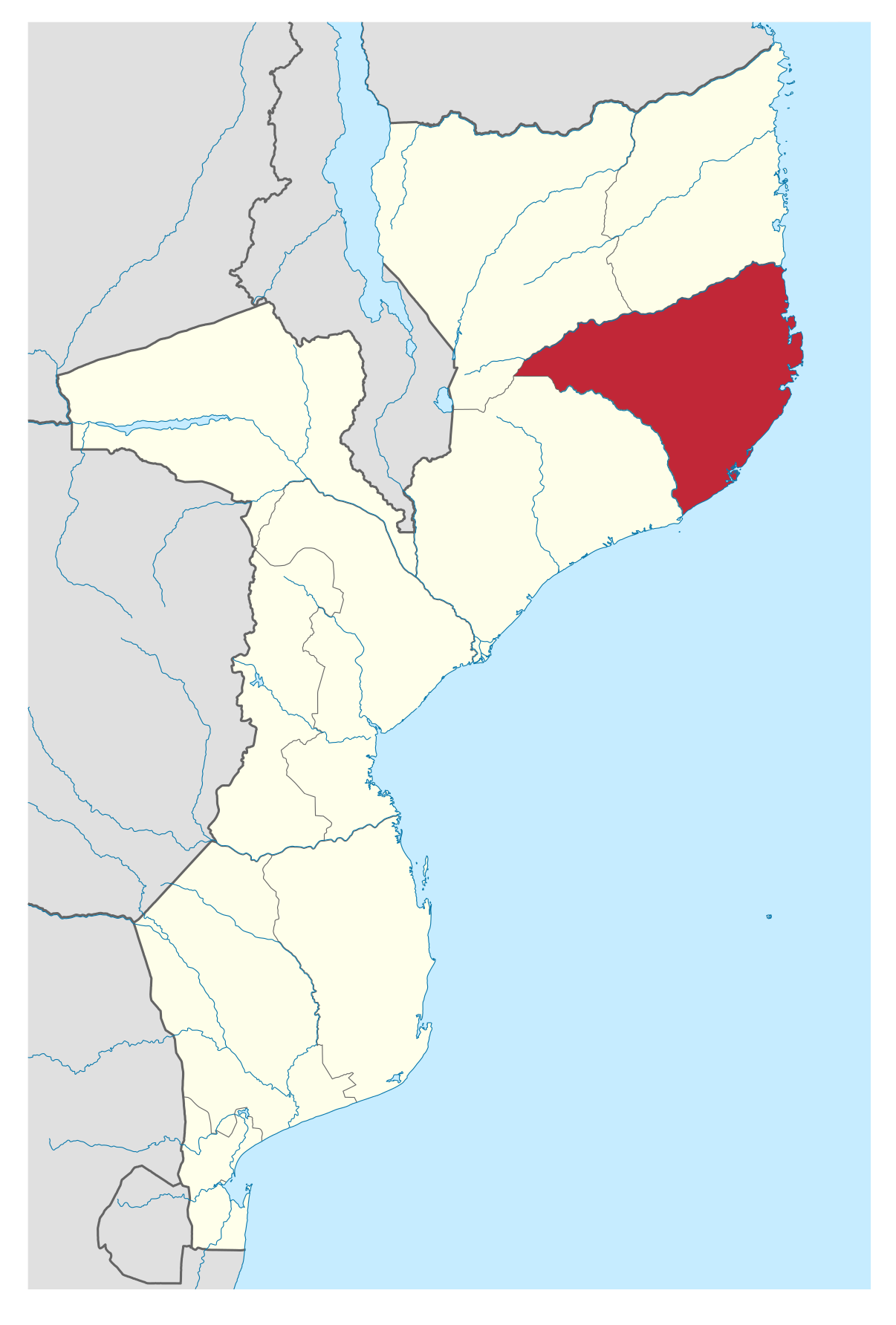
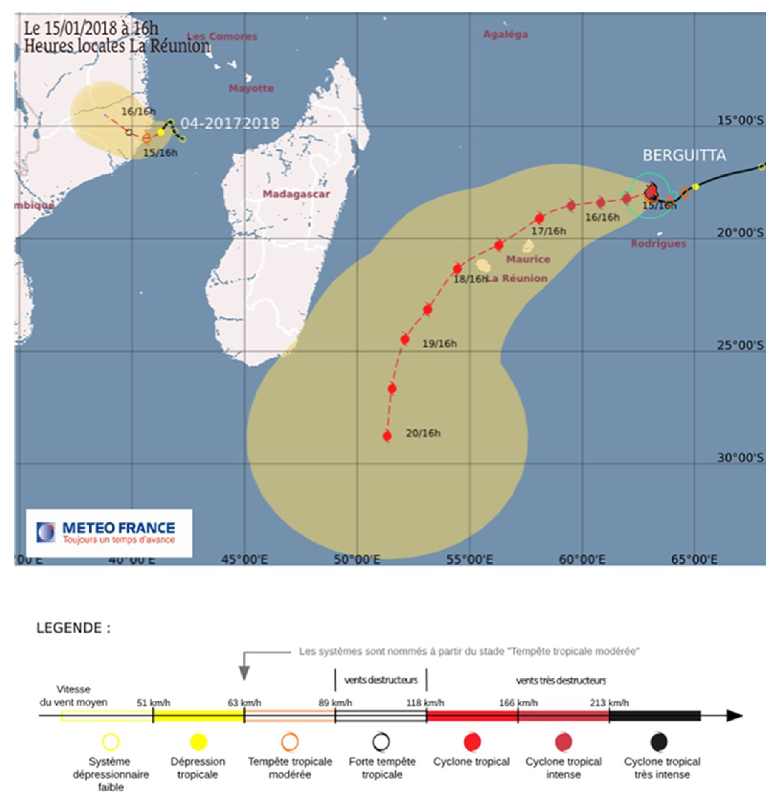
In this paper, a pre-disaster model that tackles these issues is proposed. The model jointly optimizes the fortification of elements of the distribution network, the location of emergency inventories, and the definition of their capacity. The goal is to support the distribution operations of relief goods in the best possible way. Due to the uncertainty that characterizes disasters, the model is stochastic in nature. Multiple objectives are considered. However, the objective of minimizing the expected unsatisfied demand has the highest priority, as not providing relief to populations affected by a disaster might result in human casualties. This objective has multiple optima, therefore, the optimal solutions are further evaluated according to two time measures: the expected maximum arrival time at a demand node and the expected total service time. The computational experiments show little trade-off between these time criteria. For this reason, the solutions are evaluated using a pay-off matrix, rather than by applying specific multicriteria methods. More generally, the methodology has been designed to be applicable in situations with limited data on the availability of resources and the status of the road infrastructure, which is especially relevant to underdeveloped and developing countries. In fact, the model has been tailored to a real case study on the 2018 tropical depression that hit the Nampula Province (Mozambique) and considers only the data that could be obtained from official sources. For this reason, and given its focus on pre-disaster operations, the model relies on a number of simplifying assumptions concerning the distribution operations. For instance, these are represented by an underlying flow model. As a consequence, most details of a real supply chain are disregarded, such as, multiple commodities, multiple transportation modes, vehicles availability and capacity, and distribution queues. However, this is consistent with the application context and the scope of the model.

1.1. Literature Review

According to Anysia and Kopczak [7], Humanitarian Logistics is “the process of planning, implementing and controlling the efficient, cost-effective flow and storage of goods and materials, as well as related information, from the point of origin to the point of consumption for the purpose of alleviating the suffering of vulnerable people.” The seminal work by Aghani and Oh [8] presents a large-scale multi-commodity multi-modal network flow model with time windows in the context of disaster relief operations, which the authors solve using heuristics. In recent years, due to the relevance of the subject, the investigation in Humanitarian Logistics models has experienced a golden age and a wealth of research contributions have been published. Due to the large number of works in the field, the review presented in this paper focuses on relief distribution models that combine location operations with structural operations on the transportation network. However, pointers to exhaustive literature reviews are provided in the following. The interested reader is referred to the excellent literature review on operations management in the context of Operations Research (OR) and Management Sciences (MS) by Altay and Green [9], which Ortuño et al. [10] and Galindo and Batta [11] expand and update. Liberatore et al. [12] provide an annotated bibliography specialized on uncertainty in humanitarian logistics. Çelik [4] reviews the literature on network restoration and recovery in humanitarian operations. Aslan and Çelik [13] give in their research paper an overview of recent studies on emergency inventory propositioning involving uncertainty. Finally, the review paper by Sabbaghtorkan, Batta, and He is specialized on prepositioning of assets and supplies in disaster operations management [14].

To the best of the authors’ knowledge, the first model to consider the coordination of the activities of relief transportation, road recovery, and inventory prepositioning is by Wisetjindawat et al. [15]. The authors consider ongoing road repairs as constraints on the availability of roads, rather than as part of the decision making process, i.e., all links in the transportation network must be available after 24 h. Therefore, the problem is formulated as a location-routing problem that explicitly consider routes that satisfy the availability time constraint, at a given confidence level. The approach proposed by the authors is an interesting combination of simulation, vehicle routing, and location analysis. However, it does not explicitly incorporate neither the stochastic elements of the problem nor the recovery operations in the formulation.

Later, Iloglu and Albert [16] study the relationship between network restoration and emergency response operations in the early stages of a disaster. A multi-period p-median model determines the location of emergency responders that attend emergency calls. The formulation includes scheduling constraints that plan the repair team operations of network recovery. The problem should be used right after a disaster strikes, therefore no stochasticity is considered. However, the formulation allows repair crews to access arcs that are completely disconnected from the rest of the network, which is unrealistic.

This initial model is later expanded by the authors in [17], where the underlying multi-period p-median model is substituted by a multi-period maximal multiple coverage model. As the emergency responders can be relocated at every period, this more recent formulation limits the choices for relocation to those within a certain radius from the previous one. Also, the multiple coverage model considers allows for backup emergency service during large volume of emergency service requests after disasters. Obviously, the new formulation improves the realism and applicability of the model. However, it still allows repair teams to access arcs disconnected from the rest of the network. Therefore, despite the update, the major flaw of the model is still present.

In another recent study, Aslan and Çelik [13] propose a two-stage stochastic programming model to design a multi-echelon humanitarian response network. In the first stage, the model defines the location of the inventories and their capacity for each commodity. In the second stage, relief transportation decisions and road repair operations are made jointly. A limitation of this contribution is that the model assumes that there are sufficient restoration resources and these resources can start repairing any damaged arc immediately after the disaster. The authors recognize the limited realism of this approach, however, they claim that the assumptions help to simplify the solution of the problem and understand its structure. More recently, Sanci and Daskin [18] introduce an additional level of complexity in the model. Their article expands on the previous contributions by integrating facility location and network restoration models to locate both emergency response facilities and restoration equipment before a disaster. Also, it allows to allocate more than one restoration resource to a damaged arc to reduce the recovery time. Finally, the model ensures that damaged arcs can be repaired only if they are accessible from the initial locations of the repair resources, therefore, addressing the major flaw in [16,17]. Interestingly, the model can find a balance between unmet demand and transportation costs by changing the value of a penalization coefficient. This approach clearly contradicts the rationale behind Humanitarian Logistics, that gives absolute priority to the minimization of human casualties and suffering. The authors suggest setting the penalty for unmet demand to a value that ensures that all the demand is attended. However, this clearly shows that the authors recognize that the formulation is indeed flawed, and that a lexicographical approach should have adopted instead of using a penalization coefficient.

All the studies reviewed consider post-disaster network recovery operations. The model proposed in this article, however, optimizes pre-disaster network fortification operations, rather than recovery operations. Therefore, to the best of the authors’ knowledge, this is the first fully pre-disaster model to combine relief transportation, road recovery, and inventory prepositioning. Also, the formulation presented in this study considers a simpler supply chain than those of the previous contributions: one commodity, three types of nodes, and unlimited capacities. This is a desired feature. Differently from the papers presented in the review, our model has been designed to being applicable in contexts with limited information availability, such as underdeveloped and developing countries.

1.2. Contributions

The contribution of this research is twofold. In particular, this work extends the literature by introducing:

• The first pre-disaster stochastic model in the literature that jointly optimizes the location of emergency inventories and the fortification of transportation network elements, to support humanitarian logistics operations in the response phase. The model is specially tailored to underdeveloped and developing countries, where data availability is an issue. In particular, its design is based on a real case study.
• A novel public dataset on the January 2018 tropical depression that affected the Nampula Province (Mozambique). The dataset has been assembled using real data obtained from local agencies, including the Mozambique Institute for Disaster Management (INGC), and is comprised of a real deterministic scenario and stochastic scenarios. Due to the low requirements in terms of data, the methodology presented to generate the scenarios can be easily extended to other case studies.

The rest of the paper is organized as follows. Section 2 presents the optimization model and the formulation. The dataset on the Nampula Province case study is detailed in Section 3. Section 4 is devoted to the computational experiments and provides a discussion of the results. Finally, the paper is concluded with some insights and guidelines for future research (Section 5).

2. Model

The model proposed in this research is a two-stage stochastic model. The first stage involves all the decisions taken before the disaster strikes, such as determining the inventories’ locations and choosing the road sections to fortify. The problem assumes that a fortified road cannot be interdicted. The second stage takes place after the disaster strikes, which determines the number of people affected in the population centers and the roads that have been interdicted and cannot be used. In this stage, the emergency goods distribution takes place and is modeled as a flow problem with an unlimited supply. The objective is maximizing the number of affected people that receive relief. However, this objective presents multiple optima. Therefore, a second optimization step chooses among these optima the solution that minimizes the distribution time. Two different time measures are considered. Finally, the model also provides information regarding the desired inventory capacities: each inventory should be able to relieve as many persons as its maximum supply across all the scenarios. The optimization model is presented in the following.

2.1. Sets

Let $G(V,A)$ be a directed graph, being V the set of vertices, indexed by i and j, and A the set of arcs $(i,j)$. The vertices represent population centers and road crossings. On the other hand, the arcs represent the road sections; specifically, each road segment is modeled by a pair of arcs, i.e., $(i,j)$ and $(j,i)$. Finally, $\Omega$ is the set of stochastic scenarios and is indexed by $\omega$.

2.2. Parameters

Two attributes, P and Q, specify the number of inventories to locate and the number of road sections to fortify, respectively. Vertices are characterized by a demand, $deman{d}_i^{\omega }$, which represent the population affected by the disaster in a community and depends on the scenario. Arcs are characterized by a length, $lengt{h}_{ij}$, which represents the traversal time. Also, each scenario specifies which arcs are not interdicted. This information is represented by the parameter $saf{e}_{ij}^{\omega }$, that takes value 1 if the arc $(i,j)$ can be traversed in scenario $\omega$, and 0 if it is interdicted. Finally, the scenarios have an assigned probability distribution, $p_{\omega }\forall \omega \in \Omega$, which verifies ${\sum }_{\omega \in \Omega }{p}_{\omega }=1$.

2.3. Variables

First-Stage Variables:

–

$X_{ij}=\left\{\begin{array}{cc}1\hfill & \mathrm{if}\mathrm{arc}(i,j)\mathrm{is}\mathrm{fortified},\hfill \\ 0\hfill & \mathrm{otherwise}.\hfill \end{array}\right.$

–

$Y_i=\left\{\begin{array}{cc}1\hfill & \mathrm{if}\mathrm{an}\mathrm{inventory}\mathrm{is}\mathrm{located}\mathrm{in}\mathrm{vertex}i,\hfill \\ 0\hfill & \mathrm{otherwise}.\hfill \end{array}\right.$

Second-Stage Variables:

–

$flo{w}_{ij}^{\omega }\ge 0$, units of flow on arc $(i,j)$ in scenario $\omega$.

–

$suppl{y}_i^{\omega }\ge 0$, supply available at vertex i in scenario $\omega$.

–

$tim{e}_i^{\omega }\ge 0$, arrival time at vertex i in scenario $\omega$.

–

$T^{\omega }\ge 0$, maximum arrival time across all the demand vertices in scenario $\omega$.

–

$cros{s}_{ij}^{\omega }=\left\{\begin{array}{cc}1\hfill & \mathrm{if}\mathrm{arc}(i,j)\mathrm{is}\mathrm{used}\mathrm{for}\mathrm{distribution}\mathrm{in}\mathrm{scenario}\omega ,\hfill \\ 0\hfill & \mathrm{otherwise}.\hfill \end{array}\right.$

–

$reac{h}_i^{\omega }=\left\{\begin{array}{cc}1\hfill & \mathrm{if}\mathrm{vertex}i\mathrm{can}\mathrm{be}\mathrm{reached}\mathrm{from}\mathrm{an}\mathrm{inventory}\mathrm{vertex}\mathrm{in}\mathrm{scenario}\omega ,\hfill \\ 0\hfill & \mathrm{otherwise}.\hfill \end{array}\right.$

2.4. Constraints and Objective Functions

Arc Constraints:

$$\begin{array}{cc}\hfill & \sum _{(i,j)\in A}{X}_{ij}=2·Q\hfill \end{array}$$

(1)

$$\begin{array}{ccc}\hfill & X_{ij}=X_{ji}\hfill & \hfill \forall (i,j)\in A\end{array}$$

(2)

$$\begin{array}{ccc}\hfill & cros{s}_{ij}^{\omega }\le saf{e}_{ij}^{\omega }+X_{ij}\hfill & \hfill \forall (i,j)\in A,\forall \omega \in \Omega \end{array}$$

(3)

$$\begin{array}{ccc}\hfill & flo{w}_{ij}^{\omega }\le K^{\omega }·cros{s}_{ij}^{\omega }\hfill & \hfill \forall (i,j)\in A,\forall \omega \in \Omega \end{array}$$

(4)

$$\begin{array}{ccc}\hfill & X_{ij}\in \{0,1\}\hfill & \hfill \forall (i,j)\in A\end{array}$$

(5)

$$\begin{array}{ccc}\hfill & cros{s}_{ij}^{\omega }\in \{0,1\}\hfill & \hfill \forall (i,j)\in A,\forall \omega \in \Omega \end{array}$$

(6)

$$\begin{array}{ccc}\hfill & flo{w}_{ij}^{\omega }\ge 0\hfill & \hfill \forall (i,j)\in A,\forall \omega \in \Omega \end{array}$$

(7)

$K^{\omega }$ is a constant that takes a value that is greater than or equal to the largest possible flow traversing an arc in a scenario $\omega$. A trivial upper bound to $K^{\omega }$ is given by:

$$\begin{array}{ccc}\hfill & K^{\omega }=\sum _{i\in V}deman{d}_i^{\omega }\hfill & \hfill \forall \omega \in \Omega \end{array}$$

(8)

Constraint (1) enforces that the number of fortified arcs is exactly $2Q$, as each road segment is represented by a pair of arcs. In fact, constraints (2) specify that if arc $(i,j)$ is fortified, then also arc $(j,i)$ must be fortified, and vice-versa. Next, constraints (3) impose that, in a specific scenario $\omega$, an arc can be used in the flow model only if it is not interdicted in the scenario or if it is fortified in the first stage. Constraints (4) relate $flo{w}_{ij}^{\omega }$ to $cros{s}_{ij}^{\omega }$ by enforcing that an arc $(i,j)$ can have a positive flow in a given scenario $\omega$ only if $cros{s}_{ij}^{\omega }=1$. Finally, constraints (5)–(7) present the condition of existence for variables $X_{ij}$, $cros{s}_{ij}^{\omega }$, and $flo{w}_{ij}^{\omega }$, respectively.

Vertex and Flow Constraints:

$$\begin{array}{ccc}\hfill & \sum _{i\in V}{Y}_i=P\hfill & \hfill \end{array}$$

(9)

$$\begin{array}{ccc}\hfill & suppl{y}_i^{\omega }\le K^{\omega }·Y_i\hfill & \hfill \forall i\in V,\forall \omega \in \Omega \end{array}$$

(10)

$$\begin{array}{ccc}\hfill & \sum _{j:(j,i)\in A}flo{w}_{ji}^{\omega }+suppl{y}_i^{\omega }=\sum _{j:(i,j)\in A}flo{w}_{ij}^{\omega }+deman{d}_i^{\omega }·reac{h}_i^{\omega }\hfill & \hfill \forall i\in V,\forall \omega \in \Omega \end{array}$$

(11)

$$\begin{array}{ccc}\hfill & Y_i\in \{0,1\}\hfill & \hfill \forall i\in V\end{array}$$

(12)

$$\begin{array}{ccc}\hfill & suppl{y}_i^{\omega }\ge 0\hfill & \hfill \forall i\in V,\forall \omega \in \Omega \end{array}$$

(13)

$$\begin{array}{ccc}\hfill & reac{h}_i^{\omega }\in \{0,1\}\hfill & \hfill \forall i\in V,\forall \omega \in \Omega \end{array}$$

(14)

Constraint (9) imposes that the number of inventories is exactly P. Only inventories can have a positive supply capacity, as enforced by constraints (10) which relate $suppl{y}_i^{\omega }$ to $Y_i$. Constraints (11) define the flow on the arcs, the supply capacity at each vertex, and the vertices that can be reached, in each scenario. Finally, constraints (12)–(14) establish the condition of existence for variables $Y_i$, $suppl{y}_i^{\omega }$, and $reac{h}_i^{\omega }$, respectively.

Time Constraints:

$$\begin{array}{ccc}\hfill & tim{e}_j^{\omega }\ge tim{e}_i^{\omega }+lengt{h}_{ij}-K^{\prime }·(1-cros{s}_{ij}^{\omega })\hfill & \hfill \forall (i,j)\in A,\forall \omega \in \Omega \end{array}$$

(15)

$$\begin{array}{ccc}\hfill & T^{\omega }\ge tim{e}_i^{\omega }\hfill & \hfill \forall i\in V,\forall \omega \in \Omega :deman{d}_i^{\omega }>0\end{array}$$

(16)

$$\begin{array}{ccc}\hfill & tim{e}_i^{\omega }\ge 0\hfill & \hfill \forall i\in V,\forall \omega \in \Omega \end{array}$$

(17)

$$\begin{array}{ccc}\hfill & T^{\omega }\ge 0\hfill & \hfill \forall \omega \in \Omega \end{array}$$

(18)

where $K^{\prime }$ is a constant that takes a value that is greater than or equal to the largest possible arrival time at a vertex. A trivial upper bound is given by:

$$\begin{array}{cc}\hfill & K^{\prime }=\sum _{(i,j)\in A}lengt{h}_{ij}\hfill \end{array}$$

(19)

Constraints (15) assign consistent arrival times to all the vertices for all the scenarios, while constraints (16) compute the maximum arrival time to a demand vertex in each scenario. Constraints (17) and (18) define the condition of existence for variables $tim{e}_i^{\omega }$ and $T^{\omega }$, respectively.

Objective Functions:

Due to the disruptions in the infrastructure network caused by the disaster, some of the demand vertices might be disconnected from all the inventories and, therefore, unreachable. Leaving an affected community to its own devices during an emergency leads to human suffering and might result in casualties. Thus, minimizing the population that is not reached by the distribution operations takes precedence over any other objective.

$$\begin{array}{cc}\hfill min& \sum _{\omega \in \Omega }{p}_{\omega }·\sum _{i\in V}deman{d}_i^{\omega }·(1-reac{h}_i^{\omega })\hfill \end{array}$$

(20)

Due to the stochastic nature of the model, objective function (20) minimizes the expected unsatisfied demand. This objective presents multiple optima, therefore, to discriminate among them, the solutions are evaluated in terms of the time required by the distribution operations. Two different time measures are proposed, presented in the following:

$$\begin{array}{cc}\hfill min& \sum _{\omega \in \Omega }{p}_{\omega }·T^{\omega }\hfill \end{array}$$

(21)

$$\begin{array}{cc}\hfill min& \sum _{\omega \in \Omega }{p}_{\omega }·\sum _{(i,j)\in A}lengt{h}_{ij}·flo{w}_{ij}^{\omega }\hfill \end{array}$$

(22)

The first objective (21) minimizes the expected maximum arrival time to a demand vertex across all the scenarios, while the second (22) is based on the classical min-cost flow objective function and minimizes the expected total distribution time across all scenarios.

Overall, the model includes $\left|A\right|+\left|V\right|+\left|\Omega \right|·(1+2·\left|A\right|+3·\left|V\right|)$ variables. Of these, $\left|A\right|+\left|V\right|+\left|\Omega \right|·(\left|A\right|+\left|V\right|)$ are binary. The number of constraints in the model is: $2+\left|A\right|+3·\left|\Omega \right|·(\left|A\right|+\left|V\right|)$.

2.5. Solution

A solution to the model provides an answer to the following questions:

–

Q: What road sections should be fortified?

A: $\{(i,j)\in A:X_{ij}=1\}$.

–

Q: Where to locate emergency inventories?

A: $\{i\in V:Y_i=1\}$.

–

Q: What capacity should the inventories have?

A: $capacit{y}_i={max}_{\omega \in \Omega }\left\{suppl{y}_i^{\omega }\right\},\forall i\in V:Y_i=1$.

3. Case Study

3.1. Background

Mozambique is a coastal country in Southern Africa, which borders on the south with South Africa, on the southwest with Eswatini, to the west with Zimbabwe, Zambia, and Malawi, and to the north with Tanzania. On the east side stands the Mozambique Canal, with Madagascar and the Comoros Islands as overseas neighbors. According to the 2019 Human Development Index (HDI) [19], Mozambique is among the 10 least developed countries, ranking 180 out of 189. The population of the country is of 28.9 million inhabitants, approximately (Mozambique National Institute of Statistics) and the most populous province is Nampula, representing almost 20% of the total. Figure 1 shows the location of the Nampula Province withing the Mozambican territory. The Nampula Province is prone to frequent floods due to tropical storms. The frequency and intensity of these phenomena has been growing in the last years. In fact, since 2015, the Nampula Province has been hit by the Tropical Storm Chedza (January 2015), the Tropical Cyclone Dineo (February 2017), a tropical depression (January 2018), the Tropical Cyclone Idai (March 2019), and the Tropical Cyclone Kenneth (April 2019).

This case study focuses on the 2018 low-pressure system that formed in the Mozambique Channel on 13 January 2018 and evolved into the tropical depression stage on 16 January. The tropical depression penetrated the territory of Mozambique from the Nampula Province, more specifically, from the Mossuril district. The storm system consisted of heavy rain, winds of 85 km/h, and affected the provinces of Nampula, Niassa and Cabo Delgado, accumulating 400 mm of rain in less than four days. At the same time, this disaster was exacerbated by the Congo air masses and Tropical Cyclone Berguitta. Figure 2 shows the evolution of the phenomenon through time.

In terms of damage, according to the INGC [21], the floods affected more than 80,000 people and killed 34, mainly in the Nampula Province, which accounted for 73,240 of the victims. Additionally, many roads were shut, which hampered the response and rescue operations.

3.2. Dataset

In the dataset, the set V is comprised of 38 vertices representing the 18 districts and the five municipalities in the Nampula Province, and 15 intersections. The set A consists of 106 arcs, corresponding to the 53 road sections that connect the vertices. The graph is illustrated in Figure 3. At the time of the emergency, the inventories were located in the cities of Nampula and Nacala, corresponding to vertices 1 and 19 in the figure. The traversal time of the arcs, $lengt{h}_{ij}$, have been calculated using Google Maps and are expressed in minutes.

The report by the INGC [21] provides information relative to the impact of the tropical storm in the north of Mozambique, which includes the Nampula Province. The report illustrates the affected population in each municipality and the roads that have been shut and, therefore, it is possible to devise a single scenario that represents the real impact of the tropical storm in the area. From this point onward, we will refer to this scenario as the deterministic scenario.

The stochastic scenarios have been generated under the assumption that the tropical storm penetrated the territory of Mozambique from each of the coastal towns in the Nampula Province (i.e., Angoche, Ilha de Mozambique, Larde, Memba, Mogincual, Moma, Mossuril, Nacala, Nacala-a-Velha, and Lunga), including Mossuril that is the original entry point. Thus, 10 scenarios are included in the dataset. Each scenario $\omega \in \Omega$ is characterized by a probability, $p_{\omega }$, the vertices demands, $deman{d}_i^{\omega }$, and the availability of the road sections, $saf{e}_{ij}^{\omega }$. Due to the lack of information, the scenarios are considered equiprobable, i.e., $p_{\omega }=\frac{1}{10}$. The demand at each vertex and the availability of the arcs have been estimated by means of regression models that made use of the information presented in the report by the INGC regarding the effects of the tropical storm [21], the 2017 Census [22], and data provided by the National Road Administration of Mozambique. More in detail, the demand of the vertices corresponding to intersections is set to zero. On the other hand, for all the vertices corresponding to population centers and for each scenario, the demand has been obtained from a linear regression model that expresses the logarithm of the ratio of the affected population in each community as a function of the following variables:

–

Total population.

–

Orthogonal polynomial of degree two of the difference in latitude between the population center and the entry point of the tropical storm in the scenario.

–

The difference in longitude between the population center and the entry point of the tropical storm in the scenario.

–

Orthogonal polynomial of degree two of the population center altitude.

All the independent variables are statistically significant and the coefficient of determination is $R^2=0.9221$, meaning that the model explains most of the variability in the data.

To determine the availability of the arcs, an exploratory analysis of logistic regression models has been done. Different types of independent variables have been considered: related to the road (e.g., length, materials, type, conditions), related to bridges in the road (e.g., number of bridges, total length of bridges, materials), and geographical (e.g., distance to the entry point, height). Unfortunately, no variable was statistically significant. This is probably due to the large number of missing values in the data, despite having it obtained from official sources. Therefore, the availability of all the pairs of arcs $\left\{\right(i,j),(j,i\left)\right\}$ in the graph is determined using Bernoulli trials with a fixed probability of 0.16981. This probability corresponds to the ratio of road sections interdicted by the storm system over the total number in the Nampula Province, i.e., $\frac{9}{53}=0.16981$.

The dataset is publicly available and can be downloaded from [23].

4. Computational Experiments

In this section, the experiments and their results are presented and discussed. Two groups of experiments are considered. The first group concerns the deterministic scenario. This means that, in this setting, the set of scenarios $\Omega$ is comprised of a single scenario that represents the real impact that the tropical storm had on the Nampula Province in terms of affected population and road interdicted. The second group is run on the stochastic scenarios. In this context, the model optimizes the decision based on the average performance over the randomly generated scenarios.

Regarding the objective functions, the model is first solved with respect to the unsatisfied demand (Equation (20)). Then, to understand the relationship between the two time measures considered (Equations (21) and (22)), the payoff matrix is calculated. Calculating the payoff matrix requires solving the model four times. Therefore, a single run involves solving the problem five times. This is explained in Algorithm 1. In the first step, the model is solved while optimizing the unsatisfied demand (Equation (20)). The value obtained is fixed. Therefore, from this point on, the model will produce only solutions with that specific value of unsatisfied demand. Then, objective function (21) is optimized, giving the ideal value of the maximum arrival time ($\overline{\max \mathrm{time}}$). The maximum arrival time is set to $\overline{\max \mathrm{time}}$ and objective function (22) is optimized, obtaining the anti-ideal value of the total distribution time (total time). Next, the maximum arrival time is unfixed and the total distribution time is optimized (Equation (22)) to calculate its ideal value, $\overline{\mathrm{total}\mathrm{time}}$. Finally, the total distribution time is fixed to $\overline{\mathrm{total}\mathrm{time}}$ and the maximum arrival time is optimized (Equation (21)), obtaining the anti-ideal value max time.

Algorithm 1 Solution procedure.

1: unsatisfied demand ← solve model for optimal objective function (20) 2: fix unsatisfied demand 3: $\overline{\max \mathrm{time}}$← solve model for optimal objective function (21) 4: fix max time ←$\overline{\max \mathrm{time}}$ 5: total time ← solve model for optimal objective function (22) 6: unfix max time 7: $\overline{\mathrm{total}\mathrm{time}}$← solve model for optimal objective function (22) 8: fix total time ←$\overline{\mathrm{total}\mathrm{time}}$ 9: max time ← solve model for optimal objective function (21)

The optimization model has been programmed in GAMS (ver. 29.1.0) and solved using CPLEX (ver. 12.9.0.0) on a Dell Precision 5540 (sourced from Cardiff, UK), equipped with Intel® Core™ i9-9880H CPU @ 2.30GHz × 16 and 16 GB RAM. The multithreading option of CPLEX has been used. A CPU time limit of 1800s has been set on all the optimization processes.

The following experiments are carried out:

• The model is solved only on the real scenario. Inventory locations are fixed and the model can determine which elements of the road network to fortify.
• The model is solved only on the real scenario and it can define both the inventory locations and the road fortifications.
• The model is solved on all the stochastic scenarios and can define both the inventory locations and the road fortifications.
• The solution of the model solved on all the stochastic scenarios is compared to a solution determined by independently running the model on each scenario and then choosing the most frequent inventory locations.

4.1. Deterministic Scenario: Fixed Inventories

In this experiment, only the deterministic scenario is considered and the inventories are located in Nampula and Nacala as in the real disaster. The model can determine the road sections to fortify.

Table 1. Results for the experiment on the deterministic scenario and with fixed inventories.

Q	Unsatisfied Demand (#)	$\overline{\mathbf{Max}\mathbf{Time}}$ (min)	Max Time (min)	$\overline{\mathbf{Total}\mathbf{Time}}$ (min)	Total Time (min)
0	0	246	246	5,424,026	5,424,026
1	0	233	233	5,406,686	5,406,686
2	0	227	227	5,398,586	5,398,586
3	0	227	227	5,398,586	5,398,586

presents the results.

The first column shows the number of fortified road sections. The second column presents the value of the unsatisfied demand (Equation (20)). The third and the fourth columns show the ideal (overlined) and anti-ideal (underlined) value for the maximum arrival time objective function (Equation (21)). The last two columns illustrate the ideal (overlined) and anti-ideal (underlined) value for the total time objective function (Equation (22)).

The first line in Table 1 can be used as a benchmark as it corresponds to the real setting: no road section had been fortified prior to the disaster and there are two emergency inventories located in Nampula and Nacala. The unsatisfied demand is equal to zero, so all the demand center could have been reached from at least one inventory. By increasing the number of fortified road sections (i.e., $Q\ge 0$), it can be observed that both the maximum time and the total time decrease. However, the maximum improvement is achieved for $Q=2$, so it would not have been beneficial to fortify more than two road sections. Finally, we can observe that the ideal and the anti-ideal values of both time objectives are the same. Thus, no trade-off between the two time objectives is detected.

4.2. Deterministic Scenario: Model-Defined Inventory Locations

In this experiment, only the deterministic scenario is considered. However, differently from the previous one, the model can decide both the inventory locations and the road sections to be fortified.

Table 2. Results for the experiment on the deterministic scenario with model-defined inventory locations.

P	Q	Unsatisfied Demand (#)	$\overline{\mathbf{Max}\mathbf{Time}}$ (min)	Max Time (min)	$\overline{\mathbf{Total}\mathbf{Time}}$ (min)	Total Time (min)
2${}^{fix}$	0	0	246	246	5,424,026	5,424,026
1	0	0	279	348	3,117,624	4,994,886
1	1	0	233	296	3,060,684	7,900,516
1	2	0	227	289	2,992,794	7,892,416
1	3	0	227	289	2,992,284	7,892,416
1	4	0	227	289	2,992,284	7,892,416
2	0	0	233	292	1,799,560	2,527,329
2	1	0	191	286	1,793,830	7,474,306
2	2	0	191	233	1,722,910	5,569,478
2	3	0	191	233	1,719,340	5,554,178
2	4	0	191	233	1,719,340	5,554,178
3	0	0	181	292	1,418,585	2,298,989
3	1	0	135	286	1,412,015	3,296,969
3	2	0	135	233	1,341,935	3,296,969
3	3	0	135	233	1,338,365	3,296,969
3	4	0	135	233	1,338,365	3,296,969
4	0	0	135	233	1,127,135	3,085,939
4	1	0	123	233	1,127,135	2,276,549
4	2	0	123	222	1,112,480	2,276,549
4	3	0	123	222	1,108,910	2,276,549
4	4	0	123	222	1,108,910	2,276,549

illustrates the results of the experiment.

The first two columns shows the number of inventories and fortified road sections, respectively. The third column presents the value of the unsatisfied demand (Equation (20)). The fourth and the fifth columns show the ideal (overlined) and anti-ideal (underlined) value for the maximum arrival time objective function (Equation (21)). The last two columns illustrate the ideal (overlined) and anti-ideal (underlined) value for the total time objective function (Equation (22)). The first line shows the benchmark from the previous experiment, that is, the solution obtained without fortifying any road segment and fixing the inventories to the real locations.

As expected, the unsatisfied demand is equal to zero as all the demand centers are connected to at least one inventory. Again it is possible to identify a maximum value for Q. According to the results, there is no point in fortifying more than three road sections, as the solution values do not improve. Differently from the previous case, a trade-off between the time measures can be detected. Also, it can be observed that the solution with one inventory and no fortified roads has a lower total distribution time than the benchmark. This result emphasizes the importance of an adequate pre-location of the emergency inventories, as it can lead to faster distribution with fewer resources. Finally, the decrease in the solution times becomes less prominent for the solutions with more than two inventories and one fortified road.

4.3. Stochastic Scenarios

In the following experiments the set $\Omega$ is comprised of the 10 scenarios generated as explained in Section 3.2.

Table 3. Solution values for the experiments on the stochastic scenarios.

P	Q	Unsatisfied Demand (#)	$\overline{\mathbf{Max}\mathbf{Time}}$ (min)	Max Time (min)	$\overline{\mathbf{Total}\mathbf{Time}}$ (min)	Total Time (min)
2${}^{fix}$	0	8758.3	351.1*	351.1	14,004,413.3	14,004,413.3
1	0	10,140.3	386.8*	386.8	11,831,402.1	11,831,402.1
1	2	2,826.2	393.2*	393.2	14,177,321.2	14,177,321.2
1	4	1,250.5	378.1*	378.1	13,648,683.8	13,648,683.8
1	6	353.7	378.1*	378.1	13,836,765.8	13,836,765.8
1	8	284.4	379.1*	379.1	12,989,075.8	12,989,075.8
1	10	278.5	385*	385	12,991,352.9	12,991,352.9
2	0	2632.5	399.2	399.2	7,885,249.6	7,885,249.6
2	2	547.9	399.2	399.2	8,385,472.7	8,385,472.7
2	4	75.2	445.9	445.9	15,308,719.9	15,308,719.9
2	6	5.9	443.1	443.1	14,462,577	14,462,577
2	8	0	447.2	447.2	14,465,288.2	14,465,288.2
2	10	0	362.4*	362.4*	12,502,890.4	12,502,890.4
3	0	1250.5	365.1	365.1	6,011,233.4	6,011,233.4
3	2	269.4	346.3*	346.3	5,244,866.3	5,244,866.3
3	4	29.3	346.3*	346.3	5,265,656	5,265,656
3	6	0	443.6	443.6	14,299,408.8	14,299,408.8
3	8	0	346.5*	359.3	4,991,146.1	5,052,085.1*
3	10	0	321.7*	322.1	4,603,674.2	4,606,679.2
4	0	547.9	335	335	5,502,793.5	5,502,793.5
4	2	75.2	334.6*	346.3	4,654,130.6	4,920,867.2*
4	4	4.6	301.9*	302	5,106,823.6	5,111,715.4
4	6	0	255*	327	4,464,166.7	8,788,346.8*
4	8	0	261.3*	274.5	3,061,713.6	3,131,276.8*
4	10	0	260.6*	271.2	2,973,307.4	3,013,568*

presents the solution values for different configurations of the parameters P and Q.

The first two columns shows the number of inventories and fortified road sections, respectively. The third column presents the expected unsatisfied demand (Equation (20)). The fourth and the fifth columns show the ideal (overlined) and anti-ideal (underlined) value for the maximum arrival time objective function (Equation (21)). The last two columns illustrate the ideal (overlined) and anti-ideal (underlined) value for the total time objective function (Equation (22)). Solution values with an asterisk (*) are sub-optimal as the execution was halted due to the time limit. The first line presents the benchmark, obtained without fortifying any road segment and fixing the inventories to the real locations.

Considering the humanitarian context of the problem, it is imperative to satisfy all the demand. Therefore, according to the results, the configurations that should be considered for implementation are:

–

$(P,Q)=(2,8)$, i.e., locating two inventories and fortifying eight road sections, or

–

$(P,Q)=(3,6)$, i.e., locating three inventories and fortifying six road sections.

The choice between them should be driven by the costs of fortifying a road and opening an emergency inventory. In terms of the time objectives, it is possible to detect a trade-off. However, all the instances that present different ideal and anti-ideal values could not identify at least one of the optimal solutions within the time limit. Therefore, these results are not conclusive. Finally, the solution of the instance $(P,Q)=(2,0)$ can be compared with the benchmark. When using the proposed model to define the location of the inventories, the expected unsatisfied demand improves by 69.94%, corresponding to 6,125.8 people rescued on average. The distribution times are not comparable since the solution of the model reaches more demand centers than the benchmark, which implies a larger distribution operation in terms of demand centers relieved and emergency goods delivered. However, despite that, the expected total delivery time still improves by 43.69%.

4.4. Comparing Deterministic and Stochastic Solutions

This subsection compares the solutions obtained by the stochastic model with those of a deterministic model that considers one scenario at a time, to understand the usefulness of the presented approach.

Table 4. Solution comparison between the stochastic and the deterministic model, for $(P,Q)=(4,2)$.

Scenario	Inventory Locations	Fortified Arcs
stochastic	{3, 14, 16, 19}	{(2, 34), (4, 27)}
Angoche	{7, 9, 15, 20}	{(7, 34), (17, 38)}
Ilha de Mozambique	{3, 9, 14, 15}	{(3, 11), (15, 27)}
Larde	{7, 9, 15, 20}	{(11, 20), (23, 24)}
Memba	{11, 15, 19, 25}	{(8, 23), (13, 28)}
Mongicual	{2, 6, 9, 15}	{(21, 26), (22, 24)}
Moma	{7, 15, 20, 25}	{(6, 33), (17, 25)}
Mossuril	{3, 9, 14, 15}	{(4, 27), (15, 20)}
Nacala	{3, 9, 19, 20}	{(1, 25), (2, 34)}
Nacala-a-Velha	{1, 3, 15, 16}	{(2, 34), (3, 21)}
Lunga	{1, 3, 14, 26}	{(14, 32), (15, 19)}

presents the solutions obtained by the two models. The parameters $(P,Q)=(4,2)$ and only the solutions corresponding to the ideal total time and the anti-ideal max time have been chosen for illustrative purposes. However, similar results have been obtained with all the configurations.

The table illustrates in the first row the solution of the stochastic model and in the following 10 rows the individual solutions of the deterministic model, one for each scenario. The first column identifies the scenario considered. The second and the third column present the set of inventory locations and the set of fortified edges, respectively.

From the table, it is possible to observe that addressing each scenario separately would not allow the identification of the best global solution, as each deterministic solution is ad hoc. In fact, there is little overlap between the deterministic inventory locations and the stochastic one. This is clearly illustrated in Figure 4, which shows the bar plot of the frequencies of the inventory locations in the deterministic solution.

According to the plot, if a decision-maker were to use the most frequent locations to select the best configuration of inventory locations, the set {3, 9, 15, 20} would be chosen. However, the performance of this solution is strongly sub-optimal, as shown in

Table 5. Objective function values comparison between the stochastic and the deterministic solutions.

Solution	Inventory Locations	Unsatisfied Demand	Max Time	Total Time
stochastic	{3, 14, 16, 19}	75.2	346.3	4,654,130.6
deterministic	{3, 9, 15, 20}	1,250.5	354.3	9,881,185.1

.

The table presents the objective function values of the stochastic solution, {3, 14, 16, 19}, and of the deterministic solution, {3, 9, 15, 20}. The first column shows the model considered. The second column illustrates the inventory locations identified by the model. The remaining columns present the corresponding objective function values. The solutions are compared on the stochastic model, that is, considering all the scenarios. Generally speaking, the deterministic solution is expected to perform worse than the stochastic, as the former is a heuristic solution obtained by solving each scenario independently and then choosing the most frequent locations across all the solutions (Figure 4), while the latter is the optimal solution to the stochastic model. From the table it can be seen that the deterministic solution is strongly sub-optimal. In fact, in terms of unsatisfied demand, the stochastic solution allows to relieve 1,175.3 more affected persons, on average, than the deterministic, corresponding to an improvement of 93.99%. Despite attending more demand, the stochastic solution is also more efficient in terms of distribution time, improving by 2.26% the max time and by 52.90% the total time of the deterministic solution.

Although this analysis only considered the inventory locations, similar conclusions can be drawn on the road fortifications.

5. Conclusions

This paper presents the first pre-disaster stochastic model that jointly optimizes the location of emergency inventories and the fortification of transportation network elements in Humanitarian Logistics. Another important feature of the model is that it is parsimonious in terms of data requirements. This is fundamental to be able to realistically apply the model to underdeveloped and developing countries, that usually have limited information on resources available and infrastructure status. The problem has been modeled as a two-level lexicographic problem, where the first level minimizes the expected unsatisfied demand, while the second level considers two time measures: expected maximum arrival time at the demand vertices, and expected total distribution time. As a weak trade-off is detected between the time measures, their relationship is assessed using the pay-off matrix, rather than relying on more complex multicriteria methods. The model is tested on a novel dataset based on a case study on the storm system that hit the Nampula Province (Mozambique) in January 2018. The model is used to evaluate the real response to the emergency and identify what the best course of action should have been. The experiments show that the solution obtained by the model is better than the current policy and improves on the expected unsatisfied demand by 69.94% (corresponding to 6,125.8 more people relieved, on average) and on the expected total delivery time by 43.69%. Also, the model provides two solutions that allow to service all the demand under all the scenarios. The choice between these two solutions depends on the costs of opening an emergency inventory and fortifying a road section, and it is left to the decision-maker. Finally, we illustrated empirically how useful it is to integrate uncertainty in the optimization.

Differently from other investigators, our future research plans do not involve making the model more complicated by factoring in additional operations that, in turn, require more information, as this would be against the rationale behind this contribution. Our objective is to devise models that help decision-makers in emergency management as much as possible while keeping the data required to a realistic level. For this same reason, we are currently considering to represent the uncertainty in the disaster outcome by applying robust optimization rather than stochastic optimization. Moving from an expected cost objective to a minimax formulation has two major advantages. First, it does not need the probability distributions of the uncertain parameters. Second, it results in more conservative solutions that cater for worst-case outcomes [24], which is a desirable feature in the context of a disaster. A different approach which would be worth exploring is formulating the problem to consider Recoverable Robustness [25]. A solution is recovery robust if it can be recovered by limited means in all likely scenarios. This provides a middle ground between classical Robust Optimization and Stochastic Programming. Another interesting extension to the model would be introducing a temporal dimension to consider multiple emergencies over time. This is motivated by the application context, as many disasters (e.g., floods and hurricanes) are seasonal. Therefore, the decision-maker could plan the fortification of the road network over multiple periods, while prepositioning the inventories before every emergency. Finally, an alternative line of research concerns the generation of stochastic scenarios. Namely, we are interested in looking for data-efficient ways of building realistic scenarios which take into account correlations between vertices and arcs disruptions.

References

1. Vitoriano, B.; Ortuño, M.T.; Tirado, G.; Montero, J. A multi-criteria optimization model for humanitarian aid distribution. J. Glob. Optim. 2011, 51, 189–208. [Google Scholar] [CrossRef]
2. Ortuño, M.T.; Tirado, G.; Vitoriano, B. A lexicographical goal programming based decision support system for logistics of Humanitarian Aid. Top 2011, 19, 464–479. [Google Scholar] [CrossRef]
3. Liberatore, F.; Ortuño, M.T.; Tirado, G.; Vitoriano, B.; Scaparra, M.P. A hierarchical compromise model for the joint optimization of recovery operations and distribution of emergency goods in Humanitarian Logistics. Comput. Oper. Res. 2014, 42, 3–13. [Google Scholar] [CrossRef]
4. Çelik, M. Network restoration and recovery in humanitarian operations: Framework, literature review, and research directions. Surv. Oper. Res. Manag. Sci. 2016, 21, 47–61. [Google Scholar] [CrossRef]
5. Asaly, A.N.; Salman, F.S. Arc selection and routing for restoration of network connectivity after a disaster. In Global Logistics Management; Taylor & Francis Group: Abingdon, UK, 2014; p. 165. [Google Scholar]
6. Gillespie, P.; Romo, R.; Santana, M. Puerto Rico aid is trapped in thousands of shipping containers. CNN. Available online: https://edition.cnn.com/2017/09/27/us/puerto-rico-aid-problem/index.html (accessed on 24 March 2020).
7. Thomas, A.S.; Kopczak, L.R. From logistics to supply chain management: The path forward in the humanitarian sector. Fritz Inst. 2005, 15, 1–15. [Google Scholar]
8. Haghani, A.; Oh, S.C. Formulation and solution of a multi-commodity, multi-modal network flow model for disaster relief operations. Trans. Res. Part A Policy Pract. 1996, 30, 231–250. [Google Scholar] [CrossRef]
9. Altay, N.; Green, W.G., III. OR/MS research in disaster operations management. Eur. J. Oper. Res. 2006, 175, 475–493. [Google Scholar] [CrossRef] [Green Version]
10. Ortuño, M.; Cristóbal, P.; Ferrer, J.; Martín-Campo, F.; Muñoz, S.; Tirado, G.; Vitoriano, B. Decision aid models and systems for humanitarian logistics. A survey. In Decision Aid Models for Disaster Management and Emergencies; Springer: Berlin/Heidelberg, Germany, 2013; pp. 17–44. [Google Scholar]
11. Galindo, G.; Batta, R. Review of recent developments in OR/MS research in disaster operations management. Eur. J. Oper. Res. 2013, 230, 201–211. [Google Scholar] [CrossRef]
12. Liberatore, F.; Pizarro, C.; de Blas, C.S.; Ortuño, M.; Vitoriano, B. Uncertainty in humanitarian logistics for disaster management. A review. In Decision Aid Models for Disaster Management and Emergencies; Springer: Berlin/Heidelberg, Germany, 2013; pp. 45–74. [Google Scholar]
13. Aslan, E.; Çelik, M. Pre-positioning of relief items under road/facility vulnerability with concurrent restoration and relief transportation. IISE Trans. 2019, 51, 847–868. [Google Scholar] [CrossRef]
14. Sabbaghtorkan, M.; Batta, R.; He, Q. Prepositioning of assets and supplies in disaster operations management: Review and research gap identification. Eur. J. Oper. Res. 2019, 284, 1–19. [Google Scholar] [CrossRef]
15. Wisetjindawat, W.; Ito, H.; Fujita, M. Integrating stochastic failure of road network and road recovery strategy into planning of goods distribution after a large-scale earthquake. Transp. Res. Rec. 2015, 2532, 56–63. [Google Scholar] [CrossRef]
16. Iloglu, S.; Albert, L.A. An integrated network design and scheduling problem for network recovery and emergency response. Oper. Res. Perspect. 2018, 5, 218–231. [Google Scholar] [CrossRef]
17. Iloglu, S.; Albert, L.A. A maximal multiple coverage and network restoration problem for disaster recovery. Oper. Res. Perspect. 2020, 7, 100132. [Google Scholar] [CrossRef]
18. Sanci, E.; Daskin, M.S. Integrating location and network restoration decisions in relief networks under uncertainty. Eur. J. Oper. Res. 2019, 279, 335–350. [Google Scholar] [CrossRef]
19. United Nations Development Programme. 2019 Human Development Index Ranking. Available online: http://hdr.undp.org/en/content/2019-human-development-index-ranking (accessed on 24 March 2020).
20. Météo France. Droits de Reproduction (Reproduction Rights). Available online: http://www.meteofrance.com/droits-de-reproduction (accessed on 24 March 2020).
21. INGC. Ponto de Situação do NíVel de Resposta na Zona Norte (State of Response Level in the North Zone); Technical Report; Instituto Nacional de Gestão de Calamidades (Mozambique Institute for Disaster Management): Maputo, Mozambique, 2018. [Google Scholar]
22. Instituto Nacional de Estatistica (National Statistics Institute). IV Censo 2017 (IV Census 2017). Available online: http://www.ine.gov.mz/iv-censo-2017 (accessed on 24 March 2020).
23. Monzón, J.; Liberatore, F.; Vitoriano, B. 2018 Nampula Province Dataset. Available online: http://blogs.mat.ucm.es/humlog/wp-content/uploads/sites/6/2020/02/MonzonLiberatoreVitoriano2020.zip (accessed on 24 March 2020).
24. Snyder, L.V. Facility location under uncertainty: A review. IIE Trans. 2006, 38, 547–564. [Google Scholar] [CrossRef]
25. Liebchen, C.; Lübbecke, M.; Möhring, R.H.; Stiller, S. Recoverable Robustness; Technical Report ARRIVAL-TR-0066; Technische Universität Berlin: Berlin, Germany, 2007. [Google Scholar]
Figure 1. Territory of Mozambique and of the Nampula Province, in red. (Source: Wikimedia Commons, license CC BY-SA 3.0).
Mathematics 08 00529 g001
Figure 2. Evolution of the 2018 low-pressure system that formed in the Mozambique Channel on 13 January 2018. (Source: Meteo France, license [20]).
Mathematics 08 00529 g002
Figure 3. Graph representing the Nampula Province.
Mathematics 08 00529 g003
Figure 4. Bar plot of the frequencies of the inventory locations in the deterministic solutions. The x-axis represent the locations and the y-axis their frequencies in the deterministic solutions.
Mathematics 08 00529 g004