Using Different Qualitative Scales in a Multi-Criteria Decision-Making Procedure

Abstract

Many decision problems manage linguistic information assessed through several ordered qualitative scales. In these contexts, the main problem arising is how to aggregate this qualitative information. In this paper, we present a multi-criteria decision-making procedure that ranks a set of alternatives assessed by means of a specific ordered qualitative scale for each criterion. These ordered qualitative scales can be non-uniform and be formed by a different number of linguistic terms. The proposed procedure follows an ordinal approach by means of the notion of ordinal proximity measure that assigns an ordinal degree of proximity to each pair of linguistic terms of the qualitative scales. To manage the ordinal degree of proximity from different ordered qualitative scales, we provide a homogenization process. We also introduce a stochastic approach to assess the robustness of the conclusions.

1. Introduction

Many disciplines such as Marketing, Tourism, Engineering, Health Economics or Medical Care address the problem of choosing the optimal choice from a set of alternatives which can be assessed regarding multiple criteria through several ordered qualitative scales (OQSs). Likewise, in the framework of decision-making problems, some situations require that experts express their assessments taking into account their knowledge or experience by means of specific OQSs formed by linguistic terms (see Delgado et al. [1], Herrera and Herrera-Viedma [2], Herrera et al. [3] and de Andrés et al. [4], among others).

The concept of linguistic term was introduced by Zadeh [5,6,7] when he defined the concept of linguistic variable as those variables whose values are words or terms from natural or artificial languages. For example, “ugly”, “fair” and “beautiful” could be linguistic terms for a linguistic variable Aesthetics, as these are not numerical values.

The use of linguistic assessments coming from of different OQSs is not infrequent. For instance, the Statistical office of the European Union (Eurostat) uses different OQSs in the EU Statistics on Income and Living Conditions (EU-SILC). In its questionnaires we can easily find OQSs formed by different linguistic terms. For instance, in the question Q19 (HS140), Eurostat uses the following 3-term OQS: {“a heavy burden”, “somewhat a burden”, “not burden at all”} for asking households about the financial burden of total housing cost and in the question Q26 (HS120), a 5-term OQS: {“with great difficulty”, “with difficulty”, “with some difficulty”, “fairly easily”, “easily”, “’very easily”} for analyzing the households’ difficulties to make ends meet. On the other hand, in clinical diagnosis is also needed to aggregate ordinal information from different OQSs. The Hospital Anxiety and Depression Scale (HADS) developed by Zigmond and Snaith [8] also uses different scales for measuring depression severity in primary care. Some of these scales are: {“very seldom”, “not often”, “sometimes”, “often”}, {“not at all”, “not often”, “usually", “definitely”}, or {“only occasionally”, “from time to time, but not too often”, “a lot of the time”, “a great deal of the time”}.

OQSs formed by linguistic terms are appropriate tools for collecting the agents’ opinions and judgments in situation of vagueness and imprecision. People are more comfortable using words rather than numbers to describe probabilities. In this sense, authors such as Zimmer [9,10] and Windschitl and Wells [11] point out that words are more natural than numbers, since verbal expressions of uncertainty are easily understood and, besides, they emerged long before the development of probability. On the other hand, agents’ opinions and judgments are generally imprecise, and therefore it would be misleading to represent them by precise numerical values (see Beyth-Marom [12], Wallsten et al. [13] and Teigen [14], among others).

A common practice when dealing with OQSs is to start by converting the qualitative information into numbers by assigning numerical values to each linguistic term of the scale. However, if done prematurely and arbitrarily, numerical codifications can produce negative effects. The first is concerned with the validity of translating an OQS into a numerical form. That practice introduces properties that were not present in the original linguistic scale and imposes more informative content on the qualitative scale. For example, when the numerical codifications are equidistant, it is possible to assume that there are the same differences between terms of scales. On the other hand, ordinal scales establish an ordered relationship between the objects being measured. In these scales, numerical codifications do not provide information on the magnitude of the differences between the terms; they only indicate different levels of the attribute or characteristics. Thus, in the ordinal scales, the numerical values obtained from measures of location and dispersion, such as arithmetic mean or variance are not meaningful, and they can lead to misinterpretation of results (see Merbitz et al. [15], Blair and Lacy [16], Franceschini [17], Bashkansky and Gadrich [18] and Gadrich et al. [19], among others).

In Franceschini et al. [20], it is shown that the arithmetic mean can distort the result obtained from ordinal data. To illustrate this issue, the authors consider the results of the visual control for a sample of 30 corks. The corks are assessed by the following 5-term OQS: {“reject”, “poor quality”, “medium quality”, “good quality”, “excellent quality”}. Initially, they assume that the scale is equally spaced and assign the numerical codification 1, 2, 3, 4, 5 to the corresponding linguistic terms. Considering this numerical codification, the arithmetic mean of the sample (3.7) indicates that the mean of the sample would be between “medium quality” and “good quality”. Afterwards, they consider different proximities between the terms of the scale and suggest a new numerical codification 1, 3, 9, 27, 81. In this case, the new arithmetic mean (32.9) provides a different result: the mean of the sample would be between “good quality” and “excellent quality”. Likewise, Stevens [21] pointed out that means and standard deviations ought not to be used with ordinal scales, since these statistics imply a knowing more than the relative rank-order data. In particular, the use of means and standard deviations computed on an ordinal scale is not reasonable when the consecutive intervals on the scale are unequal in size.

To overcome these issues, several methods have been proposed in the literature for managing linguistic information. For instance, those based on fuzzy techniques (see Herrera and Martínez [22], Herrera et al. [23], Wang [24], Liu and Jin [25] and Xiao et al. [26], among others), computing with words (see Zadeh [5,6,7,27], Li et al. [28], and Herrera et al. [29], among others) or dominance criteria and cumulative distribution functions (see Franceschini et al. [20,30] and Bashkansky-Gadrich [18]). However, the above procedures present some limitations. They do not consider how agents perceive the proximities between the linguistic terms of OQSs and, besides, some of them imply a direct conversion into cardinal values.

In general, OQSs are devised as balanced (they are formed by a fixed neutral central linguistic term and the rest of the terms are symmetrically distributed) and uniform (all the proximities between consecutive linguistic terms are considered identical). Nevertheless, in some cases the nature and the semantics of linguistic terms can be such that agents appreciate different proximities between the terms of the scale, i.e., they perceive the OQS as non-uniform. For instance, the OQS used in the HADS can be understood as non-uniform if agents perceive that “usually” is closer to “definitely” than to “not often”.

In the context of OQSs that are not uniformly and symmetrically distributed, Herrera et al. [23] developed a methodology to deal with unbalanced linguistic information. Their methodology is based on the concept of linguistic hierarchy and on the 2-tuple fuzzy linguistic representation model. This succeeds in allowing non-uniform scales in the 2-tuple fuzzy linguistic representation model, which is still equivalent to work with numerical values, as pointed out by García-Lapresta [31], requiring a qualitative to cardinal transformation at the outset.

In this paper, to deal with non-uniform OQSs in a way that postpones as much as possible the need to use numbers, we use ordinal proximity measures, introduced by García-Lapresta and Pérez-Román [32]. The concept of ordinal proximity measure takes into account psychological proximities between linguistic terms in a purely ordinal way by means of ordinal degrees. It is important to mention that these ordinal degrees are only abstract objects that represent different degrees of proximity. Likewise, we use the notion of metrizable ordinal proximity measure, which behaves as if the ordinal comparisons between the terms of the OQS were managed through a linear metric (see García-Lapresta et al. [33]). These concepts were recently implemented in some decision-making procedures where alternatives are always assessed through the same OQS. García-Lapresta and Pérez-Román [34] introduce a voting system that ranks the alternatives taking into account the medians of the ordinal degrees of proximity between the obtained individual assessments and the highest linguistic term of the scale. Later, García-Lapresta and González del Pozo [35] presented an ordinal multi-criteria decision-making (MCDM) procedure under uncertainty, extending the previous procedure to a multi-criteria setting, in which agents are allowed to assign two consecutive terms of the OQS to each alternative when they hesitate.

The aim of this paper is to propose a new MCDM procedure for managing ordinal information coming from several OQSs. This new procedure allows that each criterion uses a different OQS to evaluate the alternatives, thus making it more widely applicable. These OQSs can be considered to be non-uniform and can even be formed with a different number of linguistic terms for different criteria. The MCDM procedure yields a ranking of the alternatives based on an intuitive principle of compensation between advantages and disadvantages of each alternative in comparison with its opponents. To respect the ordinal information coming from the OQSs, the MCDM procedure follows an ordinal approach by means of the concept of ordinal proximity measure that avoid assigning arbitrary numerical codifications to the linguistic terms of the scales. In the proposed procedure, we also provide and analyze a homogenization process for managing the ordinal degrees of proximity from different OQSs.

The rest of this paper is organized as follows. Section 2 briefly introduces ordinal proximity measures. Section 3 presents a new MCDM procedure for ranking a set of alternatives assessed through a specific OQS for each criterion. Section 4 includes an example that illustrates how the proposed procedure works and we introduce a stochastic analysis to assess the robustness of the conclusions obtained. Likewise, we also include a comparison of our procedure with the methods SMAA-O (see Lahdelma [36]) and ZAPROS III (see Larichev [37]) that belongs to the family of verbal decision-making analysis. Finally, Section 5 presents some concluding remarks.

2. Preliminaries

Let us consider an OQS $\mathcal{L}=\{l_1,\dots ,l_g\}$, with $g\ge 3$, arranged in ascending order, $l_1\prec \cdots \prec l_g$.

We now recall the concept of ordinal proximity measure, introduced by García-Lapresta and Pérez-Román [32]. An ordinal proximity measure is a mapping that assigns an ordinal degree of proximity to each pair of linguistic terms of an OQS $\mathcal{L}$. These ordinal degrees of proximity belong to a linear order $\Delta =\{{\delta }_1,\dots ,{\delta }_h\}$, with ${\delta }_1\succ \cdots \succ {\delta }_h$, being ${\delta }_1$ and ${\delta }_h$ the maximum and the minimum degrees of proximity, respectively. The elements of $\Delta$ are not numbers and they only represent different degrees of proximity.

Definition 1

([32]). An ordinal proximity measure (OPM) on $\mathcal{L}$ with values in Δ is a mapping $\pi :\mathcal{L}\times \mathcal{L}⟶\Delta$, where $\pi (l_r,l_s)={\pi }_{rs}$ represents the degree of proximity between $l_r$ and $l_s$, satisfying the following conditions:

1. 

Exhaustiveness: For every $\delta \in \Delta$, there exist $l_r,l_s\in \mathcal{L}$ such that $\delta ={\pi }_{rs}$.

2. 

Symmetry: ${\pi }_{sr}={\pi }_{rs}$, for all $r,s\in \{1,\dots ,g\}$.

3. 

Maximum proximity: ${\pi }_{rs}={\delta }_1\iff r=s$, for all $r,s\in \{1,\dots ,g\}$.

4. 

Monotonicity: ${\pi }_{rs}\succ {\pi }_{rt}$ and ${\pi }_{st}\succ {\pi }_{rt}$, for all $r,s,t\in \{1,\dots ,g\}$ such that $r<s<t$.

Every OPM can be represented by a $g\times g$ symmetric matrix with coefficients in $\Delta$, where the elements in the main diagonal are ${\pi }_{rr}={\delta }_1$, $r=1,\dots ,g$:

$$\left(\begin{array}{ccccc}{\pi }_{11}& \cdots & {\pi }_{1s}& \cdots & {\pi }_{1g}\\ \cdots & \cdots & \cdots & \cdots & \cdots \\ {\pi }_{r1}& \cdots & {\pi }_{rs}& \cdots & {\pi }_{rg}\\ \cdots & \cdots & \cdots & \cdots & \cdots \\ {\pi }_{g1}& \cdots & {\pi }_{gs}& \cdots & {\pi }_{gg}\end{array}\right).$$

This matrix is called proximity matrix associated with $\pi$.

A prominent class of OPMs, introduced by García-Lapresta et al. [33], is the one of metrizable OPMs which is based on linear metrics on OQSs.

Definition 2

([33]). A linear metric on $\mathcal{L}$ is a mapping $d:\mathcal{L}\times \mathcal{L}⟶\mathbb{R}$ satisfying the following conditions for all $r,s,t\in \{1,\dots ,g\}$:

1. 

Positiveness: $d(l_r,l_s)\ge 0$.

2. 

Identity of indiscernibles: $d(l_r,l_s)=0\iff l_r=l_s$.

3. 

Symmetry: $d(l_s,l_r)=d(l_r,l_s)$.

4. 

Linearity: $d(l_r,l_t)=d(l_r,l_s)+d(l_s,l_t)$ whenever $r<s<t$.

Definition 3

([33]). An OPM $\pi :\mathcal{L}\times \mathcal{L}⟶\Delta$ is metrizable if there exists a linear metric $d:\mathcal{L}\times \mathcal{L}⟶\mathbb{R}$ such that ${\pi }_{rs}\succ {\pi }_{tu}\iff d(l_r,l_s)<d(l_t,l_u)$, for all $r,s,t,u\in \{1,\dots ,g\}$.

Consequently, an OPM is metrizable if the ordinal comparisons between linguistic terms were made as if the agent had in mind a linear metric.

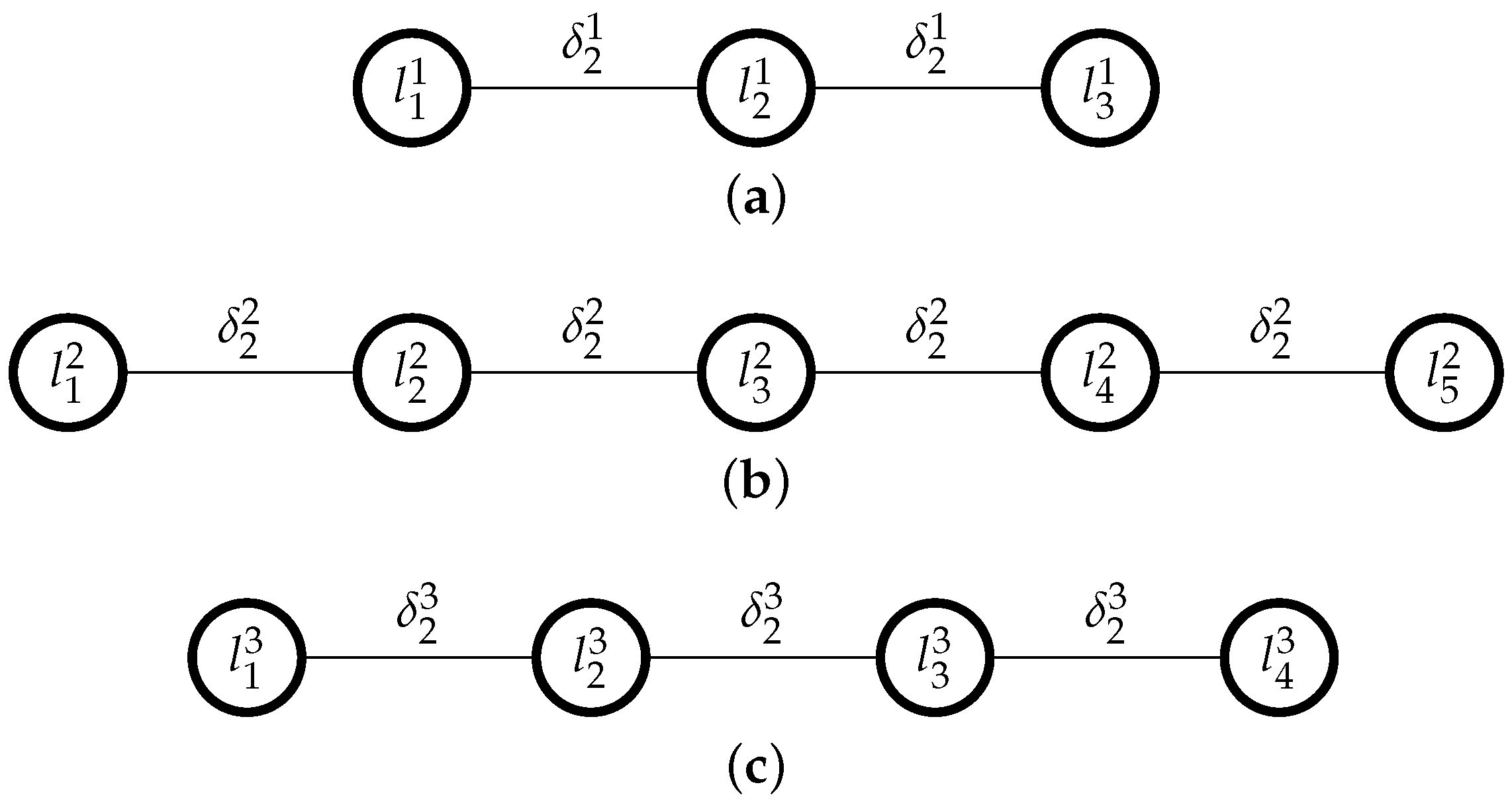
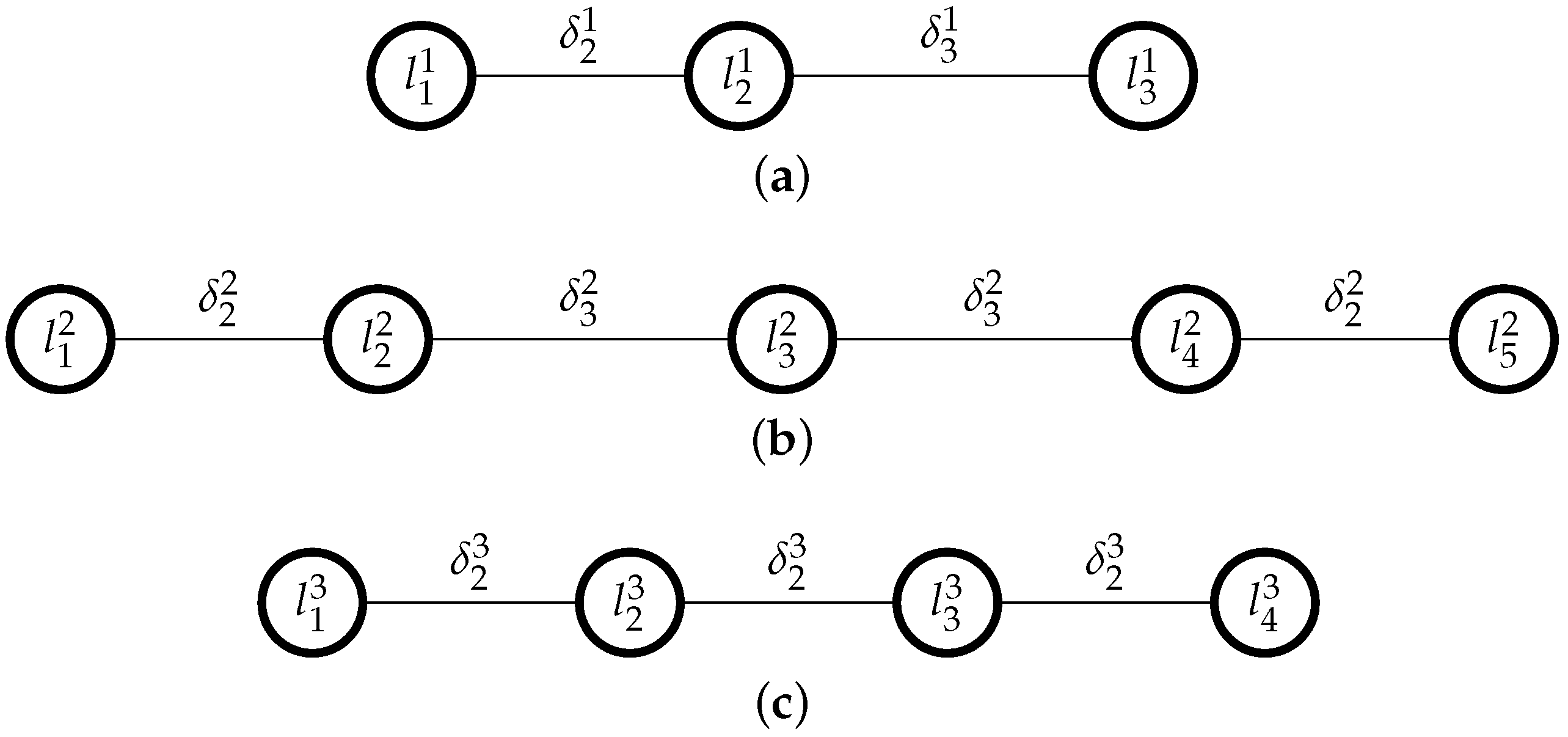
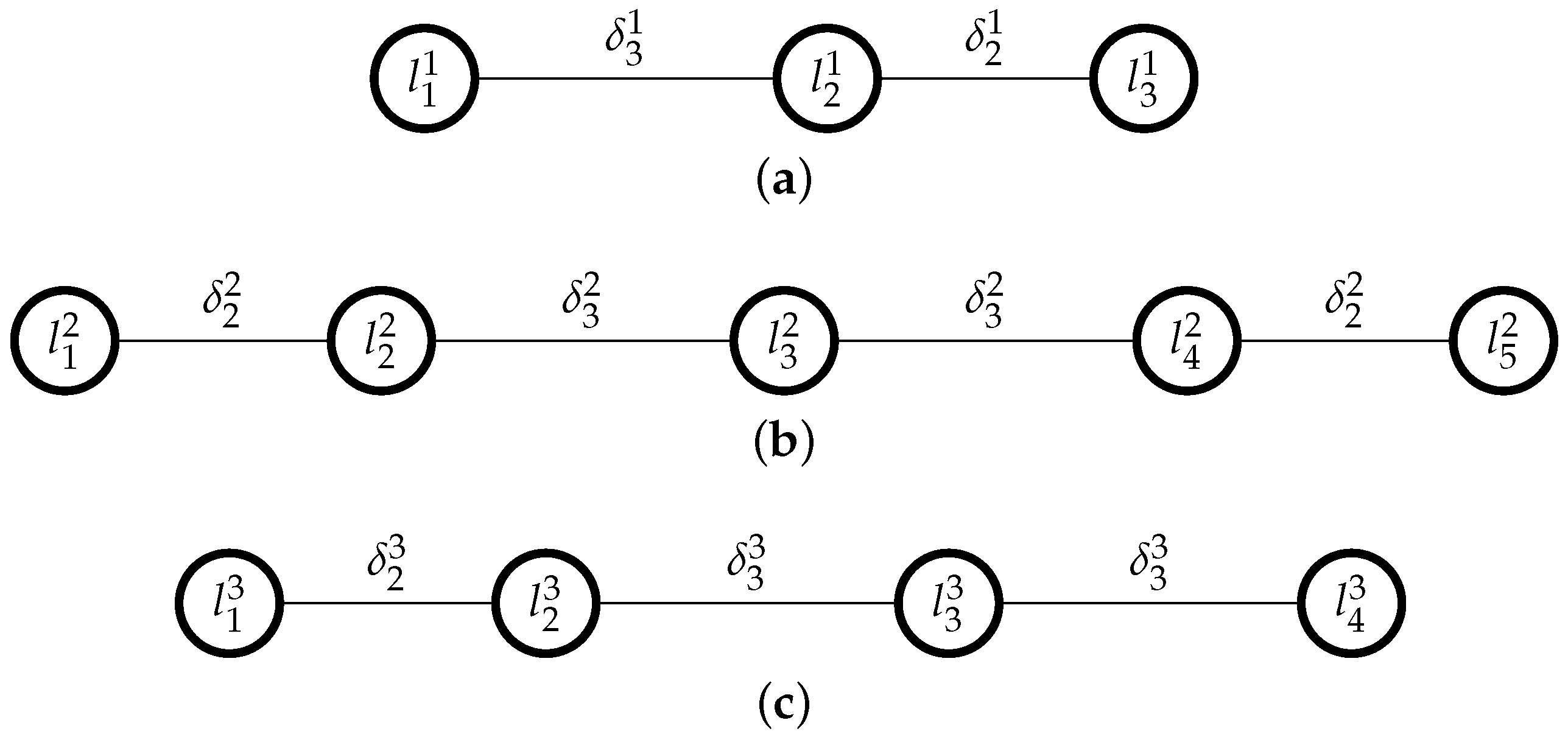
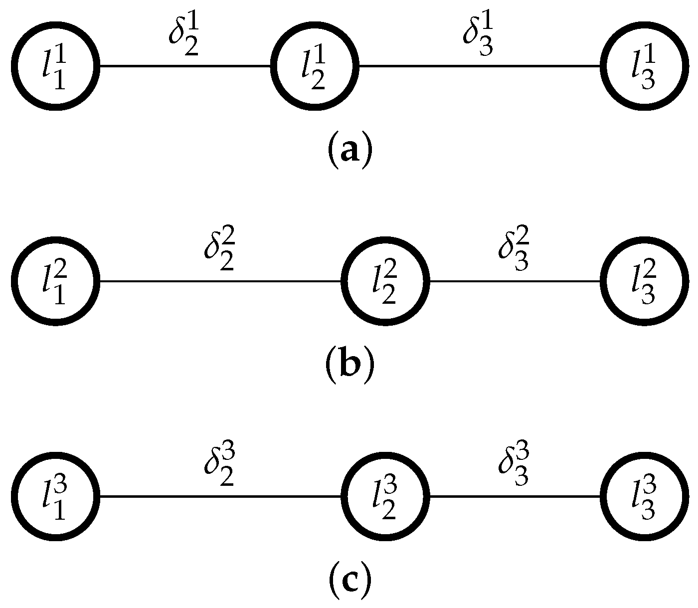
For $g=3$ there are three OPMs and all of them are metrizable. However, when $g>3$ the complexity of constructing OPMs increases. In these cases, we can apply an algorithm that generates metrizable OPMs (see García-Lapresta et al. [33]). To do that, the algorithm is based on appropriate sequences of questions whose answers lead to metrizable OPMs. For $g=4$ there are 51 OPMs, but only 25 of them are metrizable.

3. The MCDM Procedure

In this section, we present an MCDM procedure for ranking a set of alternatives $X=\{x_1,\dots ,x_n\}$, with $n\ge 2$ that are assessed by a group of agents $A=\{a_1,\dots ,a_m\}$, with $m\ge 2$, regarding a set of different criteria $C=\{c_1,\dots ,c_q\}$. MCDM authors have proposed many methods for determining criteria weights (see, for instance, Solymosi and Dombi [38], Borcherding et al. [39], Diakoulaki et al. [40], Marichal and Roubens [41], Figueira and Roy [42], and Kao [43], among others). To focus on the main ideas in this contribution, we assume that the weights are exogenously given and they are collected in a weighting vector $(w_1,\dots ,w_q)\in {[0,1]}^q$, with $w_1+\cdots +w_q=1$. This is a common situation for evaluation panels and competition juries in which the weights are given in the regulations. Nevertheless, the procedure can easily be adapted to the case in which each agent uses different weights.

Agents assess the alternatives through a specific OQS for each criterion $c_k\in C$, ${\mathcal{L}}^k=\{l_1^k,\dots ,l_{g_k}^k\}$, equipped with a metrizable OPM ${\pi }^k:{\mathcal{L}}^k\times {\mathcal{L}}^k⟶{\Delta }^k$, where ${\Delta }^k=\{{\delta }_1^k,\dots ,{\delta }_{h_k}^k\}$. To focus on the main ideas in this contribution, we assume that all agents use the same scale and the same OPMs (one for each criterion). Again, this assumption can easily be dropped. Assuming the agents have the same OPMs means that they need to agree on the ordinal proximity levels before making their assessments of the alternatives, which is an essential step to ensure they attach the same meaning to the possible grades in the scale.

The proposed procedure is related to the Copeland rule (see Copeland [44]) and to the net flow method used in PROMETHEE II (see Brans [45], Brans and Vincke [46], Bouyssou [47] and Brans and De Smet [48]). The Copeland rule is a voting system that ranks order the alternatives taking into account the number of pairwise victories minus the number of pairwise defeats. The method PROMETHEE II generates a ranking considering positive and negative flows for each alternative according to the given criteria weights. The positive flow shows how much an alternative dominates over the others (the higher the positive flow, the better the alternative). The negative flow shows the dominance of all the other alternatives over the considered one (the smaller the negative flow, the better the alternative).

The assessments provided by the agents to the alternatives with respect to the criterion $c_k$ are collected in a profile$V^k$, a matrix of m rows and n columns of linguistic terms, where $v_i^{a,k}\in {\mathcal{L}}^k$ is the assessment given by the agent a to the alternative $x_i$ regarding the criterion $c_k$:

$$V^k=\left(\begin{array}{ccccc}{v}_1^{1,k}& \cdots & v_i^{1,k}& \cdots & v_n^{1,k}\\ \cdots & \cdots & \cdots & \cdots & \cdots \\ v_1^{a,k}& \cdots & v_i^{a,k}& \cdots & v_n^{a,k}\\ \cdots & \cdots & \cdots & \cdots & \cdots \\ v_1^{m,k}& \cdots & v_i^{m,k}& \cdots & v_n^{m,k}\end{array}\right).$$

3.1. The Procedure

To rank the alternatives, the procedure is divided into the following steps:

• Gather the agents’ assessments in the corresponding profiles $V^1,\dots ,V^q$.
• Calculate, for every pair of alternatives $x_i,x_j\in X$, the ordinal degrees of proximity between the assessments given by the agents, ${\pi }^k\left(v_i^{a,k},v_j^{a,k}\right)$, for all $a\in A$ and $c_k\in C$.
• Homogenize the ordinal degrees of proximity coming from the metrizable OPMs considered in the different criteria by means of a mapping $\rho :{\bigcup }_{k=1}^q{\Delta }^k⟶[0,1]$. Such mapping $\rho$ must satisfy the following conditions for every $k\in \{1,\dots ,q\}$:
  • Min-normalization: $\rho \left({\delta }_1^k\right)=0$.
  • Max-normalization: $\rho \left({\delta }_{h_k}^k\right)=1$.
  • Strict monotonicity: $\rho \left({\delta }_{r+1}^k\right)>\rho \left({\delta }_r^k\right)$, $\forall r\in \{1,\dots ,h_k-1\}$.
• Assign a score to the alternatives, through the mapping $S:X⟶\mathbb{R}$ defined as

  $$\begin{array}{ccc}\hfill S\left(x_i\right)& =& \sum _{a=1}^m\sum _{\begin{array}{c}k=1\\ v_i^{a,k}\succ v_j^{a,k}\end{array}}^q{w}_k·\rho \left({\pi }^k\left(v_i^{a,k},v_j^{a,k}\right)\right)-\hfill \\ & & \sum _{a=1}^m\sum _{\begin{array}{c}k=1\\ v_i^{a,k}\prec v_j^{a,k}\end{array}}^q{w}_k·\rho \left({\pi }^k\left(v_i^{a,k},v_j^{a,k}\right)\right).\hfill \end{array}$$

  (1)

  Following the approaches of the Copeland rule and the PROMETHEE II, $S\left(x_i\right)$ is divided into two parts. The first part of Equation (1) considers, for the criterion k and for the agent a, the victories of the linguistic assessment $v_i^{a,k}$ over the rest of assessments $v_j^{a,k}$ (the higher, the better), and the second part the defeats of the linguistic assessment $v_i^{a,k}$ over the rest of assessments $v_j^{a,k}$ (the lower, the better).
  In Equation (1), ${\pi }^k\left(v_i^{a,k},v_j^{a,k}\right)$ measures for the criterion k and for the agent a, the proximity between the assessments $v_i^{a,k}$ and $v_j^{a,k}$. By means of these ordinal degrees of proximity, $S\left(x_i\right)$ considers the scope of victories and defeats. The mapping $\rho$ converts the ordinal degrees of proximity to the interval [0,1]. Then, the final score is calculated multiplying the obtained results by the corresponding weights.
• Order the alternatives through the weak order ⪰ on X:

  $$x_i⪰x_j\iff S\left(x_i\right)\ge S\left(x_j\right).$$

We now enumerate some properties that the proposed procedure satisfies:

• Anonymity: All agents are treated equally by the procedure.
• Neutrality: All alternatives are treated equally by the procedure.
• Monotonicity: If an agent improves the evaluation of an alternative on some criterion, all else remaining equal, then its score increases.
• Cancelation: In the uniform case, when two agents a and b increase and decrease at the same time their assessments, in such a way that agent a increases the assessment $v_i^{a,k}=l_r$ to $l_{r+1}$ and agent b decreases the assessment $v_i^{b,k}=l_r$ to $l_{r-1}$, for some alternative $x_i$ and criterion $c_k$, then $S\left(x_i\right)$ does not change.

Definition 4.

Given a metrizable OPM $\pi :\mathcal{L}\times \mathcal{L}⟶\Delta$, ρ preserves OPM linearity if $\rho \left({\pi }_{rt}\right)=\rho \left({\pi }_{rs}\right)+\rho \left({\pi }_{st}\right)$, for all $r,s,t\in \{1,\dots ,g\}$ such that $r<s<t$.

Remark 1.

If ρ preserves OPM linearity, then one can interpret the proximities between levels as the difference of proximities between such levels and the worst performance as follows:

$$\rho \left({\pi }^k(v_i^{a,k},v_j^{a,k})\right)=\left\{\begin{array}{cc}\rho \left({\pi }^k(l_1^k,v_i^{a,k})\right)-\rho \left({\pi }^k(l_1^k,v_j^{a,k})\right),& if{v}_i^{a,k}⪰v_j^{a,k},\\ \rho \left({\pi }^k(l_1^k,v_j^{a,k})\right)-\rho \left({\pi }^k(l_1^k,v_i^{a,k})\right),& if{v}_i^{a,k}\prec v_j^{a,k}.\end{array}\right.$$

Moreover, this allows rewriting Equation (1) as:

$$\begin{array}{c}S\left(x_i\right)=\sum _{a=1}^m\sum _{\begin{array}{c}k=1\\ v_i^{a,k}\succ v_j^{a,k}\end{array}}^q{w}_k·\left(\rho \left({\pi }^k(l_1^k,v_i^{a,k})\right)-\rho \left({\pi }^k(l_1^k,v_j^{a,k})\right)\right)-\hfill \\ \sum _{a=1}^m\sum _{\begin{array}{c}k=1\\ v_i^{a,k}\prec v_j^{a,k}\end{array}}^q{w}_k·\left(\rho \left({\pi }^k(l_1^k,v_j^{a,k})\right)-\rho \left({\pi }^k(l_1^k,v_i^{a,k})\right)\right)=\hfill \\ \sum _{a=1}^m\left(n·\sum _{k=1}^q{w}_k·\rho \left({\pi }^k(l_1^k,v_i^{a,k})\right)-\sum _{\begin{array}{c}k=1\end{array}}^q\sum _{\begin{array}{c}j=1\end{array}}^n{w}_k·\rho \left({\pi }^k(l_1^k,v_j^{a,k})\right)\right).\hfill \end{array}$$

(2)

Since the rightmost summation is a constant that does not depend on $x_i$, if $\rho$ preserves OPM linearity then its overall evaluation depends only on

$$\sum _{a=1}^m\sum _{k=1}^q{w}_k·\rho \left({\pi }^k(l_1^k,v_i^{a,k})\right).$$

(3)

Remark 2.

The simplest mapping considers that consecutive qualitative levels on a given criterion always represent the same difference, as follows:

$$\rho \left({\delta }_r^k\right)=\frac{r-1}{h_k-1}.$$

(4)

This mapping preserves OPM linearity if the OPM is uniform, but not in the general case.

3.2. Linear Programming Formulation

A linear program can be solved to obtain a $\rho$ mapping that preserves OPM linearity. The following formulation does so by maximizing the minimum difference between consecutive levels, i.e.,

$$max\underset{r=2,\dots ,h_k}{min}\left(\rho \left({\delta }_r^k\right)-\rho \left({\delta }_{r-1}^k\right)\right).$$

This can be formulated as a linear program by introducing an auxiliary variable $\sigma$.

To simplify notation, let ${\rho }_{r,s}^k$ denote $\rho \left({\pi }_{rs}^k\right)$. The main decision variables are the $\rho$ variables corresponding to the consecutive levels, ${\rho }_{1,2}^k$, ${\rho }_{2,3}^k$,…, ${\rho }_{g_k-1,g_k}^k$, plus the auxiliary variable $\sigma$.

Linear Program:

$$\begin{array}{cc}\hfill & max\sigma \hfill \\ \hfill & \mathrm{subject} \mathrm{to}:\hfill \\ \hfill & \sum _{r=c-1}^c{\rho }_{r-1,r}^k={\rho }_{c-2,c}^k, \mathrm{for} c=3,\dots ,g_k\hfill & \hfill \left[\mathrm{C}1\right]\\ \hfill & \sum _{r=c-2}^c{\rho }_{r-1,r}^k={\rho }_{c-3,c}^k, \mathrm{for} c=4,\dots ,g_k\hfill & \hfill \left[\mathrm{C}2\right]\\ \hfill & \dots \hfill \\ \hfill & \sum _{r=2}^{g_k}{\rho }_{r-1,r}^k={\rho }_{1,g_k}^k=1\hfill & \hfill \left[\mathrm{C}3\right]\\ \hfill & {\rho }_{r,s}^k={\rho }_{t,u}^k,\forall r,s,t,u:r>s\wedge t>u\wedge {\pi }_{rs}^k={\pi }_{tu}^k\hfill & \hfill \left[\mathrm{C}4\right]\\ \hfill & {\rho }_{r,s}^k\ge {\rho }_{t,u}^k+\sigma ,\forall r,s,t,u:r>s\wedge t>u\wedge {\pi }_{rs}^k>{\pi }_{tu}^k\hfill & \hfill \left[\mathrm{C}5\right]\\ \hfill & {\rho }_{r,s}^k\le {\rho }_{t,u}^k-\sigma ,\forall r,s,t,u:r>s\wedge t>u\wedge {\pi }_{rs}^k<{\pi }_{tu}^k\hfill & \hfill \left[\mathrm{C}6\right]\\ \hfill & {\rho }_{r-1,r}^k\ge \sigma , \mathrm{for} r=2,\dots ,g_k\hfill & \hfill \left[\mathrm{C}7\right]\end{array}$$

In this linear program, the first group of constraints, [C1], indicates that every subset of three consecutive levels $l_{c-2}^k$, $l_{c-1}^k$, $l_c^k$ must be such that ${\rho }_{c-2,c-1}^k+{\rho }_{c-1,c}^k={\rho }_{c-2,c}^k$; a second group of constraints, [C2], indicates that every subset of four consecutive levels $l_{c-3}^k$, $l_{c-2}^k$, $l_{c-1}^k$, $l_c^k$ must be such that ${\rho }_{c-3,c-2}^k+{\rho }_{c-2,c-1}^k+{\rho }_{c-1,c}^k={\rho }_{c-3,c}^k$, and so on, until constraint [C3]. These constraints together ensure linearity. For instance, if a scale has 5 linguistic terms $(g_k=5)$, then these linearity constraints would be: ${\rho }_{1,2}^k+{\rho }_{2,3}^k={\rho }_{1,3}^k$, ${\rho }_{2,3}^k+{\rho }_{3,4}^k={\rho }_{2,4}^k$, ${\rho }_{3,4}^k+{\rho }_{4,5}^k={\rho }_{3,5}^k$ ([C1]), ${\rho }_{1,2}^k+{\rho }_{2,3}^k+{\rho }_{3,4}^k={\rho }_{1,4}^k$, ${\rho }_{2,3}^k+{\rho }_{3,4}^k+{\rho }_{4,5}^k={\rho }_{2,5}^k$ ([C2]), and ${\rho }_{1,2}^k+{\rho }_{2,3}^k+{\rho }_{3,4}^k+{\rho }_{4,5}^k={\rho }_{1,5}^k=1$ ([C3]).

Then, constraints [C4-C6] are needed to ensure the monotonicity of the $\rho$ mapping. Constraint [C4] can be used to reduce the number of variables in the linear program. Finally, constraint [C7] requires the $\rho$ mapping to be positive.

Proposition 1.

If an OPM is uniform, then Equation (4) is an optimal solution for the above linear program.

Proof 

Given several levels $g_k$, a uniform OPM requires $h_k=g_k$ proximity degrees and Equation (4) yields $\rho \left({\delta }_1^k\right)=0$, $\rho \left({\delta }_2^k\right)=\frac{1}{g_k-1}$, $\rho \left({\delta }_3^k\right)=\frac{2}{g_k-1}$,…, $\rho \left({\delta }_{g_k}^k\right)=1$. In such OPMs, ${\pi }_{12}^k={\pi }_{23}^k$, ${\pi }_{23}^k={\pi }_{24}^k$, etc., which by constraint [C4] implies ${\rho }_{1,2}^k={\rho }_{2,3}^k$, etc. Then, constraint [C3] implies ${\sum }_{r=2}^{g_k}{\rho }_{r-1,r}^k=(g_k-1){\rho }_{1,2}^k=1$, which means that the solution provided by Equation (4) is the only one satisfying these constraints.

Moreover, ${\rho }_{c-2,c-1}^k={\rho }_{c-1,c}^k=\rho \left({\delta }_2^k\right)$ and ${\rho }_{c-2,c}^k=\rho \left({\delta }_3^k\right)=2\rho \left({\delta }_2^k\right)$, hence the constraints [C1] are satisfied. Similarly, all other linearity constraints [C2] until [C3] are naturally satisfied. Therefore, Equation (4) is a feasible solution to the linear program and, since it is the only feasible solution, it is also optimal. □

3.3. Stochastic Analysis

As mentioned before, the $\rho$ mapping can be obtained by a formula (e.g., Equation (4), which considers equal differences between any consecutive qualitative levels on a given criterion), or it can result from an optimization process enforcing linearity. However, in general there can be multiple other $\rho$ mappings preserving linearity. To analyze the results corresponding to the multiple $\rho$ mappings that preserve linearity it is possible to follow a stochastic approach, inspired by the Stochastic Multi-attribute Acceptability Analysis (SMAA) methods [36,49,50,51].

In the stochastic analysis, one samples randomly many $\rho$ mappings, and then results are computed for each of these mappings. This allows obtaining statistics about the results, such as:

• The rank acceptability indices $r_i^p$ (for each alternative $x_i$, for each ranking position p), which is the probability (in terms or relative frequency) that alternative $x_i$ is ranked in position p ($i,p=1,\dots ,n$).
• The pairwise winning indices $p(i,j)$ (for each pair of alternatives $(x_i,x_j)$), which is the probability (in terms or relative frequency) that alternative $x_i$ is ranked better than $x_j$ ($i,j=1,\dots ,n$).

To generate a random $\rho$ mapping preserving linearity it is sufficient to generate randomly the $\rho$ values corresponding to the differences in the consecutive levels ${\rho }_{1,2}^k$, ${\rho }_{2,3}^k$,…, ${\rho }_{g_k-1,g_k}^k$. In one extreme case, when the consecutive levels are all different, the number of random numbers to generate is equal to $g_k-1$. In the other extreme case, when the consecutive levels are all equal, no random number needs to be generated. The needed random numbers can be sorted from lowest to highest and assigned in this order to the ${\pi }_{i,i+1}^k$, from the lowest to the highest corresponding ${\pi }_{i,i+1}^k$. When needed, a hit-and-run approach [50] can be followed to exclude cases in which the $\rho$ values obtained by summing the obtained numbers do not respect the ordinal relation between the remaining ${\pi }_{rs}^k$. For the cases in which the ordinal relations are respected, the generated random values can be divided by the sum ${\rho }_{1,2}^k+{\rho }_{2,3}^k+\cdots +{\rho }_{g_k-1,g_k}^k$ to normalize this sum to unity.

4. Practical Applications

To show how the proposed procedure works, we present an illustrative example that considers different proximities between the terms of OQSs. We also introduce a stochastic approach to assess the robustness of the conclusions obtained. Lastly, we apply our procedure to rank a selection of Research and Development (R&D) projects and compare its results with the ones obtained applying the methods SMAA-O (see Lahdelma [36]) and ZAPROS III (see Larichev [37]).

4.1. An Illustrative Example

In this subsection, we apply the MCDM procedure to rank a set of alternatives. To do that, we consider three hotels which have been assessed by six agents taking into account three criteria: location, comfort of the rooms and service.

Table 1. OQSs for each criterion.

Location			Rooms			Service
$l_1^1$	Poor		$l_1^2$	Very uncomfortable		$l_1^3$	Poor
$l_2^1$	Acceptable		$l_2^2$	Somewhat uncomfortable		$l_2^3$	Fair
$l_3^1$	Good		$l_3^2$	Neither comfortable nor uncomfortable		$l_3^3$	Good
			$l_4^2$	Somewhat comfortable		$l_4^3$	Excellent
			$l_5^2$	Very comfortable

shows the OQSs used for evaluating each criterion. To determine the criteria weights in hotel selection, we consider an empirical study where the most important criteria are those related to rooms such as: comfort and equipment of rooms, followed by the service and location (see Zaman et al. [52]). The different weights associated with each criterion are presented in

Table 2. Weights for each criterion.

Weights
$w_1$	0.20
$w_2$	0.50
$w_3$	0.30

and the assessments given by the agents over the hotels are collected in

Table 3. Linguistic assessments given by the agents.

	Hotel 1	Hotel 2	Hotel 3			Hotel 1	Hotel 2	Hotel 3
Location	$l_2^1$	$l_3^1$	$l_2^1$		Location	$l_3^1$	$l_2^1$	$l_2^1$
Rooms	$l_4^2$	$l_5^2$	$l_3^2$		Rooms	$l_5^2$	$l_4^2$	$l_4^2$
Service	$l_2^3$	$l_1^3$	$l_3^3$		Service	$l_4^3$	$l_3^3$	$l_3^3$
Assessments given by the agent 1.					Assessments given by the agent 2.
	Hotel 1	Hotel 2	Hotel 3			Hotel 1	Hotel 2	Hotel 3
Location	$l_1^1$	$l_2^1$	$l_3^1$		Location	$l_2^1$	$l_3^1$	$l_3^1$
Rooms	$l_5^2$	$l_3^2$	$l_5^2$		Rooms	$l_3^2$	$l_3^2$	$l_4^2$
Service	$l_1^3$	$l_2^3$	$l_3^3$		Service	$l_2^3$	$l_3^3$	$l_3^3$
Assessments given by the agent 3.					Assessments given by the agent 4.
	Hotel 1	Hotel 2	Hotel 3			Hotel 1	Hotel 2	Hotel 3
Location	$l_2^1$	$l_3^1$	$l_2^1$		Location	$l_3^1$	$l_3^1$	$l_3^1$
Rooms	$l_3^2$	$l_4^2$	$l_2^2$		Rooms	$l_4^2$	$l_5^2$	$l_3^2$
Service	$l_4^3$	$l_3^3$	$l_3^2$		Service	$l_3^3$	$l_1^3$	$l_3^3$
Assessments given by the agent 5.					Assessments given by the agent 6.

.

To illustrate the proposed procedure, we consider three different cases. First, the uniform case; and then, two non-uniform cases.

4.1.1. The Uniform Case

The uniform case considers the metrizable OPMs ${\pi }^1,{\pi }^2$ and ${\pi }^3$ associated with the proximity matrices $A_{22}$, $A_{2222}$ and $A_{222}$:

$$A_{22}=\left(\begin{array}{ccc}{\delta }_1^1& {\delta }_2^1& {\delta }_3^1\\ & {\delta }_1^1& {\delta }_2^1\\ & & {\delta }_1^1\end{array}\right),A_{2222}=\left(\begin{array}{ccccc}{\delta }_1^2& {\delta }_2^2& {\delta }_3^2& {\delta }_4^2& {\delta }_5^2\\ & {\delta }_1^2& {\delta }_2^2& {\delta }_3^2& {\delta }_4^2\\ & & {\delta }_1^2& {\delta }_2^2& {\delta }_3^2\\ & & & {\delta }_1^2& {\delta }_2^2\\ & & & & {\delta }_1^2\end{array}\right),$$

$$A_{222}=\left(\begin{array}{cccc}{\delta }_1^3& {\delta }_2^3& {\delta }_3^3& {\delta }_4^3\\ & {\delta }_1^3& {\delta }_2^3& {\delta }_3^3\\ & & {\delta }_1^3& {\delta }_2^3\\ & & & {\delta }_1^3\end{array}\right)$$

that can be visualized in Figure 1. The subindices of the matrices $A^{\prime }s$ correspond to the subindices of the ${\delta }^{\prime }s$ appearing in the coefficients just over the main diagonal. We follow this pattern to denote subsequent matrices.

Table 4. $\delta$ values obtained for hotel 1. Uniform case.

		Agent 1			Agent 2			Agent 3
		${\mathit{v}}_{\mathit{i}}$	${\mathit{v}}_{\mathit{j}}$	$\mathit{\pi }({\mathit{v}}_{\mathit{i}},{\mathit{v}}_{\mathit{j}})$	${\mathit{v}}_{\mathit{i}}$	${\mathit{v}}_{\mathit{j}}$	$\mathit{\pi }({\mathit{v}}_{\mathit{i}},{\mathit{v}}_{\mathit{j}})$	${\mathit{v}}_{\mathit{i}}$	${\mathit{v}}_{\mathit{j}}$	$\mathit{\pi }({\mathit{v}}_{\mathit{i}},{\mathit{v}}_{\mathit{j}})$
H1 vs. H2	Location	$l_2^1$	$l_3^1$	${\delta }_2$	$l_3^1$	$l_2^1$	${\delta }_2$	$l_1^1$	$l_2^1$	${\delta }_2$
	Rooms	$l_4^2$	$l_5^2$	${\delta }_2$	$l_5^2$	$l_4^2$	${\delta }_2$	$l_5^2$	$l_3^2$	${\delta }_3$
	Service	$l_2^3$	$l_1^3$	${\delta }_2$	$l_4^3$	$l_3^3$	${\delta }_2$	$l_1^3$	$l_2^3$	${\delta }_2$
H1 vs. H3	Location	$l_2^1$	$l_2^1$	${\delta }_1$	$l_3^1$	$l_2^1$	${\delta }_2$	$l_1^1$	$l_3^1$	${\delta }_3$
	Rooms	$l_4^2$	$l_3^2$	${\delta }_2$	$l_5^2$	$l_4^2$	${\delta }_2$	$l_5^2$	$l_5^2$	${\delta }_1$
	Service	$l_2^3$	$l_3^3$	${\delta }_2$	$l_4^3$	$l_3^3$	${\delta }_2$	$l_1^3$	$l_3^3$	${\delta }_3$
		Agent 4			Agent 5			Agent 6
		${\mathit{v}}_{\mathit{i}}$	${\mathit{v}}_{\mathit{j}}$	$\mathit{\pi }({\mathit{v}}_{\mathit{i}},{\mathit{v}}_{\mathit{j}})$	${\mathit{v}}_{\mathit{i}}$	${\mathit{v}}_{\mathit{j}}$	$\mathit{\pi }({\mathit{v}}_{\mathit{i}},{\mathit{v}}_{\mathit{j}})$	${\mathit{v}}_{\mathit{i}}$	${\mathit{v}}_{\mathit{j}}$	$\mathit{\pi }({\mathit{v}}_{\mathit{i}},{\mathit{v}}_{\mathit{j}})$
H1 vs. H2	Location	$l_2^1$	$l_3^1$	${\delta }_2$	$l_2^1$	$l_3^1$	${\delta }_2$	$l_3^1$	$l_3^1$	${\delta }_1$
	Rooms	$l_3^2$	$l_3^2$	${\delta }_1$	$l_3^2$	$l_4^2$	${\delta }_2$	$l_4^2$	$l_5^2$	${\delta }_2$
	Service	$l_2^3$	$l_3^3$	${\delta }_2$	$l_4^3$	$l_3^3$	${\delta }_2$	$l_3^3$	$l_1^3$	${\delta }_3$
H1 vs. H3	Location	$l_2^1$	$l_3^1$	${\delta }_2$	$l_2^1$	$l_2^1$	${\delta }_1$	$l_3^1$	$l_3^1$	${\delta }_1$
	Rooms	$l_3^2$	$l_4^2$	${\delta }_2$	$l_3^2$	$l_2^2$	${\delta }_2$	$l_4^2$	$l_3^2$	${\delta }_2$
	Service	$l_2^3$	$l_3^3$	${\delta }_2$	$l_4^3$	$l_3^3$	${\delta }_2$	$l_3^3$	$l_3^3$	${\delta }_1$

shows for Hotel 1 the $\pi$ values obtained taking into account the above metrizable OPMs and the linguistic assessments contained in Table 3.

After applying the procedure to Hotel 1 produces the following results:

Location:

$$0.20·\left({\displaystyle -\frac{1}{2}+\frac{1}{2}-\frac{1}{2}-\frac{1}{2}-\frac{1}{2}+0+0+\frac{1}{2}-\frac{2}{2}-\frac{1}{2}+0+0}\right)=-0.50.$$

Rooms:

$$0.50·\left({\displaystyle -\frac{1}{4}+\frac{1}{4}+\frac{2}{4}+0-\frac{1}{4}-\frac{1}{4}+\frac{1}{4}+\frac{1}{4}+0-\frac{1}{4}+\frac{1}{4}+\frac{1}{4}}\right)=0.375.$$

Service:

$$0.30·\left({\displaystyle \frac{1}{3}+\frac{1}{3}-\frac{1}{3}-\frac{1}{3}+\frac{1}{3}+\frac{2}{3}-\frac{1}{3}+\frac{1}{3}-\frac{2}{3}-\frac{1}{3}+\frac{1}{3}+0}\right)=0.10.$$

Thus, for Hotel 1 we obtain $S\left(H_1\right)=-0.5+0.375+0.10=-0.025$.

After applying the procedure to Hotels 2 and 3, we have $S\left(H_2\right)=-0.025$ and $S\left(H_3\right)=0.05$. Then, Hotel 3 ≻ Hotel 1 ∼ Hotel 2.

4.1.2. A Non-Uniform Case 1

In this case, we continue taking into account the same OPM, $A_{222}$, for the third scale contained in Table 1. However, we consider two different ways to devise the other scales. These latter scales are equipped with the metrizable OPMs associated with the proximity matrices $A_{23}$, $A_{2332}$:

$$A_{23}=\left(\begin{array}{ccc}{\delta }_1^1& {\delta }_2^1& {\delta }_4^1\\ & {\delta }_1^1& {\delta }_3^1\\ & & {\delta }_1^1\end{array}\right),A_{2332}=\left(\begin{array}{ccccc}{\delta }_1^2& {\delta }_2^2& {\delta }_4^2& {\delta }_6^2& {\delta }_7^2\\ & {\delta }_1^2& {\delta }_3^2& {\delta }_5^2& {\delta }_6^2\\ & & {\delta }_1^2& {\delta }_3^2& {\delta }_4^2\\ & & & {\delta }_1^2& {\delta }_2^2\\ & & & & {\delta }_1^2\end{array}\right),$$

$$A_{222}=\left(\begin{array}{cccc}{\delta }_1^3& {\delta }_2^3& {\delta }_3^3& {\delta }_4^3\\ & {\delta }_1^3& {\delta }_2^3& {\delta }_3^3\\ & & {\delta }_1^3& {\delta }_2^3\\ & & & {\delta }_1^3\end{array}\right)$$

that can be visualized in Figure 2.

After applying the procedure, we obtain $S\left(H_1\right)=-0.017$, $S\left(H_2\right)=0.083$ and $S\left(H_3\right)=-0.067$. Then, Hotel 2 ≻ Hotel 1 ≻ Hotel 3.

4.1.3. A Non-Uniform Case 2

In this second case we consider that the three OQSs are not uniform. The scales are equipped with the metrizable OPMs associated with the following proximity matrices $A_{32}$, $A_{2332}$ and $A_{233}$:

$$A_{32}=\left(\begin{array}{ccc}{\delta }_1^1& {\delta }_3^1& {\delta }_4^1\\ & {\delta }_1^1& {\delta }_2^1\\ & & {\delta }_1^1\end{array}\right),A_{2332}=\left(\begin{array}{ccccc}{\delta }_1^2& {\delta }_2^2& {\delta }_4^2& {\delta }_6^2& {\delta }_7^2\\ & {\delta }_1^2& {\delta }_3^2& {\delta }_5^2& {\delta }_6^2\\ & & {\delta }_1^2& {\delta }_3^2& {\delta }_4^2\\ & & & {\delta }_1^2& {\delta }_2^2\\ & & & & {\delta }_1^2\end{array}\right),$$

$$A_{233}=\left(\begin{array}{cccc}{\delta }_1^3& {\delta }_2^3& {\delta }_4^3& {\delta }_6^3\\ & {\delta }_1^3& {\delta }_3^3& {\delta }_5^3\\ & & {\delta }_1^3& {\delta }_3^3\\ & & & {\delta }_1^3\end{array}\right).$$

The OPMs considered in the non-uniform case 2 can be visualized in Figure 3.

When we apply the proposed procedure, we obtain the following results: $S\left(H_1\right)=0.07$, $S\left(H_2\right)=-0.03$ and $S\left(H_3\right)=-0.04$. Then, Hotel 1 ≻ Hotel 2 ≻ Hotel 3.

Table 5. Results obtained in the three cases.

The Uniform Case	Non-Uniform Case 1	Non-Uniform Case 2
Hotel 3	Hotel 2	Hotel 1
Hotel 1    Hotel 2	Hotel 1	Hotel 2
	Hotel 3	Hotel 3

summarizes the results obtained after applying the procedure in the three cases considered. As can be seen, the rankings of the three hotels are different depending on how the proximities between the terms of the scales are perceived. This makes it extremely important that the agents debate which OPM best matches their interpretation of the linguistic terms, so that if proximities are not uniform then an appropriate non-uniform OPM is used instead.

4.1.4. Stochastic Analysis of the Non-Uniform Case 2

To illustrate the use of the stochastic analysis (Section 3.3), let us consider the non-uniform case 2 (Section 4.1.3). As depicted in Figure 3, for each scale only two random numbers need to be drawn: one to represent $\rho \left({\delta }_2^k\right)$ and another one to represent $\rho \left({\delta }_3^k\right)$ (values are drawn independently for each scale). These numbers are normalized dividing them by $\rho \left({\delta }_2^1\right)+\rho \left({\delta }_2^1\right)$ in the case of $A_{32}$, dividing them by $2·\rho \left({\delta }_2^2\right)+2·\rho \left({\delta }_2^2\right)$ in the case of $A_{2332}$, and dividing them by $\rho \left({\delta }_2^3\right)+2·\rho \left({\delta }_2^3\right)$ in the case of $A_{233}$. All other ordinality constraints are respected (e.g., $\rho \left({\delta }_5^3\right)$ is surely greater than $\rho \left({\delta }_4^3\right)$ because $\rho \left({\delta }_3^3\right)+\rho \left({\delta }_3^3\right)>\rho \left({\delta }_2^3\right)+\rho \left({\delta }_3^3\right)$). The sampling was performed by running 10 000 iterations in a Monte-Carlo simulation.

Table 6. Rank acceptability indices: probability of attaining each ranking position.

Alternative	Rank 1 (Best)	Rank 2	Rank 3
Hotel 1	0.892	0.108	0
Hotel 2	0	0.543	0.457
Hotel 3	0.108	0.349	0.543

presents the rank acceptability indices for the three alternatives. Hotel 1 wins most of the times and is never ranked third (null acceptability for rank 3), whereas Hotel 2 never wins but nevertheless stays in the second position more often than in the third. Hotel 3 can be placed in any of the three positions, although it only reached the best position in less than 11% of the cases and its most likely position is the worst one.

These results can be further clarified by observing the pairwise winning indices on

Table 7. Pairwise winning indices: probability of row alternative being better than column alternative.

	Hotel 1	Hotel 2	Hotel 3
Hotel 1	-	1.00	0.892
Hotel 2	0.00	-	0.543
Hotel 3	0.108	0.457	-

. It is possible to see why Hotel 2 cannot win: Hotel 1 beat it in all the simulations. The few cases in which Hotel 1 does not win correspond to the cases in which it is beaten by Hotel 3. This analysis indicates that in this example, the choice of Hotel 1, as indicated in the right column of Table 5, is fairly robust to changes in the definition of the $\rho$ mapping. However, the conclusion that Hotel 2 is the second best one is less robust.

These results can be compared to the results that SMAA-O [36] would provide for the same data. SMAA-O is a stochastic approach for ordinal data that samples values compatible with an ordinal scale of g levels in a straightforward way: level $l_1$ corresponds to value 0; level $l_g$ corresponds to value 1; levels $l_2$ to $l_{g-1}$ are assigned to $g-2$ random values in ascending order. A uniform distribution in [0,1] is used for this purpose.

Applying SMAA-O to this case yields the results presented in

Table 8. Rank acceptability indices according to SMAA-O.

Alternative	Rank 1 (Best)	Rank 2	Rank 3
Hotel 1	0.340	0.486	0.174
Hotel 2	0.321	0.263	0.416
Hotel 3	0.339	0.251	0.410

and

Table 9. Pairwise winning indices according to SMAA-O.

	Hotel 1	Hotel 2	Hotel 3
Hotel 1	-	0.569	0.517
Hotel 2	0.431	-	0.501
Hotel 3	0.483	0.499	-

.

Without the ability to exploit the knowledge of the ordinal proximities between the levels associated with each criterion, SMAA-O is not able to point any alternative as being the best one. Indeed, SMAA-O does not place any constraints on the mapping of qualitative scales other than respecting their order, which in this case as in many other ones is insufficient to make a clear distinction between the alternatives. Thus, when the decision makers define the criteria OPMs, the stochastic approach proposed in this paper is preferable.

4.2. Application of the Proposed MCDM Procedure to a Project Selection

In this subsection, we apply the proposed MCDM procedure to rank a selection of R&D projects and compare its results with the ones obtained applying the method ZAPROS III (see Larichev [37]). ZAPROS III belongs to the family of verbal decision analysis methods, which are applied to problems that use qualitative factors, especially difficult for formalization and numerical measurement.

Following the example presented by Larichev [37], we consider a decision maker that evaluates nine R&D projects regarding three different criteria. The OQSs used for evaluating the criteria are shown in

Table 10. Criteria and OQSs for evaluating the R&D projects.

Originality			Prospects			Qualification of the Applicant
$l_1^1$	Further development of previous ideas		$l_1^2$	Success is hardly probable		$l_1^3$	Unknown
$l_2^1$	There are new elements in the proposal		$l_2^2$	Success is rather probable		$l_2^3$	Normal
$l_3^1$	Absolutely new idea and/or approach		$l_3^2$	High probability of success		$l_3^3$	High

. Although the three criteria have three levels, the OQSs are completely different and therefore it would be a strong assumption to use the same OPM for all these criteria. The assessments given by the decision maker to the projects are collected in

Table 11. Linguistic assessments for each criterion.

	Originality	Prospects	Qualification
$x_1$	$l_3^1$	$l_2^2$	$l_2^3$
$x_2$	$l_2^1$	$l_2^2$	$l_3^3$
$x_3$	$l_1^1$	$l_3^2$	$l_2^3$
$x_4$	$l_3^1$	$l_1^2$	$l_3^3$
$x_5$	$l_2^1$	$l_3^2$	$l_1^3$
$x_6$	$l_1^1$	$l_2^2$	$l_2^3$
$x_7$	$l_1^1$	$l_2^2$	$l_3^3$
$x_8$	$l_1^1$	$l_1^2$	$l_3^3$
$x_9$	$l_2^1$	$l_3^2$	$l_2^3$

.

The method ZAPROS III constructs a partial order over the set of the alternatives. ZAPROS III is based on elicitation of preferences around values that represent distances between the assessments on the ordinal scales of two criteria. However, this method does not use a specific weight for each criterion and does not consider the proximity between the linguistic terms of the scales.

To illustrate our procedure and compare its result with the output of ZAPROS III, we assume that all criteria have the same importance and consider in each criterion the following metrizable OPMs associated with the matrix $A_{23}$, $A_{32}$ and $A_{32}$, respectively (see Figure 4).

Figure 5 shows the partial order of the projects obtained through the method ZAPROS III, and in

Table 12. Rank of the projects applying the proposed MCDM procedure.

Proposed Procedure
$x_1$
$x_9$
$x_2$$x_4$
$x_3$$x_7$
$x_5$
$x_6$
$x_8$

the results obtained after applying the proposed MCDM procedure.

The results of the procedure presented in this paper are not directly comparable with ZAPROS as these methods follow a different logic. It is noteworthy that results are in agreement concerning which are the best alternatives ($x_1$ and $x_9$) and also concerning which are the worst alternatives ($x_5$, $x_6$ and $x_8$). Nevertheless, some differences can be highlighted. The first one is that our procedure always yields a weak order, whereas ZAPROS III finds some alternatives are not comparable (e.g., $x_2$ vs $x_3$), i.e., it can yield a partial order. Another important difference can be found in the comparison of the two top contenders, $x_1$ and $x_9$. Without the ability to exploit information about ordinal proximities, ZAPROS III places $x_9$ better than $x_1$. By exploiting the information contained in the OPMs, our approach places $x_1$ better than $x_9$. Given the OPMs in Figure 4 (for different OPMs the result changes), their proximity in Originality (advantage of $x_1$) is less (i.e., they are more distant) than the proximity in Prospects (the Qualification level being equal). Therefore, it is natural to conclude $x_1$ is preferred to $x_9$.

5. Concluding Remarks

The main contribution of this paper is to provide a MCDM procedure for ranking alternatives assessed by a group of agents regarding multiple criteria through several OQSs, which can use different terms and even have different number of levels. To illustrate how the MCDM procedure works, we have ranked a set of hotels considering different proximities between the terms of the OQSs. We have also introduced a stochastic approach to assess the robustness of the conclusions.

It is important to mention that the MCDM procedure presents some advantages with respect to other proposals that deal with qualitative information:

• The proposed procedure is developed in a multi-criteria setting where alternatives are assessed by means of a specific OQS for each criterion. This is an important difference regarding other MCDM procedures that use the same qualitative scale in all criteria.
• The procedure preserves and respects ordinal information of the OQSs by means of the concept of ordinal proximity measure that takes into account how agents perceive the proximities between the linguistic terms of the scales.
• The possibility of applying the procedure in real decision-making problems such as: clinical diagnosis, quality control, customer satisfaction measurement, etc.

Regarding future research, it could be interesting to extend the proposed procedure to an uncertainty context, where agents are allowed to express their assessment by means of several consecutive linguistic terms instead of a single linguistic term (see García-Lapresta and González del Pozo [35]).

References

1. Delgado, M.; Herrera, F.; Herrera-Viedma, E.; Martínez, L. Combining numerical and linguistic information in group decision making. Inf. Sci. 1998, 107, 177–194. [Google Scholar] [CrossRef]
2. Herrera, F.; Herrera-Viedma, E.; Martínez, L. A fusion approach for managing multi-granularity linguistic term sets in decision making. Fuzzy Sets Syst. 2000, 114, 43–58. [Google Scholar] [CrossRef]
3. Herrera, F.; Martínez, L.; Sánchez, P.J. Managing non-homogeneous information in group decision making. Eur. J. Oper. Res. 2005, 166, 115–132. [Google Scholar] [CrossRef]
4. De Andrés, R.; García-Lapresta, J.L.; Martínez, L. A multi-granular linguistic model for management decision-making in performance appraisal. Soft Comput. 2010, 14, 21–34. [Google Scholar] [CrossRef]
5. Zadeh, L.A. The concept of a linguistic variable and its application to approximate reasoning, Part I. Inf. Sci. 1975, 8, 199–249. [Google Scholar] [CrossRef]
6. Zadeh, L.A. The concept of a linguistic variable and its application to approximate reasoning, Part II. Inf. Sci. 1975, 8, 301–357. [Google Scholar] [CrossRef]
7. Zadeh, L.A. The concept of a linguistic variable and its application to approximate reasoning, Part III. Inf. Sci. 1975, 9, 43–80. [Google Scholar] [CrossRef]
8. Zigmond, A.S.; Snaith, R.P. The hospital anxiety and depression scale. Acta Psychiatr. Scand. 1983, 67, 361–370. [Google Scholar] [CrossRef] [Green Version]
9. Zimmer, A.C. Verbal vs. numerical processing of subjective probabilities. Decis. Mak. Uncertain. 1983, 16, 159–182. [Google Scholar]
10. Zimmer, A.C. A model for the interpretation of verbal predictions. Int. J. Man-Mach. Stud. 1984, 20, 121–134. [Google Scholar] [CrossRef]
11. Windschitl, P.D.; Wells, G.L. Measuring psychological uncertainty: Verbal versus numerical methods. J. Exp. Psychol. Appl. 1996, 2, 343–364. [Google Scholar] [CrossRef]
12. Beyth-Marom, R. How probable is probable? A numerical translation of verbal probability expressions. J. Forecast. 1982, 1, 257–269. [Google Scholar] [CrossRef]
13. Wallsten, T.S.; Fillenbaum, S.; Cox, J.A. Base rate effects on the interpretations of probability and frequency expressions. J. Mem. Lang. 1986, 25, 571–587. [Google Scholar] [CrossRef]
14. Teigen, K.H. The language of uncertainty. Acta Psychol. 1988, 68, 27–38. [Google Scholar] [CrossRef]
15. Merbitz, C.; Morris, J.; Grip, J.C. Ordinal scales and foundations of misinference. Arch. Phys. Med. Rehabil. 1989, 70, 308–312. [Google Scholar] [PubMed]
16. Blair, J.; Lacy, M.G. Statistics of ordinal variation. Sociol. Methods Res. 2000, 28, 251–280. [Google Scholar] [CrossRef]
17. Franceschini, F. Advanced Quality Function Deployment; CRC Press: Boca Raton, FL, USA, 2001. [Google Scholar]
18. Bashkansky, E.; Gadrich, T. Evaluating quality measured on a ternary ordinal scale. Qual. Reliab. Eng. Int. 2008, 24, 957–971. [Google Scholar] [CrossRef]
19. Gadrich, T.; Bashkansky, E.; Zitikis, R. Assessing variation: A unifying approach for all scales of measurement. Qual. Quant. 2015, 49, 1145–1167. [Google Scholar] [CrossRef]
20. Franceschini, F.; Galetto, M.; Varetto, M. Qualitative ordinal scales: The concept of ordinal range. Qual. Eng. 2004, 16, 515–524. [Google Scholar] [CrossRef] [Green Version]
21. Stevens, S.S. On the theory of scales of measurement. Science 1946, 103, 677–680. [Google Scholar] [CrossRef]
22. Herrera, F.; Martínez, L. A 2-tuple fuzzy linguistic representation model for computing with words. IEEE Trans. Fuzzy Syst. 2000, 8, 746–752. [Google Scholar]
23. Herrera, F.; Herrera-Viedma, E.; Martínez, L. A fuzzy linguistic methodology to deal with unbalanced linguistic term sets. IEEE Trans. Fuzzy Syst. 2008, 16, 354–370. [Google Scholar] [CrossRef]
24. Wang, W.P. A fuzzy linguistic computing approach to supplier evaluation. Appl. Math. Model. 2010, 34, 3130–3141. [Google Scholar] [CrossRef]
25. Liu, P.; Jin, F. A multi-attribute group decision-making method based on weighted geometric aggregation operators of interval-valued trapezoidal fuzzy numbers. Appl. Math. Model. 2012, 36, 2498–2509. [Google Scholar] [CrossRef]
26. Xiao, Z.; Xia, S.; Gong, K.; Li, D. The trapezoidal fuzzy soft set and its application in MCDM. Appl. Math. Model. 2012, 36, 5844–5855. [Google Scholar] [CrossRef]
27. Zadeh, L.A. Key roles of information granulation and fuzzy logic in human reasoning, Concept formulation and computing with words. In Proceedings of the IEEE 5th International Fuzzy Systems 1, New Orleans, LA, USA, 11 September 1996; p. 1. [Google Scholar]
28. Li, X.; Ruan, D.; Liu, J.; Xu, Y. A linguistic-valued weighted aggregation operator to multiple attribute group decision making with quantitative and qualitative information. Int. J. Comput. Intell. Syst. 2008, 1, 274–284. [Google Scholar] [CrossRef]
29. Herrera, F.; Alonso, S.; Chiclana, F.; Herrera-Viedma, E. Computing with words in decision making: Foundations, trends and prospects. Fuzzy Optim. Decis. Mak. 2009, 8, 337–364. [Google Scholar] [CrossRef]
30. Franceschini, F.; Galetto, M.; Varetto, M. Ordered samples control charts for ordinal variables. Qual. Reliab. Eng. Int. 2005, 21, 177–195. [Google Scholar] [CrossRef] [Green Version]
31. García-Lapresta, J.L. Reciprocal and linguistic preferences. In On Fuzziness. A Homage to Lotfi A. Zadeh; Seising, R., Trillas, E., Moraga, C., Termini, S., Eds.; Springer: Berlin, Germany, 2013; Volume 1, pp. 193–197. [Google Scholar]
32. García-Lapresta, J.L.; Pérez-Román, D. Ordinal proximity measures in the context of unbalanced qualitative scales and some applications to consensus and clustering. Appl. Soft Comput. 2015, 35, 864–872. [Google Scholar] [CrossRef] [Green Version]
33. García-Lapresta, J.L.; González del Pozo, R.; Pérez-Román, D. Metrizable ordinal proximity measures and their aggregation. Inf. Sci. 2018, 448–449, 149–163. [Google Scholar] [CrossRef] [Green Version]
34. García-Lapresta, J.L.; Pérez-Román, D. Aggregating opinions in non-uniform ordered qualitative scales. Appl. Soft Comput. 2018, 67, 652–657. [Google Scholar] [CrossRef] [Green Version]
35. García-Lapresta, J.L.; González del Pozo, R. An ordinal multi-criteria decision-making procedure under imprecise linguistic assessments. Eur. J. Oper. Res. 2019, 279, 159–167. [Google Scholar] [CrossRef] [Green Version]
36. Lahdelma, R.; Miettinen, K.; Salminen, P. Ordinal criteria in stochastic multicriteria acceptability analysis (SMAA). Eur. J. Oper. Res. 2003, 147, 117–127. [Google Scholar] [CrossRef]
37. Larichev, O.I. Ranking multicriteria alternatives: The method ZAPROS III. Eur. J. Oper. Res. 2001, 131, 550–558. [Google Scholar] [CrossRef]
38. Solymosi, T.; Dombi, J. A method for determining the weights of criteria: The centralized weights. Eur. J. Oper. Res. 1986, 26, 35–41. [Google Scholar] [CrossRef]
39. Borcherding, K.; Eppel, T.; Von Winterfeldt, D. Comparison of weighting judgements in multiattribute utility measurement. Manag. Sci. 1991, 37, 1603–1619. [Google Scholar] [CrossRef]
40. Diakoulaki, D.; Mavrotas, G.; Papayannakis, L. Determining objective weights in multiple criteria problems: The critic method. Comput. Oper. Res. 1995, 22, 763–770. [Google Scholar] [CrossRef]
41. Marichal, J.L.; Roubens, M. Determination of weights of interacting criteria from a reference set. Eur. J. Oper. Res. 2000, 124, 641–650. [Google Scholar] [CrossRef] [Green Version]
42. Figueira, J.; Roy, B. Determining the weights of criteria in the ELECTRE type methods with a revised Simos’ procedure. Eur. J. Oper. Res. 2002, 139, 317–326. [Google Scholar] [CrossRef] [Green Version]
43. Kao, C. Weight determination for consistently ranking alternatives in multiple criteria decision analysis. Appl. Math. Model. 2010, 34, 1779–1787. [Google Scholar] [CrossRef]
44. Copeland, A.H. A “Reasonable” Social Welfare Function. Mimeo. University of Michigan Seminar on Applications of Mathematics to the Social Sciences; University of Michigan: Ann Arbor, MI, USA, 1951. [Google Scholar]
45. Brans, J.P. L’ingénièrie de la décision: Elaboration d’instruments d’aide à la décision. La méthode PROMETHEE. In L’aide à la Décision: Nature, Instruments et Perspectives D’Avenir; Nadeau, R., Landry, M., Eds.; Presses de l’Université Laval: Québec City, QC, Canada, 1982; pp. 183–213. [Google Scholar]
46. Brans, J.P.; Vincke, P. A preference ranking organisation method: (The PROMETHEE method for multiple criteria decision-making). Manag. Sci. 1985, 31, 647–656. [Google Scholar] [CrossRef] [Green Version]
47. Bouyssou, D. Ranking methods based on valued preference relations: A characterization of the net flow method. Eur. J. Oper. Res. 1992, 60, 61–67. [Google Scholar] [CrossRef]
48. Brans, J.P.; De Smet, Y. PROMETHEE methods. In Multiple Criteria Decision Analysis: State of the Art Surveys. International Series in Operations Research & Management Science; Greco, S., Ehrgott, M., Figuera, J., Eds.; Springer: New York, NY, USA, 2016; Volume 233, pp. 187–219. [Google Scholar]
49. Dias, L.C.; Veteschera, R. On generating utility functions in Stochastic Multicriteria Acceptability Analysis. Eur. J. Oper. Res. 2019, 278, 672–685. [Google Scholar] [CrossRef]
50. Tervonen, T.; Figueira, J. A survey on stochastic multicriteria acceptability analysis methods. J. Multi-Criteria Decis. Anal. 2008, 15, 1–14. [Google Scholar] [CrossRef]
51. Tervonen, T.; Lahdelma, R. Implementing stochastic multicriteria acceptability analysis. Eur. J. Oper. Res. 2007, 178, 500–513. [Google Scholar] [CrossRef] [Green Version]
52. Zaman, M.; Botti, L.; Thanh, T.V. Weight of criteria in hotel selection: An empirical illustration based on TripAdvisor criteria. Eur. J. Tour. Res. 2016, 13, 132–138. [Google Scholar]
Figure 1. OPMs. Uniform case. (a) Metrizable OPM associated with the proximity matrix A 22 ; (b) Metrizable OPM associated with the proximity matrix A 2222 ; (c) Metrizable OPM associated with the proximity matrix A 222 .
Mathematics 08 00458 g001
Figure 2. OPMs. Non-uniform case 1. (a) Metrizable OPM associated with the matrix A 23 ; (b) Metrizable OPM associated with the matrix A 2332 ; (c) Metrizable OPM associated with the matrix A 222 .
Mathematics 08 00458 g002
Figure 3. OPMs. Non-uniform case 2. (a) Metrizable OPM associated with the matrix A 32 ; (b) Metrizable OPM associated with the matrix A 2332 ; (c) Metrizable OPM associated with the matrix A 224 .
Mathematics 08 00458 g003
Figure 4. OPMs corresponding to the R&D criteria. (a) Metrizable OPM associated with the matrix A 23 ; (b) Metrizable OPM associated with the matrix A 32 ; (c) Metrizable OPM associated with the matrix A 32 .
Mathematics 08 00458 g004
Figure 5. Partial order of projects applying ZAPROS III.
Mathematics 08 00458 g005