1. Introduction
Saaty [
1,
2] introduced the Analytical Hierarchy Process (AHP). It is widely used to define weights for aggregation functions. The key idea is to ask an expert about the relative importance of a criteria with respect to another criteria. By means of comparing all pairs of criteria, we obtain a matrix with all pairwise comparisons. The matrix is later used to extract the weights of each criteria. This approach was defined for extracting the weights for the weighted mean, but it can be applied in the same way for other aggregation functions that require weights.
At present there exists a large number of aggregation functions [
3,
4,
5,
6]. Aggregation functions are used to combine and fuse information. Different aggregation functions exist because there are different types of data (e.g., numerical, categorical, partitions, sequences, and dendrograms) as well as different requirements on the properties of the aggregation functions (e.g., robust to outliers, conjunctive, weighted), and so forth.
For numerical data, the arithmetic mean and the weighted mean are the most well known aggregation functions. The quasi-arithmetic mean, the ordered weighted operator (OWA) [
7], the weighted OWA (WOWA) [
8], and the fuzzy integrals [
9,
10] are other examples of functions for numerical data. The Choquet [
11] and the Sugeno [
12] integrals are examples of fuzzy integrals. Weighted minimum, weighted maximum, and the Sugeno integral are aggregation functions that can be used not only for numerical data but also for data in ordinal scales. This is so because they are defined in terms of minimum and maximum of some terms. These functions have been used in a broad range of applications including decision making [
5,
13] and data integration [
14].
The arithmetic mean and the Choquet integral assume that the information sources that supply the data (e.g., criteria, experts) are independent. In contrast, fuzzy integrals permit to consider interactions between the information sources. The parameters of these fuzzy integrals will be used not only to represent the importance of the sources but also to express their interactions.
In the weighted mean, the importance of each information source is represented by a weight. These weights define a weighting vector with one weight for each source. It is well known that all weights are positive and add up to one. The OWA operator also requires a weighting vector. Similarly, the weights are positive and add up to one. Nevertheless, the meaning or interpretation of the weights are different. In the OWA operator, weights are used to represent the relative importance of small and large values in the aggregation process. This permits to define functions that have a conjunctive behaviour (that give importance to smallest values) and functions that are disjunctive (that give importance to the largest values), and, thus, we can model compensation (a large value compensates a small value). The WOWA operator uses two types of weights, one to define the importance of the sources (weighted mean like) and the other to define the relative importance of small/large values (OWA-like).
Fuzzy integrals use fuzzy measures to represent the importance of the sources. Fuzzy measures are set functions and, in this case, they are defined on the set of information sources. Therefore, we define measures for any subset of information sources. In this way, the measure of a subset of sources correspond to its importance. Fuzzy measures are not forced to be additive, this means that we may have that the measure of (for disjoint A and B) is not the measure of A plus the measure of B. This is used to model positive and negative interactions of criteria.
The Analytical Hierarchical Process (AHP) deals with the problem of defining the weights. This is not an easy problem in real applications. Outcomes heavily depend on weights, and these weights are not easy to determine. In AHP, the definition of weights is based on questioning an expert about the relative importance of criteria. That is, we ask for , how many times is information source or criteria more important than criteria . This approach has been used for the weighted mean but can be applied as well to the other aggregation functions that need weights.
In a recent paper [
15] we proposed to distinguish between absolute and relative preferences for AHP-like matrices. Let us use
a for the absolute preferences and
for the relative ones. Absolute preferences refer to classical AHP ones where each
compares the importance of
and
. In the relative preference,
is defined assuming that we are already considering criteria
and then evaluate the importance of
knowing that
is taken. The importance of
is relative to this fact. Observe that we may have two criteria that are equally important, so,
but if they are correlated we may use
. In contrast, if they are not correlated
. In this paper we discuss this new type of matrices and how to define the weights from them.
Our motivation for introducing relative preferences is on using correlation coefficients and dissimilarity matrices as a basis for defining weights and fuzzy measures. More concretely, for two highly correlated criteria, the presence of one makes the other one unnecessary in the aggregation process. The same applies when the two criteria are very similar. We will see that we can build a relative preference matrix from the correlation coefficients. The same applies for dissimilarity matrices. Correlation coefficients take values in [−1, 1] and dissimilarities can be expressed in the range [0, 1]. These values are then processed to define the relative preference matrix and later to obtain weighting vectors or fuzzy measures.
This paper follows the following structure—
Section 2 reviews some preliminaries needed in the rest of the paper.
Section 3 discusses absolute and relative preferences for AHP-like matrices.
Section 4 discusses the problem of matrix elicitation. We finish the paper with some conclusions and lines for future work.
2. Preliminaries
In this section we review some concepts that we need later in this work. We begin with reviewing some aggregation functions, and then give an outline of the AHP method. See for example, references [
3,
6] for additional details.
2.1. Some Aggregation Functions
Let us consider a set of n information sources (e.g., experts, criteria, sensors, etc.) that supply n numerical values . Given these data, the arithmetic mean is defined by .
We define a weighted vector of dimension n as with and . Given data b and weights w we define the weighted mean by . In this case we interpret as the weight or importance of the ith information source. When (all the sources have the same importance), the weighted mean reduces to the arithmetic mean.
The Choquet integral is a type of fuzzy measure that can be seen as a generalization of the weighted mean. It expresses the importance of the information sources by means of a fuzzy measure. Let be the set of n information sources and let f be a function that assigns to each information source the value that it supplies. Using b, as above, for the values supplied by the sources this corresponds to .
A fuzzy measure is a monotonic set function. In our context, we need a set function on X. The definition is as follows:
Definition 1. A fuzzy measure (capacity or non-additive measure) μ on a set X is a set function satisfying the following axioms:
- (i)
, (boundary conditions)
- (ii)
implies (monotonicity)
Additive measures are a particular family of fuzzy measures that satisfy
when
. Naturally, probabilities and the Lebesgue measure are examples of additive measures. Sugeno
-measures [
12], are another family of measures. In contrast to the ones mentioned here, they are not additive. Sugeno
-measures belong to a larger family of measures that are the ⊥-decomposable fuzzy measures. Below follows a definition of Sugeno
-measures.
Definition 2. Let μ be a fuzzy measure; then, μ is a Sugeno λ-measure if for some fixed it holds thatfor all . An interesting property of Sugeno
-measures is that we can determine the measure from non-additive weights on the sources. Details are given in Section 5.3.1 of Reference [
6].
Fuzzy integrals permit us to aggregate data taking into account fuzzy measures. In this case, the measures play the role of weights. Their relevance is that fuzzy measures allow us to take into account interactions between criteria, which is not the case when we are constrained by additivity. For example, we may consider that the importance of two criteria and taken together is less than the addition of their importance (i.e., ). This means that there is a negative interaction among the criteria or, from a decision making perspective, that the information contained in one is redundant (similar or correlated) to the one contained in the other. In contrast, we may need to consider the case that the two criteria are complementary expressing .
A scenario like this appears in a multicriteria decision making problem that include price, security, and comfort as criteria for buying a car. Then, we may need to consider that the importance of the criteria {price, security} is not necessarily the addition of the importance of the individual criteria. Such measure will imply that a car with a very good price and a very good comfort will have much larger relevance than any one only satisfying only one of the criteria.
Fuzzy integrals permit to aggregate data with respect to a given fuzzy measure. Formally, we will integrate a function f with respect to the fuzzy integral. We give below the definition of the Choquet integral, one of the fuzzy integrals defined and studied so far.
Definition 3. Let μ be a fuzzy measure on X; then, the Choquet integral of a function with respect to the fuzzy measure μ is defined bywhere indicates that the indices have been permuted so that ≤…≤, and where and , …, . The Choquet integral can be seen as a generalization of the weighted mean. Formally, the Choquet integral of a function with respect to an additive measure corresponds to the Lebesgue integral. This means, that the integral of a function will be the expectation if the measure is a probability. Therefore, in discrete domains, the Choquet integral reduces to the weighted mean when the measure is additive and add up to one.
2.2. The AHP Method
The Analytical Hierarchy Process (AHP) has been extensively used to extract weights for weighted means. That is, to assign weights to each of the criteria.
Let us denote the criteria by . Then, the AHP process starts with interviewing experts and asking them to evaluate each pair of criteria. For each pair the expert is asked how many times is more relevant than . In this way, we define a matrix . From these values we extract the weights for each criteria. Observe the following: if and are weights for criteria and , then the following equation holds . Then, if experts are consistent we have that and also that . In practice, these conditions do not hold, leading to an inconsistent matrix.
Alternative approaches exist in the literature to find weights
for each criteria
that approximate the matrix when it is inconsistent. Following References [
16,
17], we classify these methods in two groups: (i) the eigenvalue approach and (ii) the methods minimizing the distance between the user-defined matrix and the nearest consistent matrix. For example, Crawford and Williams [
18] proposed an approach that minimizes the difference that leads to an expression for the weights that is a geometric mean of the values in the matrix. This way to derive the weights is known as the logarithmic least square method and also as the geometric mean.
3. On the Definition of the AHP Matrices
As we have explained in the previous section, AHP bases its definition on comparing pairs of criteria. For each pair of criteria , the expert is asked to what degree is more important than . Then, the value given by the expert, say , is put into the matrix.
The process implicitly assumes that there is an order of the criteria with respect to their importance. This order is used to define the weights. In short, if is said to be more important than , then the weight of is presumed to be larger than the weight of .
It is also relevant here to underline that whichever criteria we take first, the matrix we obtain will be the same, up to inconsistency errors introduced by the expert. That is, whatever order of criteria we use to define the matrix, we will get approximately the same matrices.
We call this type of matrix an absolute preference matrix. We think that this situation applies well when the criteria are independent.
We introduced in Reference [
15] an alternative type of AHP-like matrices. We call them
relative preference matrices. This is to model an alternative situation. We have a set of criteria to evaluate a set of alternatives, but they are not independent. Because they are not independent, our preference for a new criteria will be dependent of what we have already considered.
Let us consider the case that are three highly correlated criteria, and that are also highly correlated but that any criterion of the first set of criteria is not correlated with any of the other belonging to the second set. Then, depending on which criterion is selected first, the relevance of another criterion can be different. This implies that preference ratios will also be different.
For example, if we start with , the relevance to add will be zero and what is relevant is to take or , instead. If we consider the relevance of is also high. Similarly, if we start with then the relevance of is also high. More particularly, we may expect that these two relevances are the same. In other words, we may expect that the matrix is symmetric. In addition, we may also expect that the diagonal is zero. Note that if we have already , the importance or relevance of including (again) is zero.
More specifically, this process defines the relative preference matrix and the elements of the matrix correspond to answers to the question: If we take attribute , to which degree would you also include ? The degree value is taken in the interval.
Then, the relative preference matrix is a matrix in which the elements are between 0 and 1 (i.e., ), where we expect symmetry () and in which the diagonal is zero (). A matrix satisfying these properties will be called consistent. This is established in the following definition.
Definition 4. Let be a set of criteria. Then, a matrix where refers to the importance of criteria taken criteria is a consistent relative preference matrix if
for all ,
for all
In the same way that absolute preferences in AHP are usually not consistent when elicited from experts, we do not claim relative preference matrices to be consistent in general. Because of that we may consider algorithms to approximate inconsistent matrices by a consistent one. We also consider the need of defining the weights from the matrices.
We illustrate this definition with an example formalizing the case of the five criteria discussed above.
Example 1. Let us consider the criteria . Then, let the importances of the criteria be defined according to the following matrix:This matrix is a consistent relative preference matrix. 3.1. Correlation Matrices and Dissimilarity Matrices
We have discussed above that when establishing the importance of a criteria, we may give a low importance when the new criteria is highly correlated with another criteria already considered. The following result shows that we may define consistent relative preference matrices based on correlation coefficient matrices.
Proposition 1. Let be a set of criteria. Let be random variables that model the values that these criteria take. Let be the correlation coefficients and let be the matrix defined with these correlation coefficients.
Then, the matrix defined byis a consistent relative preference matrix. Note. Here J is the matrix with ones in all positions (i.e., ).
Proof. As , we have that . As then . ☐
We have a similar result if we consider dissimilarity matrices for pairs of criteria, where these dissimilarities are in the [0,1] interval. The matrices need to be defined so that the dissimilarity between a criteria and itself is 0, and, naturally, the dissimilarity is symmetric. In this case, we can just define:
We consider correlation and dissimilarity matrices as a natural way to construct relative preference matrices. Weights for AHP are usually extracted from (absolute) preference matrices elicited from experts. Nevertheless, this is often not the only information available on the criteria. For example, we may have data on the different ways to evaluate (i.e., criteria) the alternatives, and we can use this information to compute the correlation between criteria. This information can then be used to aggregate the information in AHP. Similarly, experts may be able to provide information about the similarity or dissimilarity of the criteria. This information can also be of relevance in the aggregation process. Our approach permits to define a relative preference matrix from both correlation matrices and dissimilarity matrices. Then, we can use our approach to extract the weights. So, in short, our approach follows the following steps: (1) obtain data and determine correlation coefficients; (2) build the relative preference matrix; and (3) determine weights from the relative preference matrix (see
Section 3.3).
3.2. On Relative Preference Hierarchical Structures
In this section we consider a generalization of the relative preference matrices. When we define the relative preference matrices we consider pairs of elements and . The matrix is defined by pairs and where the former corresponds to the degree when already having we add , and the latter to the degree when already having we add . The generalization consists of having sets of criteria and adding a criteria .
We can then consider two consistency conditions, that roughly correspond to the ones in Definition 4. The first implies that adding a criteria to the set has degree 0 if is already in . This corresponds to the first condition in the definition above (i.e., ). The other one is that when a set and a criteria result into a set , the degree of this composition is independent of the path in which the elements in are added. That is, if we consider the criteria , then , and finally (i.e., the degree + + ) should be equal to considering first criteria , then and finally (i.e., the degree + + ).
We formalize the definition below. Our definition needs the concept of a chain.
Definition 5. Let X be a set. Given with , we say that A is covered by B and write or when for all C such that with , then . That is, if there are no elements of between A and B.
Let , with for we say that is a chain of for if it satisfies that .
Observe that for a given chain , the set difference between two consecutive sets and is just an element. I.e., is an element of X, the one we are adding to build the chain. We use this property in the following definition.
Definition 6. Let be a set of criteria. Then, a relative preference hierarchical structure is a set of chains on and a function if
for all ,
Let , then for any pair of chains and with we have We will represent a relative preference hierarchical structure by .
Note that the second condition of this definition does not require that d is defined for all possible chains, but only for the ones in .
Observe that when chains are restricted to at most two elements, a relative preference hierarchical structure can be seen as equivalent as a relative preference matrix. The only difference is that the matrix is required to be defined by all pairs of criteria and the hierarchical structure is not.
3.3. Weight Determination
Given a relative preference matrix, we consider how to infer a set of weights. That is, given
obtain weights
for all criteria
. To do so we propose an algorithm based on the one in Reference [
15]. The algorithm follows.
is a parameter of the method.
Step 1.;
Step 2.; // Select criteria i at random
Step 3.; // Assign a high weight to the ith criterion
Step 4.
Step 5. while there are criteria connected to s not yet in c loop
- -
Step 5.1. select a criteria connected to not yet in s according to a probability distribution built from .
- -
Step 5.2.
- -
Step 5.3.;
- -
Step 5.4.
Step 6. end while
Step 7. whileloop // there are criteria to select
- -
Step 7.1; ; ; // add missing criteria
Step 8. end while
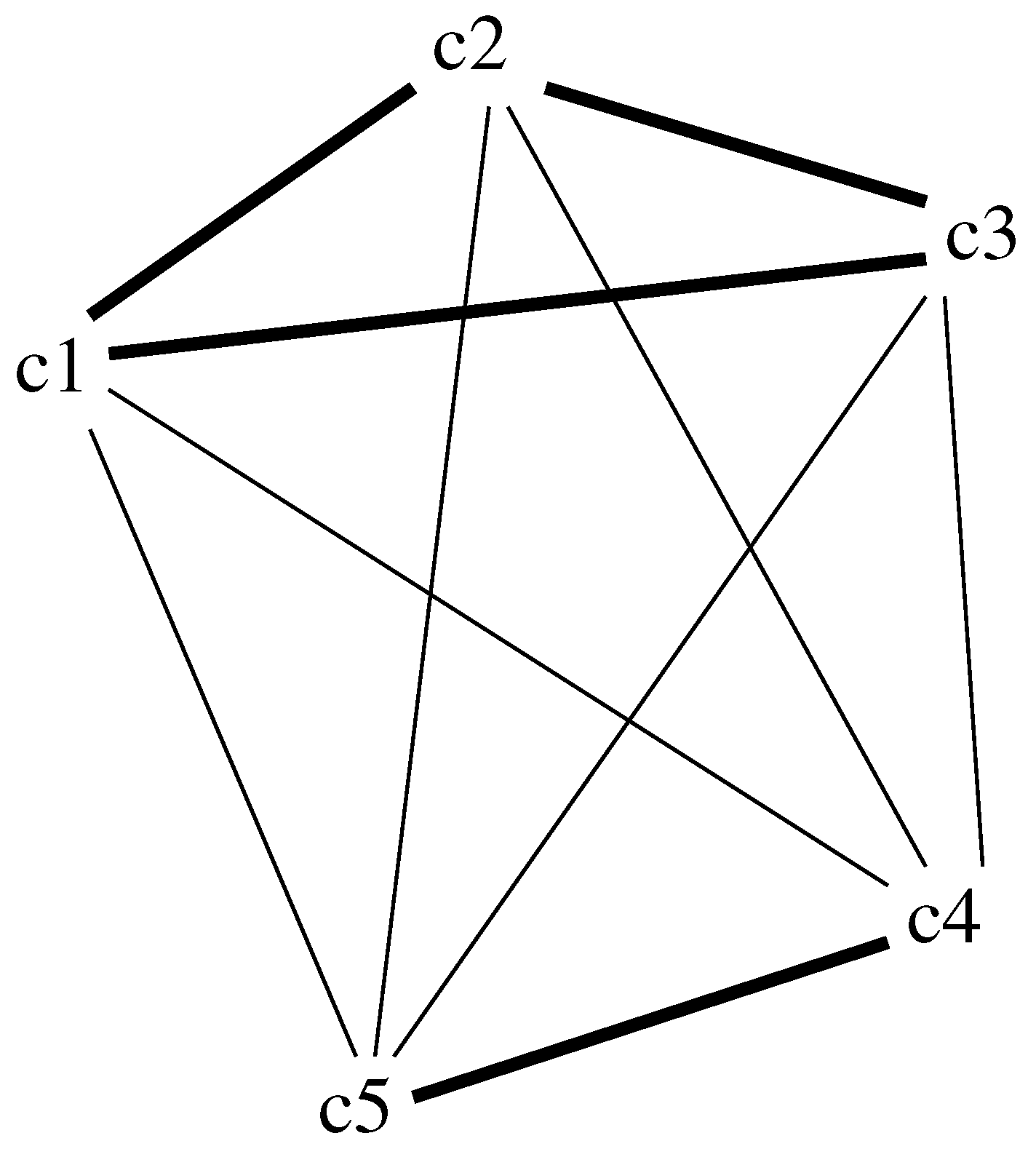
This algorithm can be observed from a graph perspective. The matrix can be seen as a graph (see
Figure 1) that connects some pairs of criteria. Randomness corresponds to selecting a path that traverses nodes in the graph (at most once). All criteria not connected will have a weight of zero (they are seen as redundant to the ones existing).
We first select a criteria (ith criteria). Then, the first loop of the algorithm (Steps 5–6) deals with selecting the remaining criteria with non-zero weights. The second loop (Steps 7–8) will assign the weights of all other criteria to zero.
In the first loop we have that we select in Step 5.1 a new criteria among the ones that are not yet selected (not in ). We select the criteria at random with a probability based on its relevance or eligibility. That is, if the last criterion considered is and if are the criteria pending to be selected at iteration k, we consider a probability distribution where for each criterion its probability of being selected is a function of . For example, we can just use .
Step 5.3 assigns a weight to the new selected criterion . The higher the relevance of the new criterion with respect to all the ones already selected (), the higher the weight.
Using this algorithm, and assuming that the iteration selects , , , , and in this order, we will get their weights equal to , , , , and . That is, , , , , ).
When weights are extracted to be used for the weighted mean, the weights obtained from the algorithm need to be normalized. Therefore, we will have .
We give another example detailing all the steps.
Example 2. We use again the matrix introduced above in Example 1. We will proceed according to the following steps. We use .
When the aggregation operator is the Choquet integral, and the measure is of the family of Sugeno
-measures, we can use the approach proposed in Reference [
19], see also References [
6] (Section 5.3.1) and [
20].
We can prove some properties of the algorithm above.
Proposition 2. Let be the weights obtained from the algorithm above. Then, the following holds.
The weights are the largest importance for any criterion. When the values in the matrix are at most one, all the other weights will be at most α. This follows from Step 5.3 above.
When all criteria are independent, the relative preference matrix is defined with for . This implies that for all i.
Using different criteria as starting points will result into different sets of weights. Differences can also arise because of the random selection of a new criteria in Step 5.1.
The first two properties were given in Reference [
15]. We can illustrate the last property considering three criteria
,
and
where the first two are rather redundant (similar) (
) and the third one is complementary (
). Then, considering the order
we get
and considering the order
we get
. These results are also obtained with other orderings. An average of these weights will result into
which will average the two similar criteria.
We formulate this idea in the following hypothesis.
Note 1. The average of the weights obtained from different paths will result into weights that average redundant criteria.
When the weights are used to build a Sugeno -measure, the following holds which makes the definition consistent with the interpretation of fuzzy measures.
Proposition 3. (See Reference [15] for a proof) Let for all and ; then, the following can be proven: When with n the number of criteria, we have that and the measure is additive. This produces the following measure: for all i.
When , then , and the measure is a plausibility.
When , then , and the measure is a belief.
The first condition shows that when all criteria are independent and , we will obtain an additive fuzzy measure, which means that the fuzzy integral will reduce to the arithmetic mean. This makes the approach consistent, as equally important independent criteria are usually aggregated using the arithmetic mean.
3.4. Measure Determination
When a hierarchical structure is considered we can proceed in a way similar to what has been defined for a matrix.
Step 1. for all
Step 2. Apply the algorithm for a matrix to obtain weights .
Step 3. For each chain in C do
- -
Step 3.1 For each set but lastdo
- *
Step 3.1.1
- *
Step 3.1.2 ifthen
- -
Step 3.2 End for
Step 4. End for
Step 5. for all
Step 6. for all
This definition will construct a fuzzy measure that is normalized (i.e., ) and monotonic (as is positive for all A). Observe that can be seen as the Möbius transform of the measure. This means that (as all are positive) the measure built will be a belief measure.
In Step 3.1.2 we only assign a value to when this is not already assigned. Note that if the relative preference hierarchical structure is consistent, any assignment will just assign the same value. We may consider non consistent structures by means of averaging values (in line with Note 1).
Given a relative preference structure it is easy to define a relative preference hierarchical structure.
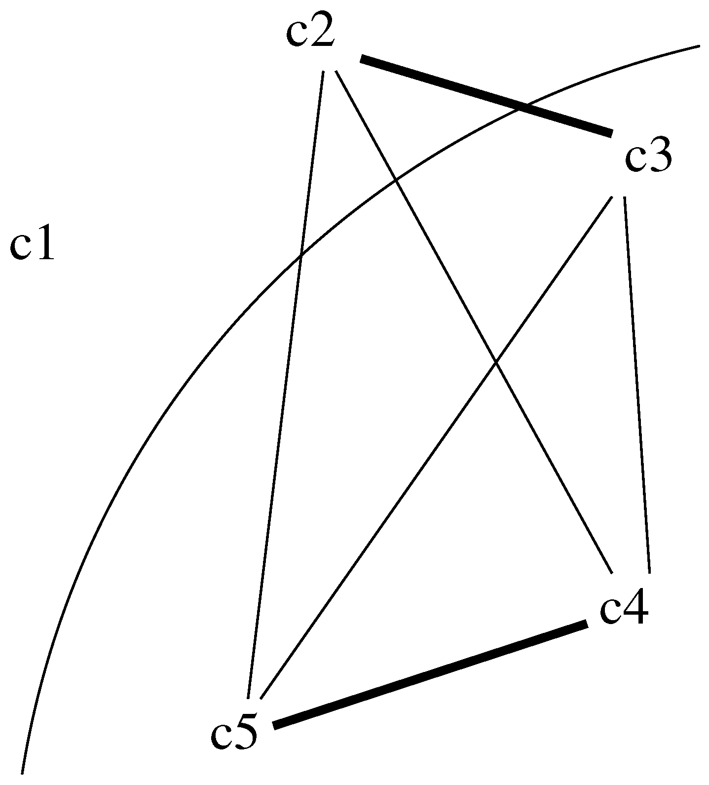
Definition 7. Given a relative preference structure defined by a matrix where corresponds to the pair of criteria and , we define a relative preference hierarchical structure as follows. The set of chains is defined in terms of all possible increasing sets. Then, we use the following function For this definition, Step 3.1.2 means to consider a set
and add an element
e into the set. For illustration consider
and
. We illustrate the definition of
in
Figure 2. In the figure we represent the edges between
and the set
. According to the definition of
d above, we have that
.


