Article

A Mathematical Model of the Transition from Normal Hematopoiesis to the Chronic and Accelerated-Acute Stages in Myeloid Leukemia

by
Lorand Gabriel Parajdi
1,
Radu Precup
1,*,
Eduard Alexandru Bonci
2,3 and
Ciprian Tomuleasa
4
1
Department of Mathematics, Babeş–Bolyai University, 400084 Cluj-Napoca, Romania
2
Department of Oncology, Iuliu Haţieganu University of Medicine and Pharmacy, 400012 Cluj-Napoca, Romania
3
Department of Surgical Oncology, Ion Chiricuţă Clinical Cancer Center, 400015 Cluj-Napoca, Romania
4
Department of Hematology, Ion Chiricuţă Clinical Cancer Center, 400015 Cluj-Napoca, Romania
*
Author to whom correspondence should be addressed.
Mathematics 2020, 8(3), 376; https://doi.org/10.3390/math8030376
Submission received: 20 January 2020 / Revised: 29 February 2020 / Accepted: 3 March 2020 / Published: 8 March 2020
(This article belongs to the Special Issue Mathematical Biology: Modeling, Analysis, and Simulations)

Abstract

:
A mathematical model given by a two-dimensional differential system is introduced in order to understand the transition process from the normal hematopoiesis to the chronic and accelerated-acute stages in chronic myeloid leukemia. A previous model of Dingli and Michor is refined by introducing a new parameter in order to differentiate the bone marrow microenvironment sensitivities of normal and mutant stem cells. In the light of the new parameter, the system now has three distinct equilibria corresponding to the normal hematopoietic state, to the chronic state, and to the accelerated-acute phase of the disease. A characterization of the three hematopoietic states is obtained based on the stability analysis. Numerical simulations are included to illustrate the theoretical results.

1. Introduction

Mathematics can offer qualitative and quantitative tools for a better understanding, prediction, and control of biological processes. Particularly, such tools and models have been given for blood cell production process and hematological disorders. Among the first papers in this direction one can mention the works of Rubinow and Lebowitz [1,2], Mackey and Glass [3], Mackey [4], and Djulbegovic and Svetina [5]. For more recent contributions we refer to Fokas et al. [6], Neiman [7], Andersen and Mackey [8], Colijn and Mackey [9], Adimy et al. [10], Dingli and Michor [11], Kim et al. [12], Cucuianu and Precup [13], Doumic-Jauffret et al. [14], Komarova [15], Stiehl and Marciniak-Czochra [16], MacLean et al. [17,18], Radulescu et al. [19], Bianca et al. [20,21], Ragusa and Russo [22], and to the references therein. For some models concerning stem cell transplantation, we mention the papers of Vincent et al. [23], De Conde et al. [24], Kim et al. [25], Marciniak-Czochra and Stiehl [26], Precup et al. [27,28], Precup [29], and Stiehl et al. [30]. Some reviews that work on mathematical models for cancer, particularly for chronic myeloid leukemia, are the papers of Afenya [31], Michor [32], Foley and Mackey [33], and Clapp and Levy [34].
Hematological stem cells (HSC) from bone marrow are situated at the origin of the process of cell formation. They have the self-renewal capacity and the ability to differentiate and produce various types of blood cells. Perturbations of this complex biological process are at the root of several hematological diseases, such as chronic myeloid leukemia (CML), a malignant disease arising from mutant stem cells affecting the line of myeloid cells and progressing in three phases: chronic (also called indolent) phase, accelerated or transitory phase, and acute or blast phase. The separation of the last two phases being difficult, we shall refer to them as a whole, naming it the accelerated-acute phase.
An analogy can be drawn between the evolution of normal and abnormal stem cell populations and the spread of two species into ecological habitats. Mathematically this evolution is expressed by a differential system involving a number of specific parameters. Such a model for CML, proposed by Dingli and Michor [11], yields to a mathematical characterization of two hematological states: normal state and leukemic state, without being able to make distinction between the chronic and accelerated-acute phases of the disease. Further analysis of the model and its extensions for bone marrow transplantation have been undertaken by Precup and co-workers (Cucuianu and Precup [13], Precup et al. [27,28], and Precup [29]).
In this paper we propose a refined version of the Dingli–Michor differential system that allows us to make the distinction between the following three hematopoietic states related to chronic myeloid leukemia: normal hematopoietic state, chronic leukemic state, and accelerated-acute state. We assume normal hematopoietic state as a biological state in which the population of one or more mutant hematopoietic stem cells (mHSC) tends to zero due to random events that lead to the extinction of mutant cells, a fact demonstrated experimentally in stem cell lineages (see Jilkine and Gutenkunst [35], Driessens et al. [36], Klein et al. [37], Lopez-Garcia et al. [38], and Snippert et al. [39]). We accomplish our purpose by operating with distinct sensitivity parameters for normal and abnormal cells, instead of a single common parameter, like the one that was used in the original model. Our modeling choice is biologically justified by the asymmetry of mutual influences and interactions between normal and leukemic cells (Gou et al. [40]). The new model, also expressed by a two-dimensional differential system, has three nontrivial steady states, and their stability analysis shows that only one of them is asymptotically stable depending on the value of a cumulative parameter D that incorporates the growth rate, the cell death rate, and the sensitivity rate of the abnormal cells, and represents the equilibrium amount of abnormal cells. Values of D under some threshold correspond to the normal hematological state; values of D lying in some interval characterize the chronic phase, while larger values of D stay for the accelerated-acute phase (see Figure 1 below). In this way, from a mathematical point of view, the transition from one hematological state to another occurs as the result of a change of the basic leukemic cell parameters accumulated by D . The transition is progressive as the disease gets worse, and regressive as a result of treatment. For the last case, our analysis could be a guide to the improvement of therapeutic agents and strategies, as suggested in Precup et al. [41].
The paper is structured as follows: In Section 2, we consider the new model and we carry out its mathematical analysis. Based on this model, the normal hematopoietic state, and the chronic and accelerated-acute phases of CML are mathematically characterized in terms of parameter D . In Section 3, we provide some numerical simulations of the model. Next, in Section 4, the model is upgraded by six additional equations so that, as in Michor et al. [42] and Dingli and Michor [11], it becomes able to describe the cell evolution on four levels: primitive stem cells, progenitors, differentiated cells and terminally differentiated cells. The numerical simulations show the parallelism between the dynamics of primitive stem cells and that of the succeeding lines, which allows the analysis to be performed at any level, particularly for terminally differentiated cells for which laboratory data can be obtained easier. Finally, in Section 5, some medical remarks and conclusions are included. We conclude this introductory section with medical background addressed to those readers that would like to have more biological and medical information about hematopoiesis, malignant disorders, and related literature.

Medical Background

Hematopoiesis is the process of blood cell formation. The process starts in the intrauterine life in the mesoderm of the yolk sac and continues in the liver and the spleen during the second and seventh month. It then takes place at the level of the bone marrow, where it carries on after birth. During childhood, hematopoiesis takes place in almost all bones, gradually being replaced with growth by fat tissue. In adults, hematopoiesis occurs only in the pelvis, vertebrae, sternum (Howard et al. [43] and Young [44]), ribs, skull, proximal humerus, and femur epiphysis (Kaushansky et al. [45]).
Hematopoiesis and the differentiation process into various blood cell types can be viewed as an evolutionary tree that grows from one single hematopoietic stem cell (HSC). A HSC can have one of the following functions: it can renew itself; it can generate two other HSCs; or it can lose the ability of self-renewal and begin the maturation and differentiation pathway resulting two progenitor cells; or finally, it can give birth to a HSC and a progenitor cell. Progenitor cells are capable of initiating the differentiation towards one of the pathways that lead to the formations of various types of blood cells: common lymphoid progenitor (CLP) that will differentiate and maturate into B or T-lymphocytes, and the common myeloid progenitor (CMP) that will differentiate and maturate into leukocytes (white blood cells), erythrocytes (red blood cells), and platelets (Young [44] and Kaushansky et al. [45]). According to recent studies, there is growing evidence that hematopoietic stem cells produce a common myeloid progenitor and a common myelo-lymphoid progenitor (CMLP) that in their turn produce a bipotential myeloid T progenitor and a myeloid B progenitor (Kawamoto et al. [46]).
Although HSCs have the unique properties of leading to the formation of blood cells (self-renewal capacity and the ability to differentiate and produce different blood cells), they are dependent on several other factors: the environment that enables cell-to-cell and cell-to-matrix interaction (micromedia, niche), cytokines (growth, proliferation, differentiation and maturation factors) and humoral feedback from peripheral target tissue (Howard et al. [43], Young [44], Kaushansky et al. [45], Abkowitz [47], Cucuianu and Precup [13]). These unique properties are dependent upon two major groups of control factors: intrinsic cell factors (DNA alterations) and extrinsic cell factors (microenvironment factors, humoral feedback, cytokines) (Ramalingam et al. [48] and Zon [49]).
Even though mammals, humans included, have a stock of only 2 × 10 4 HSCs (Abkowitz [47]), they can give birth and release into the blood stream approximately 2.5 billion erythrocytes/kg/day, 2.5 billion platelets/kg/day and 1 billion granulocytes/kg/day.
Leukemias are an heterogeneous group of malignant disorders, also known as cancer, arising from one mutant hematopoietic stem cell (mHSC) (Howard et al. [43], Jilkine and Gutenkunst [35] Driessens et al. [36], Klein et al. [37], Lopez-Garcia et al. [38], and Snippert et al. [39]). In this study, we analyze the dynamics of HSCs and mHSCs by assuming that at least one mHSC can be found in the human body. Therefore, the complex biological processes on which the hematopoiesis is based are not completely involved.
There are four main types of leukemia (based on their progression-chronic or acute, and on the type of the affected cell-myeloid or lymphoid) (Neiman [7]). Although current guidelines include a more comprehensive and detailed classification of leukemias (with types and subtypes of cells, mutations acquired, etc.), they do not make the subject of the current study, nor do they bring useful information to our mathematical model (Arber et al. [50]).
The mHSCs have an abnormal process of differentiation and particular characteristics compared to HSCs, due to their acquired genetic and epigenetic abnormalities: increased proliferation/growth advantage; lower sensitivity to apoptosis and to the environment; poor differentiation; squeezing out of normal HSCs from bone marrow (Roeder and d’Inverno [51]). All these can lead to a wide range of clinical results with major impacts on patients’ health.
Chronic Myeloid Leukemia (CML) is an acquired myeloproliferative disorder (Howard et al. [43] and Neiman [7]). The CML is probably the first recognized leukemia, dating back to the 1840s (Young [44]).
CML represents 15% of all types of leukemia, annually occurring in 2 out of every 100,000 men and 1.1 out of every 100,000 women (Hemminki and Jiang [52]). Most frequently, the diagnosis is established during routine blood tests, occurring more frequently after the fifth decade of life (Howard et al. [43]). The signs and symptoms may include anemia, splenomegaly, weight loss, and dyspnea on exertion. Among the risk factors, ionizing radiation was observed to have a role in developing CML (Young [44]).
The hallmark of CML is the Philadelphia chromosome (Ph). Ph is characterized by a mutation in the normal hematopoietic stem cell population (Howard et al. [43]), generated by one abnormal stem cell, with the t(9;22)(q34;q11) (Young [44]) mutation, a reciprocal translocation of the ABL gene from chromosome 9 to chromosome 22, next to the BCR gene. This newborn BCR-ABL gene codes a fusion protein with tyrosine kinase activity, which apparently influences whether the cell lives or dies, and proliferates or not.
This type of leukemia typically undergoes three phases: chronic (also called indolent) phase, accelerated or transitory phase, and acute/blast phase (Abkowitz [47] and Arber et al. [50]). Due to the difficulty of separating the accelerated phase from the blast phase, we will refer to them as a whole, naming it the accelerated-acute phase. Most cases are diagnosed during the chronic phase and rarely during one of the other two phases. Once the mutation has occurred in one HSC, it starts a series of divisions, followed by differentiation and maturation that no longer obey the feedback and control mechanisms that apply to healthy HSCs. Therefore, the mutant cells divide at a quicker rate, producing a large number of thrombocytes and leukocytes, resulting in a population of cells where mHSCs are dominant.
At a certain point of CML, the occurrence of other events (most probably the acquisition of other genetic mutations) leads to an instability of the mHSC population, which consequently leads to an accelerated-acute phase, resulting in an exponential increase of the number of immature stem cells. Cells multiply in a more accelerated manner and do not undergo differentiation, resulting in a blast phase, similar to various types of acute leukemia (myeloid—70%, lymphoid—20%, and mixt type—10%) in terms of symptoms and clinical findings (Young [44], Abkowitz [47], and Neiman [7]). After reaching the accelerated phase or the blast phase, patients have a median survival of 4.8 years or 6 months, respectively (Kantarjian et al. [53]).
In terms of treatment, even though tyrosinkinase inhibitors are effective in 70%–80% of cases of CML, stem cell transplantation (SCT) seems to be the only curative treatment, involving, nevertheless, a high mortality rate due to complications (Howard et al. [43] and Thomas [54]).

2. The Mathematical Model

In this section, we give the mathematical model, we obtain the associated steady states, and we investigate their stability. Based on this analysis, we characterize the normal hematopoietic state, and the chronic and accelerated-acute stages in CML.

2.1. The Normal-Leukemic Dynamic System
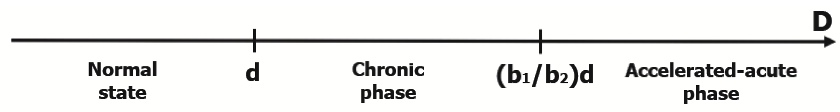
The mathematical modeling of the time evolution of a population p of any nature begins in a first approximation (assuming no constraints exist) with the Malthusian equation
d p d t = a p c p ,
where p = p t is the population size at time t , and a and c are the growth and death (per capita) rates, respectively. Assuming that the growth rate is bigger than the death rate, the population will increase exponentially according to the law
p t = p ( 0 ) exp a c t ,
which is non-realistic in the long run, particularly for limited biological populations. Thus, a more realistic approach is to consider that the growth (and/or death) rate will change during evolution by a self-limiting mechanism or exterior influences. For instance, the growth rate of a self-limiting population can be a / 1 + b p depending on the population size itself. Here, b is a proportionality factor that shows how sensitive that population is with respect to its own size. This shows that the growth rate decreases as the population size p increases. In addition, the influence over p of a competitive population q = q t can be simulated in the model by a growth rate of the form a / 1 + b 1 p + b 2 q , where the ratio b 2 / b 1 shows how strong the diminishing effect due to population q is, compared to that of self-limitation.
Applied to the normal and abnormal stem cell populations denoted by x and z , the above modeling choice leads to the following differential system
d x d t = a 1 + β 1 x + β 2 z x c x d z d t = A 1 + γ 1 x + γ 2 z z C z .
Here, since abnormal cells have a stronger diminishing effect on the growth rate of normal cells than on their own growth rate, it is natural to assume that
β 2 > γ 2 .
Additionally, the almost negligible effect of normal cells over the growth rate of population z (i.e., γ 1 is much smaller than β 1 ) justifies the inequality
γ 2 γ 1 > β 2 β 1 .
For the mathematical analysis of most models, it is often convenient that the number of parameters is reduced as much as possible. Thus, in our case, we can reduce the number of parameters β 1 , β 2 , γ 1 , γ 2 to three by making the change of variable (equivalently, by rescaling the abnormal cell population)
y = γ 2 γ 1 z .
Substituting in (1) yields the system
d x d t = a 1 + b 1 x + b 2 y x c x
d y d t = A 1 + B ( x + y ) y C y .
where
b 1 = β 1 , b 2 = β 2 γ 1 γ 2 , B = γ 1 .
Then (3) yields b 1 > b 2 , which shows the different contributions of the normal and abnormal stem cells to the diminution of the nonrestrictive growth rate of the normal cell population, while (2) guarantees that b 2 > B , reflecting the eventual advantage of the abnormal cells of being less sensitive to the bone marrow microenvironment.
The system (4)–(5) is our basic model for normal-leukemic cell evolution. Here, the model parameters a and A are the nonrestrictive growth rates (due to self-renewal) of normal and abnormal stem cells, respectively; b 1 , b 2 and B are the bone marrow microenvironment sensitivities; while c and C stand for their cell death rates (due to differentiation, apoptosis, and other elimination mechanisms) (see Alenzi et al. [55], Cisneros et al. [56], Domen [57], Riether et al. [58], Vivier et al. [59]). The terms
1 1 + b 1 x + b 2 y and 1 1 + B ( x + y )
quantify the impact of the induced crowding in the bone marrow microenvironment, introduce competition between normal and abnormal cells, and guarantee homeostasis at the level of cell population. We assume that for both cell populations, the growth rate is greater than the death rate, that is,
a > c and A > C .
Note that an alternative model for normal-abnormal dynamics can be found in Neiman [7], where the role of the parameter b 1 / b 2 is given by a parameter denoted by g and assumed greater than or equal to one.
The case b 1 = b 2 was considered by Dingli and Michor [11] and Cucuianu and Precup [13]. In this case there are only two non-zero steady states, ( d , 0 ) and ( 0 , D ) , where d and D represent the homeostatic amounts of normal and abnormal stem cells, and they are given by
d = 1 b 1 a c 1 a n d D = 1 B A C 1 .
In this paper we assume that b 1 > b 2 . As we shall see, in this case, besides the non-zero steady states ( d , 0 ) and ( 0 , D ) , a steady state ( x * , y * ) could also exist with both positive components, i.e., x * > 0 and y * > 0 . This makes the new model able to differentiate between chronic and accelerated-acute phases in CML.
We continue to analyze the system (4)–(5).
(a) Monotonicity of the solutions. The function x ( t ) increases during the time intervals where d x / d t > 0 , i.e., a / ( 1 + b 1 x t + b 2 y t ) c > 0 , or equivalently x ( t ) + ( b 2 / b 1 ) y ( t ) < d . Hence,
x ( t ) increases as long as x ( t ) + b 2 b 1 y ( t ) < d , x ( t ) decreases as long as x ( t ) + b 2 b 1 y ( t ) > d .
From a biological point of view, the increasing or decreasing of the normal cell population occurs on those intervals of time where the weighted total of cells remains under or upper the normal homeostatic level, respectively.
Similarly,
y ( t ) increases as long as x ( t ) + y ( t ) < D , y ( t ) decreases as long as x ( t ) + y ( t ) > D .
(b) Steady states. A steady state (or an equilibrium) is a constant solution, i.e., a solution for which d x / d t = d y / d t = 0 . Hence, the steady states are obtained by solving the algebraic system
a 1 + b 1 x + b 2 y x c x = 0
A 1 + B ( x + y ) y C y = 0 .
The solutions of the system (7a)–(7b) are the pairs
( 0 , 0 ) , ( d , 0 ) , ( 0 , D ) and ( x * , y * ) ,
where d , D are given by (6),
x * = b 2 c ( A C ) B C ( a c ) B C c ( b 1 b 2 )
and
y * = b 1 c ( A C ) B C ( a c ) B C c ( b 1 b 2 ) .
Direct calculation leads to
x * = b 1 b 1 b 2 d b 2 b 1 b 2 D , y * = b 1 b 1 b 2 D d .
It is easy to see that under the assumption that b 1 > b 2 , both numbers x * and y * are positive (acceptable values from a biological point of view) if and only if
d < D < b 1 b 2 d .
Therefore, in addition to the non-zero steady states d , 0 and 0 , D , a positive steady state x * , y * appears, contrary to the case where b 1 = b 2 .
(c) Stability. We study the stability of the steady states of the system (4)–(5) using the standard first approximation method (for details see Kaplan and Glass [60], Coddington and Levinson [61] and Jones et al. [62]). According to this method, an equilibrium ( α , β ) is asymptotically stable if the Jacobian matrix J ( α , β ) is a Hurwitz matrix, i.e., Re λ < 0 for all its characteristic roots λ , and is unstable if Re λ > 0 for at least one of its characteristic roots.
It should be emphasized that the local stability that we analyze below coincides with the global stability of the corresponding equilibria. This guarantees that the predictions are robust to uncertainties in the initial cell counts.
Note that the steady state ( 0 , 0 ) is unstable as can be shown based on the assumptions a > c and A > C .
For the steady state ( d , 0 ) , the eigenvalues of the Jacobian matrix J ( d , 0 ) are
λ 1 = c ( a c ) a , λ 2 = b 1 c ( A C ) B C ( a c ) b 1 c + B ( a c ) .
Obviously λ 1 < 0 . Thus, the steady state ( d , 0 ) is asymptotically stable if and only if λ 2 < 0 , or equivalently, if D < d . On the contrary, if D > d , then the equilibrium ( d , 0 ) is unstable.
The eigenvalues of the Jacobian matrix J ( 0 , D ) associated to the equilibrium 0 , D are
λ 1 = b 2 c ( A C ) B C ( a c ) b 2 ( A C ) + B C , λ 2 = C ( A C ) A .
Here λ 2 < 0 , and so the steady state ( 0 , D ) is asymptotically stable if and only if λ 1 < 0 . This happens if D > ( b 1 / b 2 ) d . Contrarily, if D < ( b 1 / b 2 ) d , then the steady state ( 0 , D ) is unstable.
In the chronic case d < D < ( b 1 / b 2 ) d , by direct computation, we easily find the following representation of the Jacobian matrix J ( x * , y * )
J x * , y * = b 1 c 2 a x * b 2 c 2 a x * B C 2 A y * B C 2 A y *
whose characteristic polynomial is
λ 2 λ tr J x * , y * + det J x * , y * ,
where
tr J x * , y * = b 1 c 2 a x * B C 2 A y * , det J x * , y * = B c 2 C 2 a A b 1 b 2 x * y * .
Obviously tr J x * , y * < 0 and det J x * , y * > 0 . These imply that J x * , y * is a Hurwitz matrix. Hence the equilibrium x * , y * is asymptotically stable.
The above discussion shows a qualitative change of the system’s behavior, i.e., a change of stable equilibrium where the parameter D varies. The values of this parameter at which the stable equilibrium changes (called bifurcation points) are D = d and D = ( b 1 / b 2 ) d . We can summarize the bifurcation analysis of our system as follows (see Figure 1):
  • If D < d , then the steady state ( d , 0 ) is asymptotically stable, and the steady state ( 0 , D ) is unstable.
  • If d < D < ( b 1 / b 2 ) d , then the steady state ( x * , y * ) is positive and asymptotically stable, and the steady states ( d , 0 ) and ( 0 , D ) are unstable.
  • If D > ( b 1 / b 2 ) d , then the steady state ( 0 , D ) is asymptotically stable, and the steady state ( d , 0 ) is unstable.
From a biological point of view, as long as normal cells have an advantage over abnormal cells d > D , the healthy state may not present any perceptible changes. A balance between normal and abnormal cells will exist as long as abnormal cells have a not too large advantage over normal cells d < D < b 1 / b 2 d , and the balance is disturbed, leading to an accelerated-acute phase of the disease, once the advantage of leukemic cells becomes significant D > b 1 / b 2 d (see Stine and Matunis [63]).

2.2. The Mathematical–Biological Interpretation

In view of the above discussion, we can claim that the relationship D < d characterizes the normal hematopoiesis; the relationship d < D < ( b 1 / b 2 ) d stands for the chronic phase of leukemia; meanwhile, the inequality D > ( b 1 / b 2 ) d characterizes the accelerated-acute phase of the disease. Indeed (see Figure 2), in the case where D < d , the normal cell population x t approaches the equilibrium abundance d (normal homeostatic state) while the abnormal cell population y t tends in time to zero; in the case where d < D < ( b 1 / b 2 ) d , the cell populations x t and y t approach their equilibrium abundances x * and y * , respectively; finally, if D > ( b 1 / b 2 ) d , then the leukemic cell population becomes dominant approaching its equilibrium abundance D (leukemic homeostatic state) and leads to the elimination of the normal cells, i.e., x t tends to zero.
Finally, a condition like D = d or D = ( b 1 / b 2 ) d is physiologically very unstable, since small variations of the kinetic parameters can switch the normal state into the chronic leukemic state and vice-versa, if D = d , and can switch the chronic state into the accelerated-acute phase and vice-versa, if D = ( b 1 / b 2 ) d . Additionally, from a medical point of view, the situations D = d and D = ( b 1 / b 2 ) d are practically undetectable.
In terms of the system’s biological growth parameters, the hematological states are characterized as follows:
1 B A C 1 < 1 b 1 a c 1 normal state ; 1 b 1 a c 1 < 1 B A C 1 < 1 b 2 a c 1 chronic phase ; 1 b 2 a c 1 < 1 B A C 1 accelerated - acute phase .
A diagram of the transition from normal hematopoiesis to chronic and accelerated-acute stages in CML is presented in Figure 1. Notice that the length of the interval d , b 1 / b 2 d that corresponds to the chronic phase is b 1 / b 2 1 d and depends on the ratio b 1 / b 2 . The bigger the ratio b 1 / b 2 is, the larger the interval in which a patient’s parameter D can lay in chronic phase. Notice that the patient-related parameter b 1 / b 2 gives the ratio of contributions of the normal and abnormal stem cells to the diminution of the nonrestrictive growth rate of the normal cell population, aiming to restore homeostasis.
According to our model, values of parameter D close to d correspond to early stages of the disease, while values of D close to b 1 / b 2 d indicate advanced stages of the disease moving towards the accelerated-acute phase.

3. Numerical Simulation of the Model

Further on, we illustrate the theoretical results on the system (4)–(5) by numerical simulations using the Maple package.

3.1. Parameter Estimations

The parameters employed by our model depend on a large number of biophysical and biochemical mechanisms. The latter make the exact estimation of these parameters almost impossible. Instead, one may expect that from any estimation procedure with confidence intervals, parameters are obtained. For a qualitative analysis such as ours, parameter estimation is not essential, and as already seen, relationships between parameters are enough. Parameter estimation becomes essential when the model is applied for real-time predictions and individual patients.
According to the paper of Dingli and Michor [11], the number of the stem cells in a healthy adult body is approximately d = 2 × 10 4 (normal homeostatic state), and the growth and death rates of normal stem cells could be taken a = 0.005 and c = 0.002 . However, recent studies have shown different growth rates of HSC. One study concluded that HSCs divide on average every 40 weeks, with a range from 25 to 50 weeks (see Catlin et al. [64]). Others even suggested the existence of two types of HSCs with different replication rates (dormant HSCs divide about every 145 days, active HSCs divide about every 36 days) (see Wilson et al. [65]). Regarding the life span of HSC, recent studies have suggested a death rate ranging from 10 to 60 months (see Sieburg et al. [66] and Sieburg et al. [67]). The factor b 1 / b 2 allows for the possibility that the abnormal stem cells are less sensitive to the bone marrow microenvironment than the normal cells. The parameter b 1 that stands for the bone marrow microenvironment sensitivity of the normal stem cells can be estimated from the expression of d, namely, b 1 = a / c 1 / d = 0.75 × 10 4 .
Parameters A , B , C and b 2 vary from patient to patient, and so do parameter D and the length of the chronicity interval d , b 1 / b 2 d . For our numerical simulations we choose value 2 for b 1 / b 2 and we then have b 2 0.38 × 10 4 . Additionally, as in Dingli and Michor [11], we assume that the value of parameter B is approximately half of b 2 ; hence, B 0.19 × 10 4 . As regards the parameters A and C , several values are considered in our simulations such that all the previous relationships between the model parameters hold.

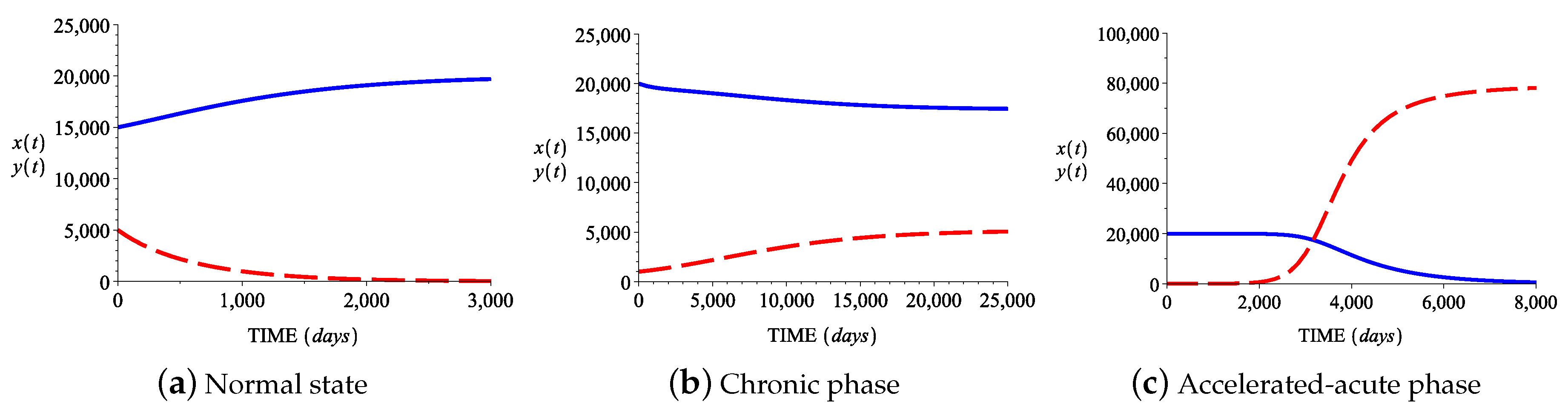
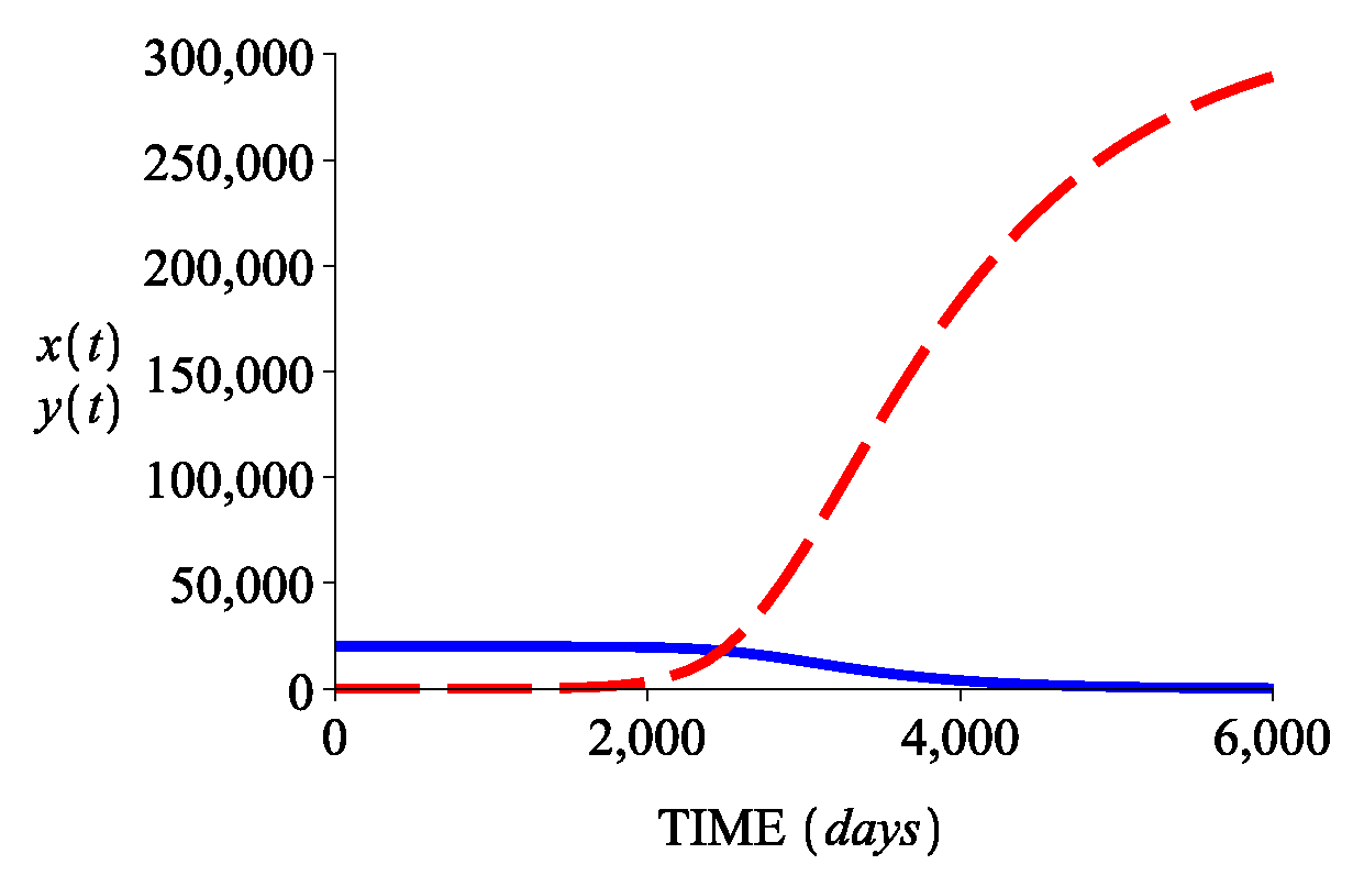
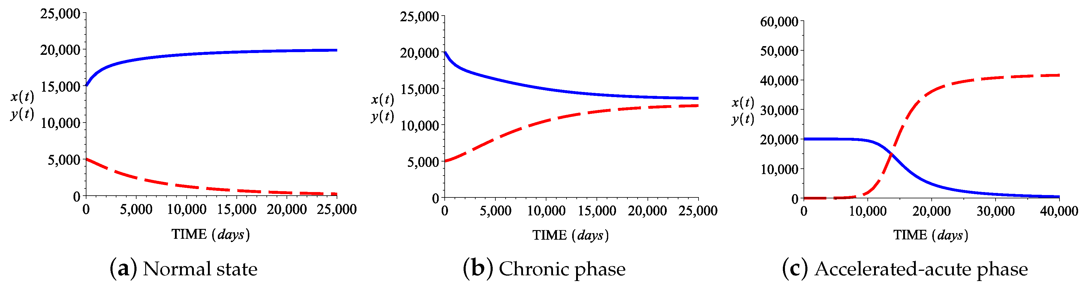
3.2. Numerical Simulations

We simulate numerically system (4)–(5) in order to investigate the behavior of normal and abnormal stem cell populations in each of the cases: D < d (normal state); d < D < ( b 1 / b 2 ) d (chronic state); and ( b 1 / b 2 ) d < D (accelerated-acute state). The graphs of x ( t ) (blue solid line) and y ( t ) (red broken line) for a time interval 0 t T , are represented for different sets of values of the model parameters: a , b 1 , b 2 , c , A , B , C ; initial values x ( 0 ) , y ( 0 ) ; and length T of the time interval.
We shall restrict our simulations to the situations presented in Table 1. In all of the cases we assume that the abnormal stem cells are less sensitive to environmental crowding than the normal stem cells, that is, b 1 > b 2 > B .
Case I: In this case the growth and death rates of normal stem cells are smaller than the growth and death rates of abnormal stem cells. Figure 3a shows the behavior in time ( T = 3000 days) of the two cell populations for the parameter values provided in the first line in Table 2, values that correspond to the normal hematopoietic state ( D < d ). The normal stem cell population x ( t ) (blue solid line) tends to the value d while the abnormal stem cell population y ( t ) (red broken line) tends towards 0. Biologically, this mutant/abnormal cell extinction, due to random events, has been explained and demonstrated in several studies using stem cell lineages (see Jilkine and Gutenkunst [35], Driessens et al. [36], Klein et al. [37], Lopez-Garcia et al. [38], and Snippert et al. [39]). Figure 3b shows the behavior in time ( T = 25,000 days) of the two cell populations for the parameter values from the second line of Table 2, values that correspond to the chronic state d < D < ( b 1 / b 2 ) d . The normal and leukemic stem cell populations x ( t ) , y ( t ) tend toward x * and y * , respectively. Figure 3c shows the behavior in time ( T = 8000 days) of the two cell populations for the corresponding parameter values from Table 2, values that lead to the accelerated-acute state D > ( b 1 / b 2 ) d . The normal stem cell population x ( t ) tends towards 0 , while the leukemic stem cell population y ( t ) tends to the value D .
Case II: Here the growth rate of normal stem cells is smaller than the growth rate of abnormal stem cells, and the death rate of normal stem cells is greater than the death rate of abnormal stem cells. Then A / C > a / c , and since 1 / B > 1 / b 2 , we immediately see that 1 / B A / C 1 > 1 / b 2 a / c 1 , or equivalently D > b 1 / b 2 d . Hence, in this case only the accelerated acute state is possible. Figure 4 shows the behavior in time ( T = 6000 days) of the two cell populations for the corresponding parameter values from Table 2. The normal stem cell population x ( t ) tends towards 0 , while the leukemic stem cell population y ( t ) tends to the value D .
Case III: In this case, the growth rate of normal stem cells is greater than the growth rate of abnormal stem cells, and the death rate of normal stem cells is smaller than the death rate of abnormal stem cells. Figure 5a shows the behavior in time ( T = 25,000 days) of the two cell populations for the corresponding parameter values from Table 2, values that correspond to the normal hematopoietic state D < d . The normal stem cell population x ( t ) becomes arbitrarily close to the value d , while the abnormal stem cell population y ( t ) tends towards 0 . Figure 5b shows the behavior in time ( T = 25,000 days) of the two cell populations for the corresponding parameter values from Table 2, values that correspond to the chronic state d < D < ( b 1 / b 2 ) d . The normal and leukemic stem cell populations x ( t ) , y ( t ) tend toward x * and y * , respectively. Figure 5c shows the behavior in time ( T = 40,000 days) of the two cell populations for the corresponding parameter values from Table 2, values that lead to the accelerated acute state D > ( b 1 / b 2 ) d . The normal stem cell population x ( t ) tends towards 0 , while the leukemic stem cell population y ( t ) tends to the value D .
Case IV: In this case, the growth rate of normal stem cells is greater than the growth rate of abnormal stem cells, and the death rate of normal stem cells is greater than the death rate of abnormal stem cells. Figure 6a shows the behavior in time ( T = 25,000 days) of the two cell populations for the corresponding parameter values from Table 2, values that correspond to the normal hematopoietic state D < d . Normal stem cell population x ( t ) tends to the value d , and abnormal stem cell population y ( t ) approaches 0 . Figure 6b shows the behavior in time ( T = 25,000 days) of the two cell populations for the corresponding parameter values from Table 2, values that correspond to the chronic state d < D < ( b 1 / b 2 ) d . The normal and leukemic stem cell populations x ( t ) , y ( t ) tend toward x * and y * , respectively. Figure 6c shows the behavior in time ( T = 25,000 days) of the two cell populations for the corresponding parameter values from Table 2, values that lead to the accelerated-acute state D > ( b 1 / b 2 ) d . The normal stem cell population x ( t ) approaches 0 , while the leukemic stem cell population y ( t ) tends to the value D .

4. The Model Extended to Terminally Differentiated Cells

Working at the level of primitive stem cells, there is not an ordinary method to determine the sizes of cell populations. Therefore, it would be useful to have a reflection of the primitive stem cell evolution at the level of terminally differentiated cells, since the latter can be easily estimated by current blood tests.
The idea appears in Michor et al. [42], and when applied to our model yields the extended system
d x 1 d t = a 1 1 + b 1 x 1 + b 2 y 1 x 1 c 1 x 1 ( NSC ) d y 1 d t = A 1 1 + B ( x 1 + y 1 ) y 1 C 1 y 1 ( ASC ) d x 2 d t = a 2 x 1 c 2 x 2 ( NPC ) d y 2 d t = A 2 y 1 C 2 y 2 ( APC ) d x 3 d t = a 3 x 2 c 3 x 3 ( NDC ) d y 3 d t = A 3 y 2 C 3 y 3 ( ADC ) d x 4 d t = a 4 x 3 c 4 x 4 ( NTC ) d y 4 d t = A 4 y 3 C 4 y 4 ( ATC ) .
Here, x 2 t , y 2 t stand for the normal (N) and abnormal (A) progenitor cell (PC) populations; x 3 t , y 3 t stand for the normal and abnormal differentiated cell (DC) populations; and x 4 t , y 4 t stand for the normal and abnormal terminally differentiated cell (TC) populations, respectively.
Notice the different form of the additional six equations associated to the succeeding cell compartments. It is the balance expression of the transfer from one compartment to the next; namely, it states that the rate of change of cell population equals the amount of new cells produced by the anterior compartment minus the amount of cells that leave (by differentiation or apoptosis) that compartment. Thus, the new parameters a 2 , A 2 are the rates at which normal and abnormal progenitor cells are produced from normal and abnormal stem cells; a 3 , A 3 are the rates at which normal and abnormal differentiated cells are produced from normal and abnormal progenitor cells; a 4 , A 4 are the rates at which normal and abnormal terminally differentiated cells are produced from normal and abnormal differentiated cells; and c 2 , c 3 , c 4 , C 2 , C 3 , C 4 are the death rates of normal and abnormal progenitors, and differentiated and terminally differentiated cells.
In the equilibrium state, we assume that in a healthy adult body the number of stem cells is d = x 1 * = 2 × 10 5 , the number of progenitor cells is x 2 * = 1 × 10 8 , the number of differentiated cells is x 3 * = 1 × 10 10 , and the number of terminally differentiated cells is x 4 * = 1 × 10 12 (see Michor et al. [42]). Consequently, in the equilibrium state, we have for progenitor cells a 2 x 1 * c 2 x 2 * = 0 , whence a 2 / c 2 = x 2 * / x 1 * = 5 × 10 2 , for differentiated cells a 3 x 2 * c 3 x 3 * = 0 , whence a 3 / c 3 = x 3 * / x 2 * = 1 × 10 2 , and for terminally differentiated cells a 4 x 3 * c 4 x 4 * = 0 ; hence a 4 / c 4 = x 4 * / x 3 * = 1 × 10 2 . Therefore, if c 2 = 0.008 , c 3 = 0.05 and c 4 = 1 (see Michor et al. [42]), then a 2 = 4 , a 3 = 5 , and a 4 = 100 .
Note that if
( x 1 E , y 1 E )
is any equilibrium (E) of the initial system (4)–(5), then
( x 1 E , y 1 E , a 2 x 1 E / c 2 , A 2 y 1 E / C 2 , a 2 a 3 x 1 E / c 2 c 3 , A 2 A 3 y 1 E / C 2 C 3 , a 2 a 3 a 4 x 1 E / c 2 c 3 c 4 , A 2 A 3 A 4 y 1 E / C 2 C 3 C 4 )
is an equilibrium of the extended system, and the two equilibria have the same stability property. Therefore, working at the level of primitive stem cells is equivalent to working at the level of any one of the succeeding classes of cells. Thus, if by blood tests one estimates the steady state ration x 4 E / y 4 E between healthy and unhealthy terminally differentiated cells as being equal to λ , then we can immediately calculate the analogue steady state ratios of differentiated, progenitor, and stem cells, as follows:
x 3 E y 3 E = λ A 4 c 4 a 4 C 4 , x 2 E y 2 E = λ A 3 A 4 c 3 c 4 a 3 a 4 C 3 C 4 , x 1 E y 1 E = λ A 2 A 3 A 4 c 2 c 3 c 4 a 2 a 3 a 4 C 2 C 3 C 4 .
Figure 7a–d show that there is indeed a parallelism between the behaviors of normal and abnormal cell populations in all four cell compartments.

5. Discussion and Conclusions

By resuming and adding a new parameter to the system created by Dingli and Michor, the present study tried to bring the model and the numerical simulations one step closer to the complex reality of leukemic stem cell evolution, while also maintaining the model simple enough to draw conclusions.
We were able to analyze elements and characteristics of both normal and mutant stem cells, unproven or unnoticed on the original model, but hopefully of some use for the upcoming research and mathematical modeling of leukemic pathology.
By analyzing the numerical simulation for the first case, in which leukemic stem cells had a rate of multiplication higher than that of normal stem cells (in our case two times higher), we observed that the evolution of leukemic pathology was dependent on the ratio given by death rates of the two types of stem cells lines. Therefore, at a mHSC death rate four times higher than that of normal HSC, the disease progressed and led to the disappearance of mHSCs, while in case of a lower death rate of the leukemic stem cells ranging between 4 × c and 3 × c , the disease evolved towards a stabilization of the two stem cell lines; that is, to the chronic phase of CML. Finally, the disease evolution shifted towards the accelerated-acute phase when the mHSC death rate decreased below 3 × c , a situation clinically similar to acute myeloid leukemia (AML). The analysis of the second case reveals to us a very logical conclusion. The leukemic stem cells, having all the advantages (proliferation rate higher than normal stem cells, death rate lower than normal stem cells, and lower sensitivity towards the microenvironment) apparently leads us to only one possible case, that of the accelerated-acute phase of CML. This allowed us to confirm our previously mentioned conclusion, which stated that the disease evolved towards the specific course of the accelerated-acute phase of chronic myeloid leukemia in the absence of a death rate of mHSC several times higher than the death rate of normal stem cells. In terms of medical treatment, this case appears to underline the importance of microenvironment in the evolution of the leukemic disease. Furthermore, assuming that medical treatments fail to decrease the proliferation rate or increase the death rate of mHSC, the microenvironment seems to be the only therapeutic target left available. Additionally, we noticed that the accelerated-acute phase of CML developed approximately 6 years after the occurrence of the first leukemic stem cell (if the initial parameters were maintained constant).
A special situation is represented by the analysis of Cases III and IV, when the leukemic stem cells multiplication rate is lower than that of normal stem cells. Although the advantage gained by leukemic stem cells proliferation and growth rate is mentioned by many medical sources (Howard et al. [43], Young [44], Kaushansky et al. [45], Abkowitz [47], Cucuianu and Precup [13], Hemminki and Jiang [52], and Thomas [54]), the analysis of numerical simulations for our model showed the possibility of chronic myeloid leukemia occurring and shifting between its three stages. Therefore, in Cases III and IV, we observed the occurrence of all three stages, the disease following a similar course to that seen in Case I, but characterized by a longer evolutionary time frame, probably due to the slowness of the mHSCs proliferation rate. In clinical practice, though rare, such cases can be seen in elderly people that present a very slow evolution of the disease.
The analysis of the mathematical model and numerical simulations led us to clues and conclusions that are otherwise difficult to notice, explain, or even measure, relying solely on the gross figures produced by laboratory studies or clinical observation. According to the analysis of our mathematical model and numerical simulations, we can state that:
  • The mHSCs proliferation rate is a predictive factor for the development of the accelerated-acute state: an increased rate of proliferation of these cells in comparison to normal stem cells determines the accelerated-acute phase to occur earlier;
  • The death rate of leukemic stem cells is predictive for the global evolution of the disease, influencing the shifts between the different phases of the chronic myeloid leukemia.
Therefore, the clinical judgment, treatment plan, and research to improve therapy for leukemic disease could be influenced or based on the importance of these two factors. In terms of treatment, according to our mathematical model, we should probably focus more on controlling values of these parameters of mHSC in order to reach a coexisting phase of the two populations, taking into account patients’ symptoms and quality of life, rather than being aggressive and trying to eradicate all leukemic cells. In light of recent research and opinions (Enriquez-Navas et al. [68] and Gerlinger et al. [69]), trying to live and collaborate with cancer could be a more intelligent strategy than trying to eradicate it.
Certainly, real clinical experience regarding the shift of leukemic disease from one phase to another is more complex and may comprise other parameters that have not been taken into account by this study, either because they were impossible to include in our mathematical model or because they are still unknown by medical researchers. However, mathematical models and numerical simulations that are applied in the biomedical field can reveal aspects and ideas that deserve to be closely investigated in correlation with the medical practice and research. Furthermore, these interdisciplinary collaborations may be considered groundwork for the necessary reasoning process that will consequently identify research directions for improved treatments of extensively investigated pathologies, such as leukemia.

Author Contributions

Conceptualization, L.G.P., R.P. and E.A.B.; methodology, L.G.P. and R.P.; software, L.G.P. and R.P.; validation, E.A.B. and C.T.; formal analysis, L.G.P. and R.P.; investigation, L.G.P., R.P., E.A.B. and C.T.; resources, E.A.B. and C.T.; data curation, E.A.B. and C.T.; writing–original draft preparation, L.G.P. and R.P.; writing–review and editing, L.G.P. and R.P.; visualization, E.A.B. and C.T.; supervision, R.P. and C.T.; project administration, R.P.; funding acquisition, R.P. and C.T. All authors have read and agreed to the published version of the manuscript.

Funding

The research of Lorand Gabriel Parajdi and Radu Precup was partially funded by Faculty of Mathematics and Computer Science of Babeş–Bolyai University of Cluj-Napoca, Romania; The author Ciprian Tomuleasa was supported by a National Research Grant for Frontiers Research Projects (PN-III-P4-ID-PCCF-2016-112) awarded to Babeş–Bolyai University in collaboration with Ion Chiricuţă Oncology Institute of Cluj-Napoca.

Acknowledgments

The authors would like to thank the reviewers for careful reading of the manuscript and valuable comments and suggestions.

Conflicts of Interest

The authors declare no conflict of interest.

References

  1. Rubinow, S.I.; Lebowitz, J.L. A mathematical model of neutrophil production and control in normal man. J. Math. Biol. 1975, 1, 187–225. [Google Scholar] [CrossRef]
  2. Rubinow, S.I.; Lebowitz, J.L. A mathematical model of the acute myeloblastic leukemic state in man. Biophys. J. 1976, 16, 897–910. [Google Scholar] [CrossRef] [Green Version]
  3. Mackey, M.C.; Glass, L. Oscillation and chaos in physiological control systems. Science 1977, 197, 287–289. [Google Scholar] [CrossRef]
  4. Mackey, M.C. Unified hypothesis of the origin of aplastic anemia and periodic hematopoiesis. Blood 1978, 51, 941–956. [Google Scholar] [CrossRef] [Green Version]
  5. Djulbegovic, B.; Svetina, S. Mathematical model of acute myeloblastic leukaemia: An investigation of the relevant kinetic parameters. Cell Prolif. 1985, 18, 307–319. [Google Scholar] [CrossRef]
  6. Fokas, A.S.; Keller, J.B.; Clarkson, B.D. Mathematical model of granulocytopoiesis and chronic myelogenous leukemia. Cancer Res. 1991, 51, 2084–2091. [Google Scholar]
  7. Neiman, B. A Mathematical Model of Chronic Myelogenous Leukemia; Oxford University: Oxford, UK, 2000; Available online: https://core.ac.uk/download/files/69/96488.pdf (accessed on 10 May 2019).
  8. Andersen, L.K.; Mackey, M.C. Resonance in periodic chemotherapy: A case study of acute myelogenous leukemia. J. Theor. Biol. 2001, 209, 113–130. [Google Scholar] [CrossRef] [Green Version]
  9. Colijn, C.; Mackey, M.C. A mathematical model of hematopoiesis-I. Periodic chronic myelogenous leukemia. J. Theor. Biol. 2005, 237, 117–132. [Google Scholar] [CrossRef]
  10. Adimy, M.; Crauste, F.; Ruan, S. A mathematical study of the hematopoiesis process with applications to chronic myelogenous leikemia. SIAM J. Appl. Math. 2005, 65, 1328–1352. [Google Scholar] [CrossRef] [Green Version]
  11. Dingli, D.; Michor, F. Successful therapy must eradicate cancer stem cells. Stem Cells 2006, 24, 2603–2610. [Google Scholar] [CrossRef] [Green Version]
  12. Kim, P.S.; Lee, P.P.; Levy, D. Dynamics and potential impact of the immune response to chronic myelogenous leukemia. PLoS Comput. Biol. 2008, 4, e1000095. [Google Scholar] [CrossRef] [PubMed] [Green Version]
  13. Cucuianu, A.; Precup, R. A hypothetical-mathematical model of acute myeloid leukemia pathogenesis. Comput. Math. Methods Med. 2010, 11, 49–65. [Google Scholar] [CrossRef]
  14. Doumic-Jauffret, M.; Kim, P.S.; Perthame, B. Stability analysis of a simplified yet complete model for chronic myelogenous leukemia. Bull. Math. Biol. 2010, 72, 1732–1759. [Google Scholar] [CrossRef] [PubMed]
  15. Komarova, N.L. Mathematical modeling of cyclic treatments of chronic myeloid leukemia. Math. Biosci. Eng. 2011, 8, 289–306. [Google Scholar]
  16. Stiehl, T.; Marciniak-Czochra, A. Mathematical modelling of leukemogenesis and cancer stem cell dynamics. Math. Mod. Nat. Phenom. 2012, 7, 166–202. [Google Scholar] [CrossRef] [Green Version]
  17. MacLean, A.L.; Lo Celso, C.; Stumpf, M.P.H. Population dynamics of normal and leukaemia stem cells in the haematopoietic stem cell niche show distinct regimes where leukaemia will be controlled. J. R. Soc. Interfaces 2013, 10, 20120968. [Google Scholar] [CrossRef] [Green Version]
  18. MacLean, A.L.; Filippi, S.; Stumpf, M.P.H. The ecology in the hematopoietic stem cell niche determines the clinical outcome in chronic myeloid leukemia. Proc. Natl. Acad. Sci. USA 2014, 111, 3882–3888. [Google Scholar] [CrossRef] [Green Version]
  19. Radulescu, I.R.; Candea, D.; Halanay, A. A study on stability and medical implications for a complex delay model for CML with cell competition and treatment. J. Theor. Biol. 2014, 363, 30–40. [Google Scholar] [CrossRef]
  20. Bianca, C.; Pennisi, M.; Motta, S.; Ragusa, M.A. Immune system network and cancer vaccine. AIP Conf. Proc. 2011, 1389, 945–948. [Google Scholar]
  21. Bianca, C.; Pappalardo, F.; Pennisi, M.; Ragusa, M.A. Persistence analysis in a Kolmogorov-type model for cancer-immune system competition. AIP Conf. Proc. 2013, 1558, 1797–1800. [Google Scholar]
  22. Ragusa, M.A.; Russo, G. ODEs approaches in modeling fibrosis: Comment on “Towards a unified approach in the modeling of fibrosis: A review with research perspectives” by Martine Ben Amar and Carlo Bianca. Phys. Life Rev. 2016, 17, 112–113. [Google Scholar] [CrossRef] [PubMed]
  23. Vincent, P.C.; Rutzen-Loesevitz, L.; Tibken, B.; Heinze, B.; Hofer, E.P.; Fliedner, T.M. Relapse in chronic myeloid leukemia after bone marrow transplantation: Biomathematical modeling as a new approach to understanding pathogenesis. Stem Cells 1999, 17, 9–17. [Google Scholar] [CrossRef] [PubMed]
  24. De Conde, R.; Kim, P.S.; Levy, D.; Lee, P.P. Post-transplantation dynamics of the immune response to chronic myelogenous leukemia. J. Theor. Biol. 2005, 236, 39–59. [Google Scholar] [CrossRef] [PubMed]
  25. Kim, P.S.; Lee, P.P.; Levy, D. Mini-Transplants for Chronic Myelogenous Leukemia: A Modeling Perspective, Biology and Control Theory: Current Challenges; Lecture Notes in Control and Information Sciences; Springer: Berlin/Heidelberg, Germany, 2007; Volume 357, pp. 3–20. [Google Scholar]
  26. Marciniak-Czochra, A.; Stiehl, T. Mathematical models of hematopoietic reconstitution after stem cell transplantation. In Model Based Parameter Estimation: Theory and Applications; Bock, H.G., Carraro, T., Jaeger, W., Koerkel, S., Rannacher, R., Schloeder, J.P., Eds.; Springer: Berlin/Heidelberg, Germany, 2007; pp. 191–206. [Google Scholar]
  27. Precup, R.; Arghirescu, S.; Cucuianu, A.; Serban, M. Mathematical Modeling of cell dynamics after allogeneic bone marrow transplantation. Int. J. Biomath. 2012, 5, 1–18. [Google Scholar] [CrossRef]
  28. Precup, R.; Serban, M.A.; Trif, D. Asymptotic stability for a model of cellular dynamics after allogeneic bone marrow transplantation. Nonlinear Dyn. Syst. Theory 2013, 13, 79–92. [Google Scholar]
  29. Precup, R. Mathematical understanding of the autologous stem cell transplantation. Ann. Tiberiu Popoviciu Semin. Funct. Equ. Approx. Convexity 2012, 10, 155–167. [Google Scholar]
  30. Stiehl, T.; Ho, A.; Marciniak-Czochra, A. The impact of CD34+ cell dose on engraftment after SCTs: Personalized estimates based on mathematical modeling. Bone Marrow Transpl. 2014, 49, 30–37. [Google Scholar] [CrossRef] [Green Version]
  31. Afenya, E. Mathematical models for cancer and their relevant insights. In Handbook of Cancer Models with Applications; Tan, W.Y., Hanin, L., Eds.; World Scientific: Hackensack, NJ, USA, 2008. [Google Scholar]
  32. Michor, F. Mathematical models of cancer stem cells. J. Clin. Oncol. 2008, 26, 2854–2861. [Google Scholar] [CrossRef] [Green Version]
  33. Foley, C.; Mackey, M.C. Dynamic hematological disease: A review. J. Math. Biol. 2009, 58, 285–322. [Google Scholar] [CrossRef]
  34. Clapp, G.; Levy, D. A review of mathematical models for leukemia and lymphoma. Drug Discov. Today Dis. Models 2015, 16, 1–6. [Google Scholar] [CrossRef] [Green Version]
  35. Jilkine, A.; Gutenkunst, R. Effect of dedifferentiation on time to mutation acquisition in stem cell-driven cancers. PLoS Comput. Biol. 2014, 10, e1003481. [Google Scholar] [CrossRef] [PubMed] [Green Version]
  36. Driessens, G.; Beck, B.; Caauwe, A.; Simons, B.; Blanpain, C. Defining the mode of tumour growth by clonal analysis. Nature 2012, 488, 527–530. [Google Scholar] [CrossRef] [PubMed] [Green Version]
  37. Klein, A.; Simons, B. Universal patterns of stem cell fate in cycling adult tissues. Development 2011, 138, 3103–3111. [Google Scholar] [CrossRef] [PubMed] [Green Version]
  38. Lopez-Garcia, C.; Klein, A.; Simons, B.; Winton, D. Intestinal stem cell replacement follows a pattern of neutral drift. Science 2010, 330, 822–825. [Google Scholar] [CrossRef] [PubMed]
  39. Snippert, H.; van der Flier, L.; Sato, T.; van Es, J.; van den Born, M.; Kroon-Veenboer, C.; Barker, N.; Klein, A.; van Rheenen, J.; Simons, B.; et al. Intestinal crypt homeostasis results from neutral competition between symmetrically dividing Lgr5 stem cells. Cell 2010, 143, 134–144. [Google Scholar] [CrossRef] [PubMed] [Green Version]
  40. Gou, X.C.; Kong, D.; Tang, X. Contradictory relationships between cancer and normal cells and implications for anti-cancer therapy. Asian Pac. J. Cancer Prev. 2015, 16, 5143–5147. [Google Scholar] [CrossRef] [PubMed] [Green Version]
  41. Precup, R.; Serban, M.A.; Trif, D.; Cucuianu, A. A planning algorithm for correction therapies after allogeneic stem cell transplantation. J. Math. Model. Algorithm 2012, 11, 309–323. [Google Scholar] [CrossRef]
  42. Michor, F.; Hughes, T.P.; Iwasa, Y.; Branford, S.; Shah, N.P.; Sawyers, C.L.; Nowak, M.A. Dynamics of chronic myeloid leukaemia. Nature 2005, 435, 1267–1270. [Google Scholar] [CrossRef]
  43. Howard, M.; Hamilton, P.; Britton, R. Haematology; Churchill Livingstone: London, UK, 2013; pp. 10–120. [Google Scholar]
  44. Young, N. Clinical Hematology; Mosby Elsevier: Philadelphia, PA, USA, 2006; pp. 1035–1456. [Google Scholar]
  45. Kaushansky, K.; Lichtman, M.A.; Beutler, E.; Kipps, T.J.; Seligsohn, U.; Prchal, J.T. Williams Hematology; McGraw-Hill Medical: New York, NY, USA, 2010; pp. 1150–2439. [Google Scholar]
  46. Kawamoto, H.; Wada, H.; Katsura, Y. A revised scheme for developmental pathways of hematopoietic cells: The myeloid-based model. Int. Immunol. 2010, 22, 65–70. [Google Scholar] [CrossRef] [Green Version]
  47. Abkowitz, J.L. Evidence that the number of hematopoietic stem cells per animal is conserved in mammals. Blood 2002, 100, 2665–2667. [Google Scholar] [CrossRef]
  48. Ramalingam, P.; Poulos, M.; Butler, J. Regulation of the hematopoietic stem cell lifecycle by the endothelial niche. Comput. Curr. Opin. Hematol. 2017, 24, 289–299. [Google Scholar] [CrossRef] [PubMed]
  49. Zon, L. Intrinsic and extrinsic control of haematopoietic stem-cell self-renewal. Nature 2008, 453, 306–313. [Google Scholar] [CrossRef] [PubMed]
  50. Arber, D.; Orazi, A.; Hasserjian, R.; Thiele, J.; Borowitz, M.; Le Beau, M.; Bloomfield, C.; Cazzola, M.; Vardiman, J. The 2016 revision to the World Health Organization classification of myeloid neoplasms and acute leukemia. Blood 2016, 127, 2391–2405. [Google Scholar] [CrossRef] [PubMed]
  51. Roeder, I.; d’Inverno, M. New experimental and theoretical investigations of hematopoietic stem cells and chronic myeloid leukemia. Blood Cells Mol. Dis. 2009, 43, 88–97. [Google Scholar] [CrossRef] [PubMed] [Green Version]
  52. Hemminki, K.; Jiang, Y. Familial myeloid leukemias from the Swedish Family-Cancer Database. Leuk. Res. 2002, 26, 611–613. [Google Scholar] [CrossRef]
  53. Kantarjian, H.; O’Brien, S.; Jabbour, E.; Garcia-Manero, G.; Quintas-Cardama, A.; Shan, J.; Rios, M.; Ravandi, F.; Faderl, S.; Kadia, T.; et al. Improved survival in chronic myeloid leukemia since the introduction of imatinib therapy: A single-institution historical experience. Blood 2012, 119, 1981–1987. [Google Scholar] [CrossRef]
  54. Thomas, E. Marrow transplantation for the treatment of chronic myelogenous leukemia. Ann. Intern. Med. 1986, 104, 155–163. [Google Scholar] [CrossRef]
  55. Alenzi, F.Q.; Alenazi, B.Q.; Ahmad, S.Y.; Salem, M.L.; Al-Jabri, A.A.; Wyse, R.K.H. The haemopoietic stem cell: Between apoptosis and self renewal. Yale J. Biol. Med. 2009, 82, 7–18. [Google Scholar]
  56. Cisneros, T.; Dillard, D.; Castro, M.; Arredondo-Guerrero, J.; Krams, S.; Esquivel, C.; Martinez, O. The role of natural killer cells in recognition and killing of stem cells and stem cell-derived hepatoblasts. Am. J. Transplant 2017, 17 (Suppl. 3), 115. [Google Scholar]
  57. Domen, J. The role of apoptosis in regulating hematopoietic stem cell numbers. Apoptosis 2001, 6, 239–252. [Google Scholar] [CrossRef]
  58. Riether, C.; Schürch, C.M.; Ochsenbein, A.F. Regulation of hematopoietic and leukemic stem cells by the immune system. Cell Death Differ. 2015, 22, 187–198. [Google Scholar] [CrossRef] [PubMed] [Green Version]
  59. Vivier, E.; Tomasello, E.; Baratin, M.; Walzer, T.; Ugolini, S. Functions of natural killer cells. Nat. Immunol. 2008, 9, 503–510. [Google Scholar] [CrossRef] [PubMed]
  60. Kaplan, D.; Glass, L. Understanding Nonlinear Dynamics; Springer: New York, NY, USA, 1995. [Google Scholar]
  61. Coddington, E.A.; Levinson, N. Theory of Ordinary Differential Equations; Tata McGraw-Hill: New Delhi, India, 1972. [Google Scholar]
  62. Jones, D.S.; Plank, M.J.; Sleeman, B.D. Differential Equations and Mathematical Biology; CRC Press: London, UK, 2010. [Google Scholar]
  63. Stine, R.; Matunis, E. Stem cell competition: Finding balance in the niche. Trends Cell Biol. 2013, 23, 357–364. [Google Scholar] [CrossRef] [PubMed] [Green Version]
  64. Catlin, S.; Busque, L.; Gale, R.; Guttorp, P.; Abkowitz, J. The replication rate of human hematopoietic stem cells in vivo. Blood 2011, 117, 4460–4466. [Google Scholar] [CrossRef] [PubMed] [Green Version]
  65. Wilson, A.; Laurenti, E.; Oser, G.; van der Wath, R.; Blanco-Bose, W.; Jaworski, M.; Offner, S.; Dunant, C.; Eshkind, L.; Bockamp, E.; et al. Hematopoietic stem cells reversibly switch from dormancy to self-renewal during homeostasis and repair. Cell 2008, 135, 1118–1129. [Google Scholar] [CrossRef] [PubMed] [Green Version]
  66. Sieburg, H.; Rezner, B.; Muller-Sieburg, C. Predicting clonal self-renewal and extinction of hematopoietic stem cells. Proc. Natl. Acad. Sci. USA 2011, 108, 4370–4375. [Google Scholar] [CrossRef] [PubMed] [Green Version]
  67. Sieburg, H.; Cattarossi, G.; Muller-Sieburg, C. Lifespan differences in hematopoietic stem cells are due to imperfect repair and unstable mean-reversion. PLoS Comput. Biol. 2013, 9, e1003006. [Google Scholar] [CrossRef] [Green Version]
  68. Enriquez-Navas, P.; Kam, Y.; Das, T.; Hassan, S.; Silva, A.; Foroutan, P.; Ruiz, E.; Martinez, G.; Minton, S.; Gillies, R.; et al. Exploiting evolutionary principles to prolong tumor control in preclinical models of breast cancer. Sci. Transl. Med. 2016, 8, 327ra24. [Google Scholar] [CrossRef] [Green Version]
  69. Gerlinger, M.; Rowan, A.; Horswell, S.; Larkin, J.; Endesfelder, D.; Gronroos, E.; Martinez, P.; Matthews, N.; Stewart, A.; Tarpey, P.; et al. Intratumor heterogeneity and branched evolution revealed by multiregion sequencing. N. Engl. J. Med. 2012, 366, 883–892. [Google Scholar] [CrossRef] [Green Version]
Figure 1. Diagram of the transition from the normal hematopoiesis to the chronic and accelerated-acute stages in myeloid leukemia. Values of D less than d correspond to the normal hematopoietic state; values of D between d and ( b 1 / b 2 ) d correspond to the chronic phase of leukemia; values of D larger than ( b 1 / b 2 ) d characterize the accelerated-acute phase of the disease.
Mathematics 08 00376 g001
Figure 2. Phase portrait of the two-dimensional system (4)–(5), in the normal state (a) D < d ; in the chronic phase (b) d < D < ( b 1 / b 2 ) d ; and in the accelerated-acute phase (c) ( b 1 / b 2 ) d < D . The orbits ( x ( t ) , y ( t ) ) approach the unique asymptotically stable equilibrium (represented by a thickened red point): ( d , 0 ) , in case (a); ( x * , y * ) , in case (b); ( 0 , D ) , in case (c).
Mathematics 08 00376 g002
Figure 3. Behavior of the normal and abnormal (leukemic) stem cell populations in Case I. Initial conditions: (a) x ( 0 ) = 1.5 × 10 4 , y ( 0 ) = 5 × 10 3 ; (b) x ( 0 ) = 2 × 10 4 , y ( 0 ) = 1 × 10 3 ; (c) x ( 0 ) = 2 × 10 4 , y ( 0 ) = 1 .
Mathematics 08 00376 g003
Figure 4. Behavior of the normal and leukemic stem cell populations in Case II (accelerated-acute phase). Initial conditions: x ( 0 ) = 2 × 10 4 , y ( 0 ) = 1 .
Mathematics 08 00376 g004
Figure 5. Behavior of the normal and abnormal (leukemic) stem cell populations in Case III. Initial conditions: (a) x ( 0 ) = 1.5 × 10 4 , y ( 0 ) = 5 × 10 3 ; (b) x ( 0 ) = 2 × 10 4 , y ( 0 ) = 5 × 10 3 ; (c) x ( 0 ) = 2 × 10 4 , y ( 0 ) = 1 .
Mathematics 08 00376 g005
Figure 6. Behavior of the normal and leukemic stem cell populations in Case IV. Initial conditions: (a) x ( 0 ) = 1.5 × 10 4 , y ( 0 ) = 5 × 10 3 ; (b) x ( 0 ) = 2 × 10 4 , y ( 0 ) = 5 × 10 3 ; (c) x ( 0 ) = 2 × 10 4 , y ( 0 ) = 1 .
Mathematics 08 00376 g006
Figure 7. Behavior of (a) stem cell populations, (b) progenitor cell populations, (c) differentiated cell populations, and (d) terminally differentiated cell populations for the parameter values: a 1 = 0.005 , a 2 = 4 , a 3 = 5 , a 4 = 100 , b 1 = 0.75 × 10 5 , b 2 = 0.38 × 10 5 , c 1 = 0.002 , c 2 = 0.008 , c 3 = 0.05 , c 4 = 1 , A 1 = 0.01 , A 2 = 8 , A 3 = 10 , A 4 = 100 , B = 0.19 × 10 5 , C 1 = 0.004 , C 2 = c 2 , C 3 = c 3 , C 4 = c 4 , and initial conditions: x 1 ( 0 ) = 2 × 10 5 , x 2 ( 0 ) = 1 × 10 8 , x 3 ( 0 ) = 1 × 10 10 , x 4 ( 0 ) = 1 × 10 12 , y 1 ( 0 ) = y 2 ( 0 ) = y 3 ( 0 ) = y 4 ( 0 ) = 1 .
Mathematics 08 00376 g007
Table 1. The numerical simulation cases. a , A = growth rates; b 1 , b 2 , B = bone marrow microenvironment sensitivity; c , C = death rates; a , b 1 , b 2 , c = normal stem cell parameters; and A , B , C = abnormal (leukemic) stem cell parameters.
Case ICase IICase IIICase IV
a < A a < A a > A a > A
c < C c > C c < C c > C
b 1 > b 2 > B b 1 > b 2 > B b 1 > b 2 > B b 1 > b 2 > B
Table 2. Parameter values for simulations. S-S = steady state; d = 2 × 10 4 (normal); D = variable parameter (leukemic).
Figurea b 1 × 10 4 b 2 × 10 4 cA B × 10 4 C S - S
Figure 3a 0.005 0.75 0.38 0.002 0.01 0.19 0.009 ( d , 0 )
Figure 3b 0.005 0.75 0.38 0.002 0.01 0.19 0.007 ( x * , y * )
Figure 3c 0.005 0.75 0.38 0.002 0.01 0.19 0.004 ( 0 , D )
Figure 4 0.005 0.75 0.38 0.002 0.007 0.19 0.001 ( 0 , D )
Figure 5a 0.005 0.75 0.38 0.002 0.004 0.19 0.003 ( d , 0 )
Figure 5b 0.005 0.75 0.38 0.002 0.0045 0.19 0.003 ( x * , y * )
Figure 5c 0.005 0.75 0.38 0.002 0.0045 0.19 0.0025 ( 0 , D )
Figure 6a 0.005 0.75 0.38 0.002 0.0012 0.19 0.001 ( d , 0 )
Figure 6b 0.005 0.75 0.38 0.002 0.0015 0.19 0.001 ( x * , y * )
Figure 6c 0.005 0.75 0.38 0.002 0.0025 0.19 0.001 ( 0 , D )

