Article

Self-Regulating Artificial-Free Linear Programming Solver Using a Jump and Simplex Method

by
Rujira Visuthirattanamanee
1,
Krung Sinapiromsaran
1,* and
Aua-aree Boonperm
2
1
Department of Mathematics and Computer Science, Faculty of Science, Chulalongkorn University, Bangkok 13300, Thailand
2
Department of Mathematics and Statistics, Faculty of Science and Technology, Thammasat University, Pathumthani 12121, Thailand
*
Author to whom correspondence should be addressed.
Mathematics 2020, 8(3), 356; https://doi.org/10.3390/math8030356
Submission received: 13 February 2020 / Revised: 2 March 2020 / Accepted: 2 March 2020 / Published: 5 March 2020
(This article belongs to the Special Issue Multi-Criteria Optimization Models and Applications)

Abstract

:
An enthusiastic artificial-free linear programming method based on a sequence of jumps and the simplex method is proposed in this paper. It performs in three phases. Starting with phase 1, it guarantees the existence of a feasible point by relaxing all non-acute constraints. With this initial starting feasible point, in phase 2, it sequentially jumps to the improved objective feasible points. The last phase reinstates the rest of the non-acute constraints and uses the dual simplex method to find the optimal point. The computation results show that this method is more efficient than the standard simplex method and the artificial-free simplex algorithm based on the non-acute constraint relaxation for 41 netlib problems and 280 simulated linear programs.

1. Introduction

A linear program (LP) is an optimization problem consisting of a linear objective function (maximizing or minimizing), linear equality, or inequality constraints. It is ubiquitous in many areas of applied science, such as airline crew scheduling problems [1,2,3], labor scheduling problems [4], diet problems [5], and supplier selection and order allocation problems [6].
There are many popular methods for solving LP models, such as the simplex method and the interior point method. For small-sized to medium-sized LP models, the simplex method using Dantzig’s pivot rule [7] is an efficient method, while for a large-sized LP model, the interior point method is more effective than the simplex method. The classical interior point method was proposed by Karmarkar [8] in 1984. Its process starts by moving from an interior feasible point along the improving direction, projected on the feasible region with a step size. However, the transformation of the LP problem into the initial Karmarkar’s form requires excessive computational initialization. Thus, in 1986, Chang [9] developed the gravitational method for solving LP using the interior point concept, avoiding the complexity of the Karmarkar’s method. The gravitational method starts with the creation of a small ball, covering the initial interior point as the center of the ball. Then, it drops along the gravitational force with the steepest descent direction until it meets the boundary of the feasible region. After that, it moves on the surfaces of the feasible region until it reaches the optimal point.
For the simplex method, it starts at the feasible origin point and moves along the edge of the polytope until it reaches the new optimal one. If the origin point is infeasible, it needs to add artificial variables into the model, and uses the Two-Phase simplex method or the Big-M method to solve the model, which expands the size of the linear program. As a result, many researchers have attempted to improve the simplex method without using artificial variables [10,11,12,13,14,15,16,17,18,19,20,21,22]. Moreover, other methods require finding an initial point closer to the optimal point, expecting to reduce the computational time.
In 2002, Luh and Tsaih [23] proposed a hybrid method based on the interior point method and the simplex method to find an initial basic feasible point of an LP model. The effectiveness of the interior point method is suitable for a large LP model; on the other hand, the effectiveness of the simplex method is more appropriate for a small LP model. Their method applies the idea of the interior point method to choose the direction used to reach the initial basic feasible point that is near an optimal point. Afterwards, the simplex method is used to find the LP optimal point. Their method requires the initial feasible point, so it is not practical for the infeasible LP model.
The improvement of an initial basis from Junior and Lins [14] in 2005 uses a relation of angles between the gradient vector of the objective function and the gradient vector of each constraint. This method claims that the constraint that includes the smallest angle induces the basic feasible point near the optimal one. For a small-sized linear programming model with a number of constraints and variables of less than 50, Junior et al. assert that their method starts close to the optimal point. However, this method cannot start when the initial matrix is singular.
Arsham’s method [15,16] in 2006 provides a better initial basis without using artificial variables, which consist of three phases. Note that the right-hand-side vector of the model must be nonnegative. Phase 1 starts by relaxing the greater-than constraints from the original model, which guarantees the feasibility of the origin point. Subsequently, the simplex method is performed in order to find the optimal point of the relaxation model. Then, phase 2 of Arsham’s method will check the consistency of this point with constraints in the original model. If the point satisfies all constraints in the original model, then phase 2 will stop. Otherwise, the most violated constraint is reinserted and performs the dual simplex method. This process repeats until all constraints are satisfied. After phase 2 terminates, the original objective function is restored (and performs the simplex method if necessary) to find the optimal point of the original model.
Later in 2011, Al-Najjar and Malakooti [24] proposed a method for finding an initial basic feasible point. Their method consists of two phases. Phase 1 is to find the basic feasible point by moving the initial feasible point through the interior feasible region, which will avoid some extreme points. Phase 2 uses the simplex method in order to find the optimal point by starting from the previous basic feasible point. Nonetheless, the initial feasible point and the user’s parameters must be given before this method can start. In addition, this method only deals with an LP model with a nonempty feasible region.
An artificial-free simplex algorithm based on the non-acute constraint relaxation (SNAR) was proposed by Boonperm and Sinapiromsaran [18] in 2014, starting with a relaxation model consisting of a group of acute constraints formed from the objective gradient vector. With the existence of the initial basic feasible point of the relaxation model, it can be solved by the simplex method. After that, the non-acute constraints are reinserted back into the relaxation model in order to find the point of the original model. From their computational results, if the LP model is unbounded, then each non-acute constraint is reinserted one at a time. In addition, if the original model is unbounded, this method must reinsert all non-acute constraints into the relaxation model until it reports that the problem is unbounded, which requires a high computational time.
When the model has a large number of acute constraints, SNAR performs quite well. This leads to a large number of extreme points, presented in Figure 1, which may not be suitable for the simplex method. Thus, in this paper, the iterative jump method presented in Figure 2 is proposed in order to avoid unnecessarily visited extreme points.
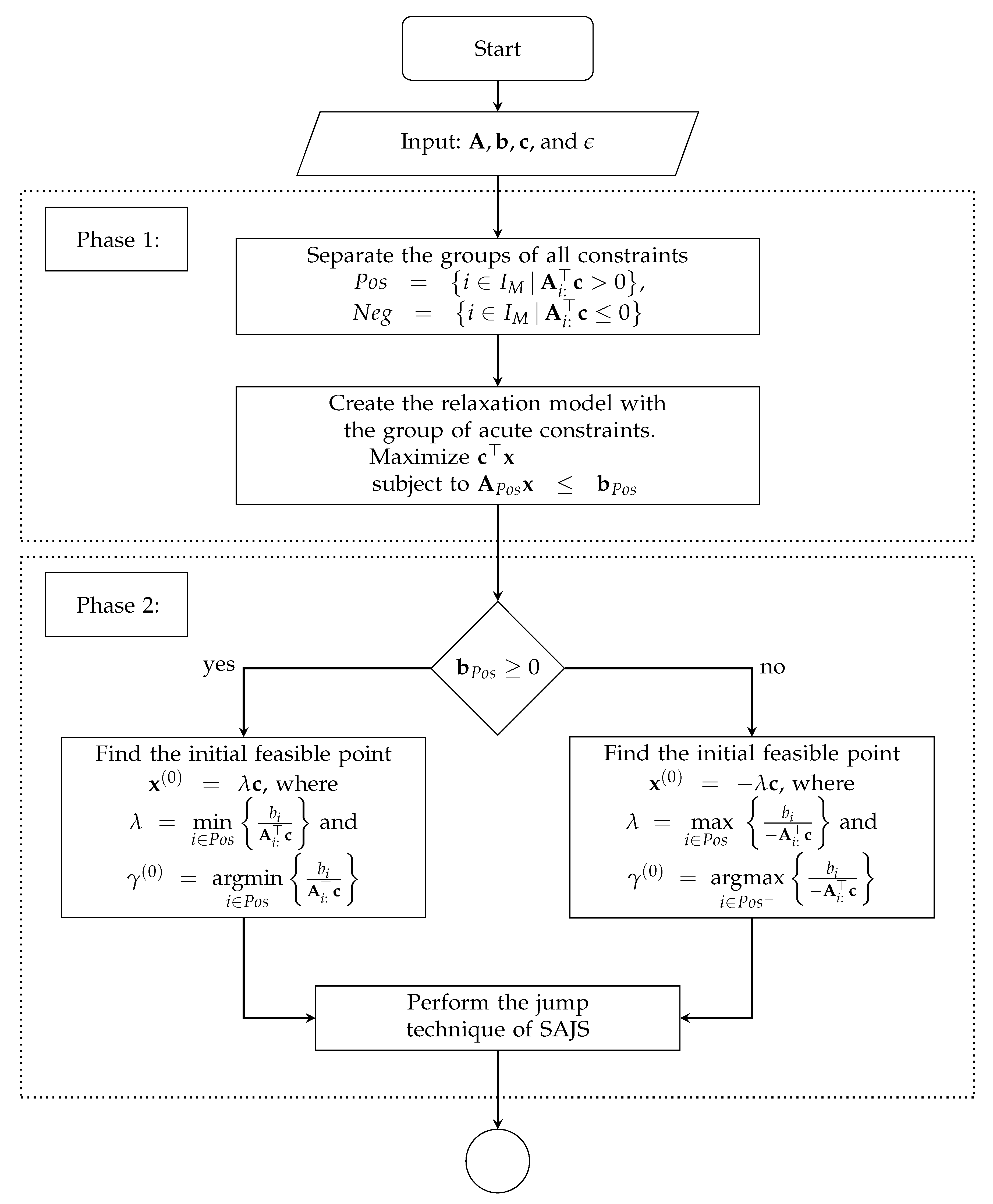
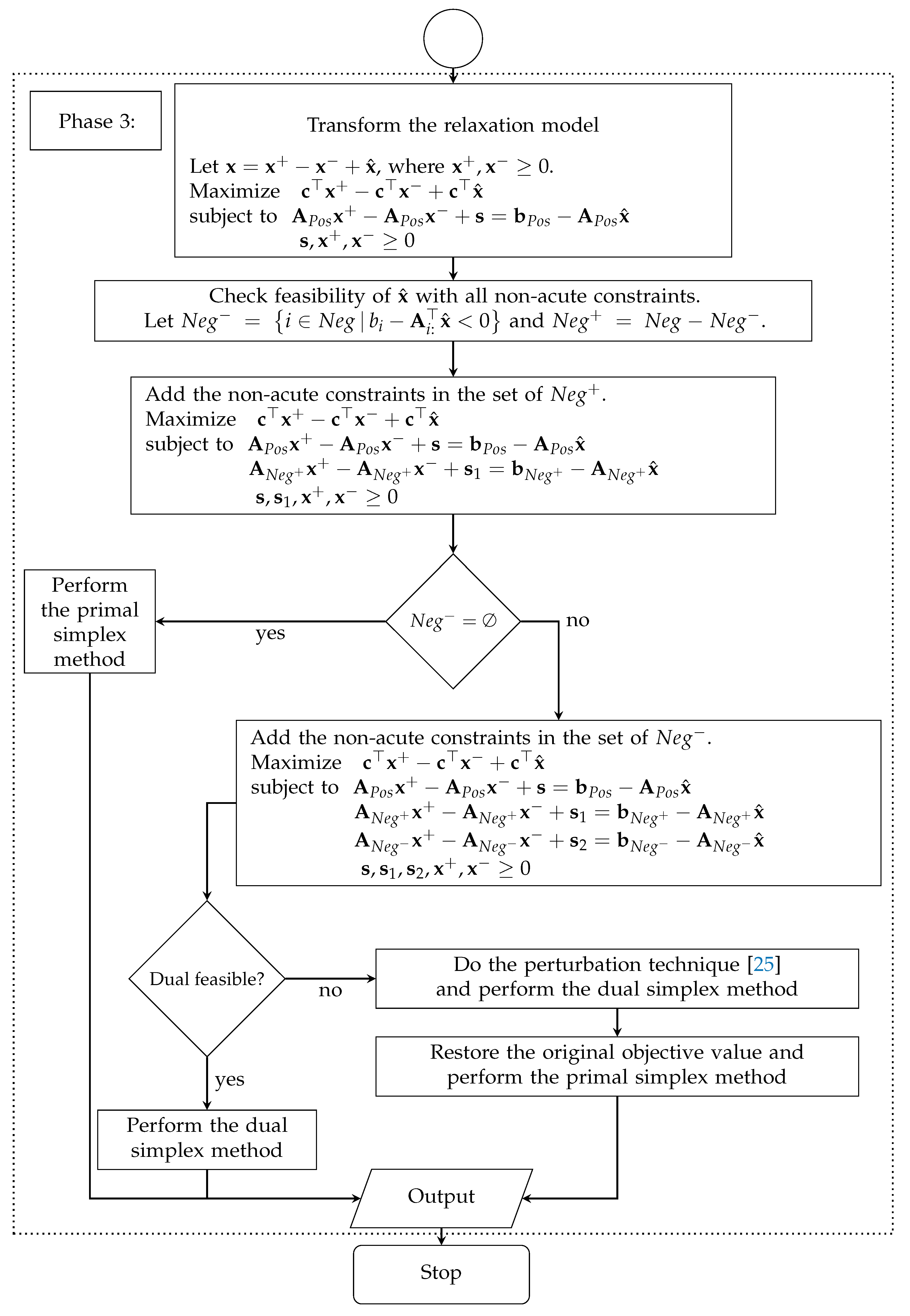
For this reason, a self-regulating artificial-free linear programming solver using jump and simplex method (SAJS) is proposed. It integrates the jump concept on a relaxation model similar to SNAR. SAJS consists of three phases. In phase 1, the relaxation model is created by a group of acute constraints. In phase 2, SAJS applies the technique of iterative jumps along the improving directions of the objective value. The non-acute constraints are restored, and SAJS finds the point using the dual simplex method on the perturbation model before applying the final simplex method in phase 3.
The idea of the iterative jump method uses the improvement direction according to the objective gradient vector, similarly to the gravitational method. However, SAJS combines this direction with the current gradient vector of binding constraints at the current point while the gravitational method drops along the faces at the current point. Moreover, SAJS is applied on the relaxation model before applying the dual simplex method at the last step while the gravitational method works on the original model.
This paper is divided into five parts. Section 2 details the preliminaries, while SAJS is explained in Section 3. In Section 4, experiments and results are shown. Finally, the conclusion is proposed in Section 5.

2. Background and Knowledge

Consider a linear program as follows:
Maximize c x subject to Ax b ,
where c is a nonzero vector in R n , x R n , A is an m × n matrix and b R m , and m > n . Let  I M = 1 , 2 , , m . SNAR [18] and preliminaries of SAJS are described in this section.

2.1. SNAR Description

SNAR starts with the relaxation model, consisting of a group of acute constraints corresponding to the objective gradient vector. Let A i : be a gradient vector of the i t h constraint from the matrix A , let  c be an objective gradient vector, and let θ i be defined as follows:
θ i = arccos A i : c A i : c .
Two separating groups of constraints can be considered from the sign of A i : c only, since  A i : c > 0 . Let P o s be a set of all acute constraints defined as P o s = i I M | A i : c > 0 , and let N e g be a set of all non-acute constraints defined as N e g = i I M | A i : c 0 .
After that, SNAR will create the relaxation model consisting of the group of acute constraints.
Maximize c x subject to A P o s x b P o s ,
where A P o s is a submatrix from the row indices from P o s , and b P o s is the column vector of constraints corresponding to P o s .
For model (3), SNAR uses the simplex method to find a solution. If b P o s 0 , then the simplex method can start at 0 . Otherwise, SNAR will define x ( 0 ) = λ c , where λ = max i P o s b i A i : c and P o s = { i P o s | b i < 0 } . For each x in model (3), let x ˜ = x x ( 0 ) . Thus, model (3) is relocated as follows:
Maximize c x ˜ + c x ( 0 ) subject to A P o s x ˜ b P o s A P o s x ( 0 ) .
Next, model (4) is the unrestricted model which is needed to transform to the standard form for the simplex method. First, the vector of slack variables s is added to all constraints, changing inequality constraints into equality constraints.
Maximize c x ˜ + c x ( 0 ) subject to A P o s x ˜ + s = b P o s A P o s x ( 0 ) s 0 .
Subsequently, let x ˜ = x + x , where x + , x 0 . Therefore, model (5) is converted before starting the simplex method.
Maximize c x + c x + c x ( 0 ) subject to A P o s x + A P o s x + s = b P o s A P o s x ( 0 ) s , x + , x 0 .
After the simplex method is complete, the result can be either optimal or unbounded optimal. For the case of the optimal solution, all constraints from N e g will be added into the model. If it is feasible after adding non-acute constraints, then the current solution is also the optimal solution of the original model. Otherwise, the dual simplex is performed in order to find the optimal solution. For the other case of the unbounded optimal solution, each non-acute constraint is restored in the relaxation model. The technique of Pan [25] is applied to change dual infeasible to dual feasible before performing the dual simplex method. The process of the unbounded will be repeated until the result of the relaxation model is optimal. Then, it returns to be performed in the case of the optimal solution.

2.2. Preliminaries of SAJS

The related theorems for establishing SAJS are shown in this section. Consider the relaxation model as follows:
Maximize c x subject to A P o s x b P o s .
To start at the more suitable point for model (7), SAJS considers two scenarios. If b P o s 0 , SAJS starts with x ( 0 ) = λ c , where λ = max i P o s b i A i : c , the same as SNAR. Otherwise, SAJS defines x ( 0 ) = λ c , where λ = min i P o s b i A i : c . The case in which b P o s 0 proved that x ( 0 ) is feasible in [18]. Another case will be proven in Theorem 1.
Theorem 1.
Given a linear program like that in model (7) and P o s = i I M | A i : c > 0 , if b P o s 0 and λ = min i P o s b i A i : c , where A i : is a gradient vector of the i t h constraint from the matrix A , then x ( 0 ) = λ c is feasible.
Proof. 
Suppose b P o s 0 and λ = min i P o s b i A i : c . Since b i 0 and A i : c > 0 for all i P o s , λ 0 . So, λ b h A h : c for all h P o s . Hence, λ A h : c b h . Choosing x ( 0 ) = λ c gives A h : x ( 0 ) b h for all h P o s . Thus, A P o s x ( 0 ) b P o s . □
After the initial feasible point of the relaxation model is found, SAJS will iteratively jump to other improved feasible points using the following theorem.
Theorem 2.
Given a linear program like that in model (7) with c 0 and P o s = i I M | A i : c > 0 , let x o l d be a feasible point which lies on the γ t h constraint of A , v = A γ : A γ : + c c , and
S = b i A i : x o l d A i : v i P o s and A i : v > 0 and b i A i : x o l d > 0 .
Suppose S and v 0 and let α = min S . Then, x n e w = x o l d + α v is feasible and c x o l d < c x n e w .
Proof. 
Let x o l d be a feasible point for model (7) which lies on the γ t h constraint, v = A γ : A γ : + c c , c 0 , and S = b i A i : x o l d A i : v i P o s and A i : v > 0 and b i A i : x o l d > 0 . Assume that S and v 0 . Let α = min S . Since x o l d is the feasible point, b t A t : x o l d 0 for all t P o s .
For t P o s , A t : v > 0 ,
α b t A t : x o l d A t : v A t : α v b t A t : x o l d A t : x o l d + α v b t A t : x n e w b t .
For t P o s , A t : v < 0 ,
b t A t : x o l d A t : v < α A t : α v < b t A t : x o l d A t : x o l d + α v < b t A t : x n e w < b t .
For t P o s , A t : v = 0 ,
A t : x n e w = A t : x o l d + α v = A t : x o l d b t .
Hence, A P o s x n e w b P o s .
Then, x n e w is the feasible point.
Next, it can be shown that c x o l d < c x n e w . Consider
c x n e w = c ( x o l d + α v ) = c x o l d + α c v .
Since
c v = c A γ : A γ : + c c = c A γ : A γ : + c 2 c = A γ : c cos θ A γ : + c = c 1 cos θ > 0 ( sin ce , 1 < cos θ < 1 )
and α > 0 , hence, c x o l d < c x n e w . □
SAJS enhances the performance of solving a linear program without using artificial variables and the user’s parameters. It consists of three phases. In phase 1, SAJS creates the relaxation model by relaxing all non-acute constraints to guarantee the existence of a feasible point.
In phase 2, SAJS applies the technique of iterative jumps to find a feasible point. For each jump, the objective value of the relaxation model is improved until it reaches the stopping criterion ( ϵ ). The stopping criterion is defined as the minimum ratio improvement of two consecutive differences of the objective values of SAJS. The appropriate setting for the stopping criterion is discussed in Section 4.
After phase 2 terminates, slack variables are added to transform the last jump point into the extreme point, initializing phase 3. SAJS divides the non-acute constraints into two groups: The non-acute constraints which the last jump point in phase 2 is satisfied and the non-acute constraints which the last jump point in phase 2 is violated. The non-acute constraints from the first group are reinserted into the model, maintaining the feasibility of the last jump point. Afterwards, the remaining non-acute constraints are reinserted into the model, and SAJS expands the current relaxation model to the standard form of the LP by adding the variables and constraints into the model.

3. The Process of SAJS

Consider a linear program in the following form:
Maximize c x subject to Ax b .
The flowchart of SAJS, comprised of 3 phases, is shown. Phase 1 is the construction of the relaxation model. Phase 2 performs the iterative jumps by Algorithm 1 along an improving direction. The procedure of phases 1 and 2 of SAJS are shown in Figure 3. It will stop when the ratio of consecutive differences for the objective values is less than the user’s stopping criterion, which will be explained in Section 4. After that, the model is transformed into the standard form, and the group of non-acute constraints is reinserted into the model in order to find the optimal solution of the original model in phase 3 as demonstrated in Figure 4. However, if the unbounded optimal solution is detected after the dual simplex method is performed, then SAJS concludes that the original model is infeasible.
Algorithm 1 Jump technique of SAJS
Input: A , b , c , x ( 0 ) , γ ( 0 ) , P o s , ϵ
Output: x ^
  1:Set k = 0 , Δ z ( 1 ) = Δ z ( 0 ) = 1 , where Δ z ( 1 ) and Δ z ( 0 ) are the initial values of the consecutive differences.
  2:while Δ z ( k + 1 ) Δ z ( k ) > ϵ do
  3:  Compute v = A γ ( k ) : A γ ( k ) : + c c , where c 0 .
  4:  Construct P o s = P o s \ { γ ( k ) } .
  5:  Set α = M , where M is a large constant.
  6:  for i P o s do
  7:    if A i : v > 0 and b i A i : x ( k ) > 0 then
  8:      Compute D i s t = b i A i : x ( k ) A i : v .
  9:      if D i s t < α then
10:        Define α = D i s t .
11:        Define γ ( k + 1 ) = i .
12:      end if
13:    end if
14:  end for
15:  if α M then
16:    Compute x ( k + 1 ) = x ( k ) + α v .
17:    Compute Δ z ( k + 1 ) = c x ( k + 1 ) c x ( k ) .
18:    Compute k = k + 1 .
19:  else
20:    break
21:  end if
22:end while
23:Set x ^ = x ( k + 1 )

4. Experiments and Results

The computational results of the wall-clock time of SAJS, the Two-Phase method, and SNAR on 41 standard problems from netlib and 280 randomly generated problems are presented in this section. The maximizing linear programs are randomly generated with the objective vector c , equal to a vector of ones, and the number of constraints is higher than the number of variables, which exhibits the worst-case performance of SNAR. Furthermore, these linear programs check for optimal solutions before they are included in the experiment. The experiments were performed by using an Intel(R) Core(TM) i7-3770 [email protected] GHz processor with 8 GB RAM on Windows 10. Three methods, SAJS, the Two-Phase method, and SNAR, were written by Python libraries numpy.
The rows of matrix A are generated in two groups. The first group is generated for row i = 1 , 2 , , k , where k = 3 4 n . All coefficients in this group of the matrix A are uniformly random from [ 3 , 9 ] , with a high probability of making acute angles with the objective vector. The second group is generated for row i = k + 1 , k + 2 , , m , with uniformly random coefficients from [ 9 , 3 ] and with a high probability of making obtuse angles with the objective vector. To guarantee a nonempty feasible region, the intended feasible solution vector x is generated first with x j [ 9 , 9 ] , j = 1 , 2 , , n , and then the vector’s right-hand side b is calculated from b i = A i : x , where i = 1 , 2 , , n , and b i = A i : x + 1 , where i = n + 1 , n + 2 , , m .
The randomly generated problems are simulated by their sizes with varying m constraints and n variables according to the following scenarios: m > n , m { 100 , 200 , 300 , 400 , 500 , 1000 , 2000 } , n m 10 , 2 m 10 , 3 m 10 , 4 m 10 . The wall-clock times of each of the sizes of the randomly generated problems are averaged by 10 different problems and are shown in Figure 5, Table 1, and Figure 6.
Figure 5 shows the average wall-clock time varying according to stopping criteria of 0.20, 0.30, 0.40, and 0.50, which are used in phase 2 of SAJS. The stopping criterion is defined as the minimum ratio improvement of two consecutive differences of the objective values of SAJS. However, the average wall-clock times (in seconds) of the computations for each stopping criterion are not significantly different. Thus, in this paper, SAJS uses ϵ = 0.40 to compare with the Two-Phase method and SNAR, which are presented in Figure 6 and Figure 7. The reason is that the average total wall-clock time of SAJS with ϵ = 0.40 surpasses those of other stopping criteria.
Table 1 shows the average wall-clock time of SAJS with ϵ = 0.40 to determine the longest time from these three phases: Row represents the number of rows of the LP model and Col represents the number of columns of the LP model. The values under phase 1, phase 2, phase 3, and total time are the actual wall-clock times of each phase. The values in the parentheses present the ratio of the wall-clock time of each phase to the total time. It can be observed that the actual times of phase 1 and phase 2 are very small with respect to the wall-clock time of phase 3. Hence, the largest proportion of the running time of SAJS originates from phase 3.
The comparison of SAJS with ϵ = 0.40, the Two-Phase method (TP), and SNAR using randomly generated problems is presented in Figure 6. The performance of SAJS outperforms both methods. Since adding artificial variables in Two-Phase method enlarges the LP model, the Two-Phase method requires longer computational time to find the solution. For SNAR, the construction of the relaxation models of the randomly generated problems requires the reinsertion of the non-acute constraints into the model one by one, which takes a long time to find the solution. Moreover, Figure 6 shows that both the number of variables and the number of constraints affect the wall-clock time of SNAR.
Figure 7 demonstrates the performance computation of SAJS with ϵ = 0.40 , the Two-Phase method (TP), and SNAR using standard test problems from real-world netlib problems. m × n represents the dimension of the LP model. In this paper, the maximum time limit of computation is set to one day, which is equivalent to 86,400 s. However, the results with wall-clock times that exceed this limit will not appear in the figure; these include SCSD6, SCSD8, 25FV47, SCFXM3, SHIP08S, DEGEN3, SHIP12S, and SHIP08L. The efficacies of the three methods are comparable for small LP models with a number of variables times constraints of less than 30,000, from AFIRO to ADLITTLE. When LP models have of a number of variables times constraints of greater than 30,000, SNAR exhibits poor performance, with the exception of BRANDY, SCTAP1, SCTAP2, and SCTAP3, which have similar performance with SAJS due to the discovery of the optimal point in the relaxation model. For LP models with a number of variables times constraints of greater than 200,000 from SCTAP1 to SHIP08L, SAJS outperforms the Two-Phase method and SNAR, except with SCTAP2. The Two-Phase method has a lower performance when the LP model contains a large number of constraints and variables because the Two-Phase method takes a long time to handle all constraints. On the contrary, SAJS and SNAR start with the relaxation model, dealing with a smaller model. When the solution of the relaxation model is unbounded optimal, SNAR exhibits poor performance compared to other methods due to the reinsertion of the non-acute constraints one by one. The nonparametric Wilcoxon test is used to verify the effectiveness of SAJS against TP and SAJS against SNAR. The p-value of difference between SAJS and TP from the Wilcoxon signed rank test is equal to 0.003198, while the p-value of difference between SAJS and SNAR is equal to 3.30828 × 10 6 . Hence, SAJS statistically significantly outperforms both TP and SNAR.

5. Conclusions

This paper proposes a new self-regulating artificial-free method for solving a linear program, namely SAJS. The three phases of SAJS are the established relaxation model phase (phase 1), the jump phase to find the suitable initial point (phase 2), and the phase of reinsertion of non-acute constraints (phase 3). The relaxation model is created in phase 1 in order to guarantee the existence of a feasible point. The jump technique in phase 2 applies the technique of iterative jumps along the improving directions of the objective value, avoiding extreme points formed by acute constraints. In phase 3, the technique of reinsertion of non-acute constraints restores the group of non-acute constraints to the model.
Improving the solution time of the simplex method is still an active research area, appearing in various publications. The simplex method starts with the initial basic feasible solution before pivoting to the better alternative ones. For a general linear programming problem, the starting initial basic feasible solution is identified by enlarging the dimension of the decision variables, as in the two-phase method. Our method counters this issue by working on the feasible region with a small number of extreme points and avoiding extreme points using the jump technique, which significantly reduces the solution time of the simplex method. Nevertheless, if a linear programming problem has no “greater than or equal to” constraint, this improvement may not be significantly obvious.
Adding the artificial variable into the small-sized model rarely affects solving LP model for the Two-Phase method, whereas adding artificial variables to the large-sized model will have a significant effect on computational time. This does not affect SNAR or SAJS. Moreover, both methods begin with the relaxation model, so the size of the problem will be small. Hence, the performance of the Two-Phase method is inferior to those of both SNAR and SAJS for the large-sized model, though it is comparable with both for the small-sized model.
If the solution of the relaxation model is unbounded, the non-acute constraints will be reinserted into the LP model one by one. This affects the performance of SNAR, while SAJS reinserts two collections of the non-acute constraints at one time and performs the dual simplex method to reach the optimal solution. Therefore, for all randomly generated problems, SAJS outperforms other methods for all problem sizes.
To verify the effectiveness of SAJS, the nonparametric Wilcoxon test is performed on the standard test problems from netlib. SAJS exhibits significantly better overall performance over both the Two-Phase method and SNAR. Nevertheless, after comparing the wall-clock times of all three phases, it is clearly shown that SAJS takes a very short time in phase 1 and phase 2, while it spends almost the entire running time in phase 3 to find the solution by the dual simplex method.
In future work, the appropriate jumping direction of SAJS should be investigated. Moreover, other pivot rules of the dual simplex method in the reinsertion phase may improve the overall performance of SAJS.

Author Contributions

Conceptualization, R.V., K.S., and A.-a.B.; methodology, R.V., K.S., and A.-a.B.; software, R.V. and K.S.; validation, R.V., K.S., and A.-a.B.; formal analysis, K.S.; investigation, K.S. and A.-a.B.; writing—original draft preparation, R.V.; writing—review and editing, K.S. and A.-a.B.; visualization, R.V.; supervision, K.S.; project administration, K.S. All authors have read and agreed to the published version of the manuscript.

Acknowledgments

This research is supported by the Science Achievement Scholarship of Thailand and the Applied Mathematics and Computational Science Program in the Department of Mathematics and Computer Science, Faculty of Science, Chulalongkorn University, Thailand. The authors would like to thank Chittima Chiamanusorn and Thitiwat Piyatamrong for their valuable comments and suggestions.

Conflicts of Interest

The authors declare no conflict of interest.

Abbreviations

The following abbreviations are used in this manuscript:
LPLinear program
SNARArtificial-free simplex algorithm based on the non-acute constraint relaxation
SAJSSelf-regulating artificial-free linear programming solver using a jump and simplex method
TPTwo-Phase method
ϵ The stopping criterion

References

  1. Klabjan, D.; Johnson, E.L.; Nemhauser, G.L.; Gelman, E.; Ramaswamy, S. Solving large airline crew scheduling problems: Random pairing generation and strong branching. Comput. Optim. Appl. 2001, 20, 73–91. [Google Scholar] [CrossRef]
  2. Marsten, R.E.; Shepardson, F. Exact solution of crew scheduling problems using the set partitioning model: Recent successful applications. Networks 1981, 11, 165–177. [Google Scholar] [CrossRef]
  3. Wedelin, D. An algorithm for large scale 0–1 integer programming with application to airline crew scheduling. Ann. Oper. Res. 1995, 57, 283–301. [Google Scholar] [CrossRef]
  4. Hanssmann, F.; Hess, S.W. A linear programming approach to production and employment scheduling. Manag. Sci. 1960, 1, 46–51. [Google Scholar] [CrossRef]
  5. Anderson, A.M.; Earle, M.D. Diet planning in the third world by linear and goal programming. J. Oper. Res. Soc. 1983, 34, 9–16. [Google Scholar] [CrossRef]
  6. Kim, J.S.; Jeon, E.; Noh, J.; Park, J.H. A model and an algorithm for a large-scale sustainable supplier selection and order allocation problem. Mathematics 2018, 6, 325. [Google Scholar] [CrossRef] [Green Version]
  7. Dantzig, G.B. Linear Programming and Extensions; Princeton University Press: Princeton, NJ, USA, 1963. [Google Scholar]
  8. Karmarkar, N. A new polynomial-time algorithm for linear programming. Combinatorica 1984, 4, 373–395. [Google Scholar] [CrossRef]
  9. Murty, K.G. The gravitational method for linear programming. Opsearch 1986, 23, 206–214. [Google Scholar]
  10. Arsham, H. An artificial-free simplex-type algorithm for general LP models. Math. Comput. Model. 1997, 25, 107–123. [Google Scholar] [CrossRef]
  11. Arsham, D.H. Initialization of the simplex algorithm: An artifical-free approach. SIAM Rev. 1997, 39, 736–744. [Google Scholar] [CrossRef]
  12. Enge, A.; Huhn, P. A counterexample to H. Arsham’s “initialization of the simplex algorithm: An artificial-free approach”. SIAM Rev. 1998, 40, 1–8. [Google Scholar]
  13. Gao, P. Improvement and its computer implementation of an artificial-free simplex-type algorithm by Arsham. Appl. Math. Comput. 2015, 263, 410–415. [Google Scholar] [CrossRef]
  14. Junior, H.V.; Lins, M.P.E. An improved initial basis for the simplex algorithm. Comput. Oper. Res. 2005, 32, 1983–1993. [Google Scholar] [CrossRef]
  15. Arsham, D.H. Big-M free solution algorithm for general linear programs. J. Pure Appl. Math. 2006, 32, 549–564. [Google Scholar]
  16. Arsham, H. A computationally stable solution algorithm for linear programs. Appl. Math. Comput. 2007, 188, 1549–1561. [Google Scholar] [CrossRef]
  17. Corley, H.; Rosenberger, J.; Yeh, W.C.; Sung, T. The cosine simplex algorithm. Int. J. Adv. Manuf. Tech. 2006, 27, 1047–1050. [Google Scholar] [CrossRef]
  18. Boonperm, A.; Sinapiromsaran, K. Artificial-free simplex algorithm based on the non-acute constraint relaxation. Appl. Math. Comput. 2014, 234, 385–401. [Google Scholar] [CrossRef]
  19. Imtiaz, M.; Touheed, N.; Inayatullah, S. Artificial free clone of simplex method for feasibility. arXiv 2013, arXiv:1304.6894. [Google Scholar]
  20. Inayatullah, S.; Touheed, N.; Imtiaz, M. A streamlined artificial variable free version of simplex method. PLoS ONE 2015, 10, e0116156. [Google Scholar] [CrossRef] [Green Version]
  21. Arsham, D.H.; Damij, T.; Grad, J. An algorithm for simplex tableau reduction: The push-to-pull solution strategy. Appl. Math. Comput. 2003, 137, 525–547. [Google Scholar] [CrossRef]
  22. Arsham, H.; Adlakha, V.; Lev, B. A simplified algebraic method for system of linear inequalities with LP applications. Omega 2009, 37, 876–882. [Google Scholar] [CrossRef]
  23. Luh, H.; Tsaih, R. An efficient search direction for linear programming problems. Comput. Oper. Res. 2002, 29, 195–203. [Google Scholar] [CrossRef]
  24. Al-Najjar, C.; Malakooti, B. Hybrid-LP: Finding advanced starting points for simplex, and pivoting LP methods. Comput. Oper. Res. 2011, 38, 427–434. [Google Scholar] [CrossRef]
  25. Pan, P. Primal perturbation simplex algorithms for linear programming. J. Comput. Math. 2000, 18, 587–596. [Google Scholar]
Figure 1. Simplex method for SNAR (artificial-free simplex algorithm based on the non-acute constraint relaxation).
Mathematics 08 00356 g001
Figure 2. Iterative jumps from SAJS (self-regulating artificial-free linear programming solver using a jump and simplex method).
Mathematics 08 00356 g002
Figure 3. The flowchart of SAJS showing phase 1 and phase 2.
Mathematics 08 00356 g003
Figure 4. The flowchart of SAJS showing phase 3.
Mathematics 08 00356 g004
Figure 5. SAJS performances by varying the stopping criterion.
Mathematics 08 00356 g005
Figure 6. The comparison of SAJS, the Two-Phase method (TP), and SNAR using the average wall-clock time—randomly generated linear programming problems.
Mathematics 08 00356 g006
Figure 7. The comparison of SAJS, TP, and SNAR using the average wall-clock time—netlib problems.
Mathematics 08 00356 g007
Table 1. The average wall-clock time of SAJS with ϵ = 0.40.
RowColTime (s)Total Time
Phase 1Phase 2Phase 3
100100.0020 (0.0863)0.0003 (0.0132)0.0205 (0.9006)0.0228
100200.0005 (0.0115)0.0074 (0.1701)0.0356 (0.8184)0.0435
100300.0021 (0.0322)0.0039 (0.0597)0.0593 (0.9081)0.0653
100400.0025 (0.0293)0.0024 (0.0281)0.0805 (0.9426)0.0853
200200.0009 (0.0080)0.0009 (0.0080)0.1113 (0.9841)0.1131
200400.0024 (0.0119)0.0042 (0.0209)0.1943 (0.9671)0.2009
200600.0075 (0.0219)0.0061 (0.0178)0.3291 (0.9603)0.3427
200800.0065 (0.0134)0.0113 (0.0233)0.4671 (0.9633)0.4848
300300.0053 (0.0169)0.0018 (0.0058)0.3058 (0.9773)0.3129
300600.0047 (0.0079)0.0047 (0.0079)0.5828 (0.9841)0.5922
300900.0068 (0.0058)0.0108 (0.0093)1.1491 (0.9849)1.1668
3001200.0076 (0.0044)0.0259 (0.0150)1.6965 (0.9806)1.7300
400400.0031 (0.0041)0.0031 (0.0041)0.7439 (0.9917)0.7501
400800.0090 (0.0053)0.0114 (0.0067)1.6839 (0.9880)1.7043
4001200.0125 (0.0047)0.0234 (0.0089)2.6007 (0.9864)2.6366
4001600.0139 (0.0038)0.0597 (0.0163)3.5919 (0.9799)3.6655
500500.0019 (0.0014)0.0112 (0.0080)1.3827 (0.9906)1.3954
5001000.0113 (0.0035)0.0234 (0.0073)3.1722 (0.9892)3.2070
5001500.0157 (0.0032)0.0437 (0.0088)4.8884 (0.9880)4.9479
5002000.0156 (0.0022)0.0890 (0.0124)7.0888 (0.9855)7.1935

