1. Introduction
The new informational aspects of our life allow us to imagine and realize the mechanisms of influences on society’s members and their opinions on some political and other social events. We can also assume that that the level of influence may be regulated by centers of influence in different ways (e.g., increasing the costs on advertisement policies, political debates, etc.). Different centers of influence may want to obtain opposite opinions or various levels of opinions on some event and the process to obtain these opinions among the members of the society becomes a competition. We propose several models with one or two players who compete for the opinion of society members based on DeGroot’s model of information diffusion [
1], in which the opinion dynamic is described as a dynamic process where agents or society members can influence each other’s opinions with a given intensity rate at any discrete time.
The models of finding a consensus are close to the models of informational influence on population and information control models (see, e.g., papers [
2,
3] and books [
4,
5]). A model of opinion dynamics with two principals or centers of influence is presented in [
6], in which the conditions of existence of the limit opinions are obtained for a given matrix of influences. The problem of reaching a consensus can be modeled as a repeated game [
7] or mean field game [
8]. There are also imitation models of opinion dynamics [
9]. The competitive and cooperative models of opinion dynamics are also considered in [
10,
11], in which the dynamic games of opinion formation are linear-quadratic. The authors find the equilibria representing the level of influence with different information structures (open-loop and closed-loop).
We introduce the models of opinion dynamics when agents, being the members of the network, form their opinions by the influence of the average opinion of the society. The averaging society opinion is considered as a natural way to represent a global trend in the present communities [
12]. Besides the agents who form the social network, there are one or two centers of influence which are interested in making the opinion of any player as close as possible to the target one. First, we consider an optimization problem with one player (a unique center of influence) minimizing costs that also depend on the level of influence. In this case, there are only two agents in the network, one of them is directly influenced by the player and the other one is influenced by the player via the opinion of the first agent. Second, we introduce a model of opinion dynamics with two players and two agents in the social network. Each player influences the opinion of the corresponding agent directly and the other agent’s opinion indirectly. Players are willing to minimize quadratic costs, trying to make the agents’ opinions closer to the target ones. We use the Nash equilibrium as a solution concept to solve the game. Third, we extend the previous model to the case when there are many agents and two players and the agents are divided into two groups by the influence of a particular player.
A social network defined by a set of agents described as the nodes in a network which is called a star is examined in [
13]. In that paper, the agents of the society communicate within the network and form opinions by influence of other society members who have direct links with them in the network. Agents cannot vary the intensity of influence over time. We assume that intensities are defined in a given matrix. In a star graph, one agent is centered and all non-central agents have a unique link connecting these agents with the center. The agents which are located not in the center of the network are assumed to be identical with their influential power on the central agent. The communication graph with a star structure can describe the small social networks in any company or office when there exists one head [
14]. Models using game theory ideas describing the network structures are considered in [
15]. In the case where the network has a lot of nodes, which can be difficult to examine, first the problem of partitioning the nodes is applied (see such models in [
16,
17]).
In all models presented in the paper, the state of the system considered in discrete time is defined by a profile of the opinions of the social network members. The dynamics of the state variable are given by a linear equation subject to the state in the previous period and players’ intensities of influence. The players’ costs are linear-quadratic functions with respect to the state variables and players’ strategies; therefore, the game we model is a linear-quadratic difference game. See [
18,
19] for a detailed analysis of the results on LQ games. The Euler-equation approach to find the solutions in such a class of games is considered in [
20]. In our paper, we first use the Euler-equation approach for the problems of opinion dynamics. This approach allows to find optimal or equilibrium strategies in a simpler way in comparison with Pontryagin’s maximum principle. In numerical simulation made for the paper, the Euler-equation approach demonstrates better results in working time, especially, when the number of periods is large.
The rest of the paper is organized as follows. We describe the Euler-equation approach in
Section 2. In
Section 3, we describe the optimization model with the given average-oriented opinion dynamics.
Section 4 contains the main result for the case of two agents and one player and finds the optimal strategy of the player optimal opinion trajectory in an explicit way. Then we introduce a game-theoretical model of competition for agents’ opinion in
Section 5. An extension of this model on the case of many agents is presented in
Section 6. We briefly conclude in
Section 7.
2. The Euler-Equation Approach
Let
and
be the state space and the control set, respectively. The state of a system evaluates with respect to dynamics
with initial state
. The optimal control problem is to find a control
maximizing Functional
with respect to the state dynamics Equations (
1) and a given initial condition
.
We can reformulate this problem in terms of the state trajectory
. Suppose that we can express
from Equation (
1) as a function of
and
, say
. Therefore, we can rewrite Functional (
2) in the following form:
where
,
.
The Euler equation approach gives the necessary conditions (see [
20,
21,
22]) for the optimal trajectory
:
We can notice that games considered in the paper belong to the class of linear-quadratic games, so the necessary conditions will be also sufficient conditions. We will apply the Euler-equation method to find the optimal strategies in the dynamic games with average-oriented opinion dynamics.
3. Optimization Problem
We consider a society consisting of
n agents. Each agent
i has an opinion
,
. The agents communicate with each other and change the opinion over time, which is assumed to be discrete and finite. Let opinion of agent
i at time
t be
,
. We also assume that there exists a player who influences the opinion of one particular agent, say agent 1 with intensity
at time
. In period
T the player does not influence the agent’s opinion. The opinion of agent 1 changes depending on his own opinion, the average opinion of the society and influence of the player. The opinion of any agent
changes over time depending on his own opinion and the average opinion of the society. The opinion dynamics is defined by the following equations:
with initial condition
In Equations (
5) and (6), constants
,
show the beliefs of agents to the average opinion of the society. The higher the average opinion, the higher the opinion of the agent at next time period.
Let the player aim in taking the opinion of all agents around some particular level
minimizing the total costs which are
where
is a discount factor and
is the player’s costs per unit of influence intense.
4. Case of Two Agents and One Player
For simplicity, we first consider the problem when the society consists of two agents and the opinion of agent 1 is influenced by the player. Therefore, we have the dynamics equations:
with initial condition
The dynamics equations may be rewritten in the following form:
with the same initial conditions.
The optimization problem for the player is to minimize the functional
The following theorem provide conditions to find the optimal strategy
minimizing Functional (
12) subject to initial Conditions (
9) and the state dynamics of Systems (
10) and (
11).
Theorem 1. Let be the optimal strategy minimizing Functional (
12)
subject to initial conditions (
9)
and state dynamics Equations (
10)
and (
11)
and be the corresponding state trajectory, then the optimal strategy , isand corresponding optimal state trajectory , is satisfied to equations:where , , , and . Proof of Theorem 1. For simplicity, we introduce a new variable
as
Then, we rewrite state equations in the following way:
with initial conditions
,
. Notice that
.
For using the method of Euler’s equations, we find the expression of
from Equation (
14) and substitute it to Functional (
3) and obtain
The function
is convex in
z,
. So, the minimum of this function under condition given by Equation (15) always exists. We form the Lagrange function
and write the first order conditions
,
and
,
, we obtain the system of equations:
with initial conditions
,
.
Excluding
from System (
16) we obtain
where
,
.
The theorem is proved. □
Remark 1. The Euler equation approach used to prove Theorem 1 and further Theorems 2 and 3 can be called an inverse method of solving the optimal control problems. System (13) in Theorem 1 is solved with respect to the state variable, i.e., the solution gives the optimal trajectory, and corresponding optimal controls are found in a unique way from the optimal state trajectory. This approach can be used only if the control or strategy can be represented as a function of state variables.
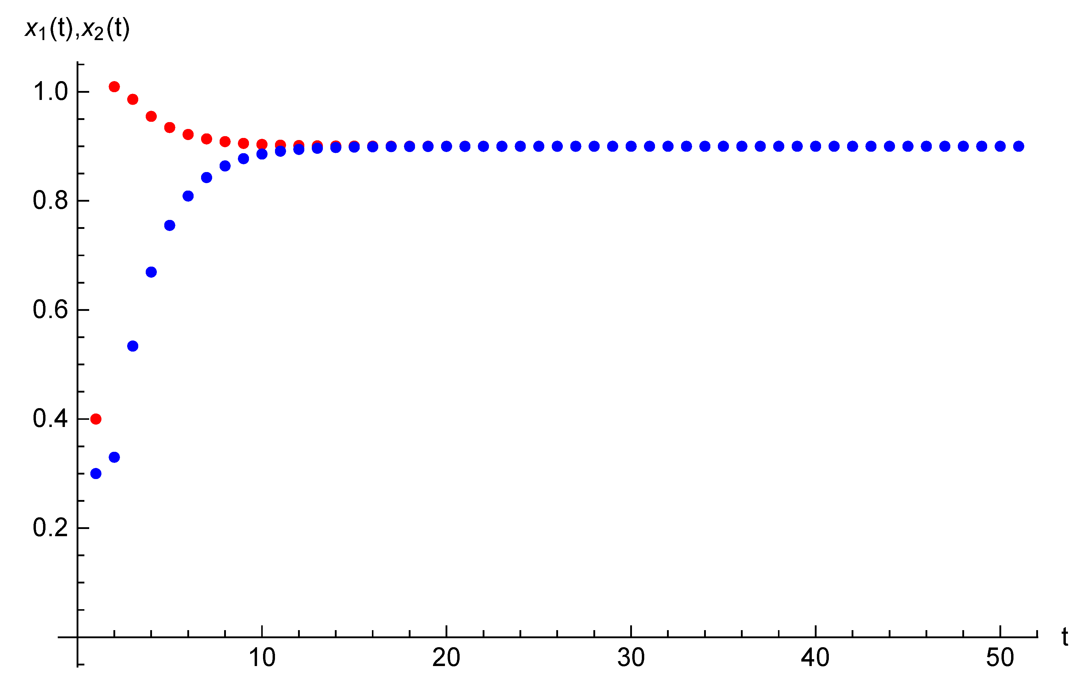
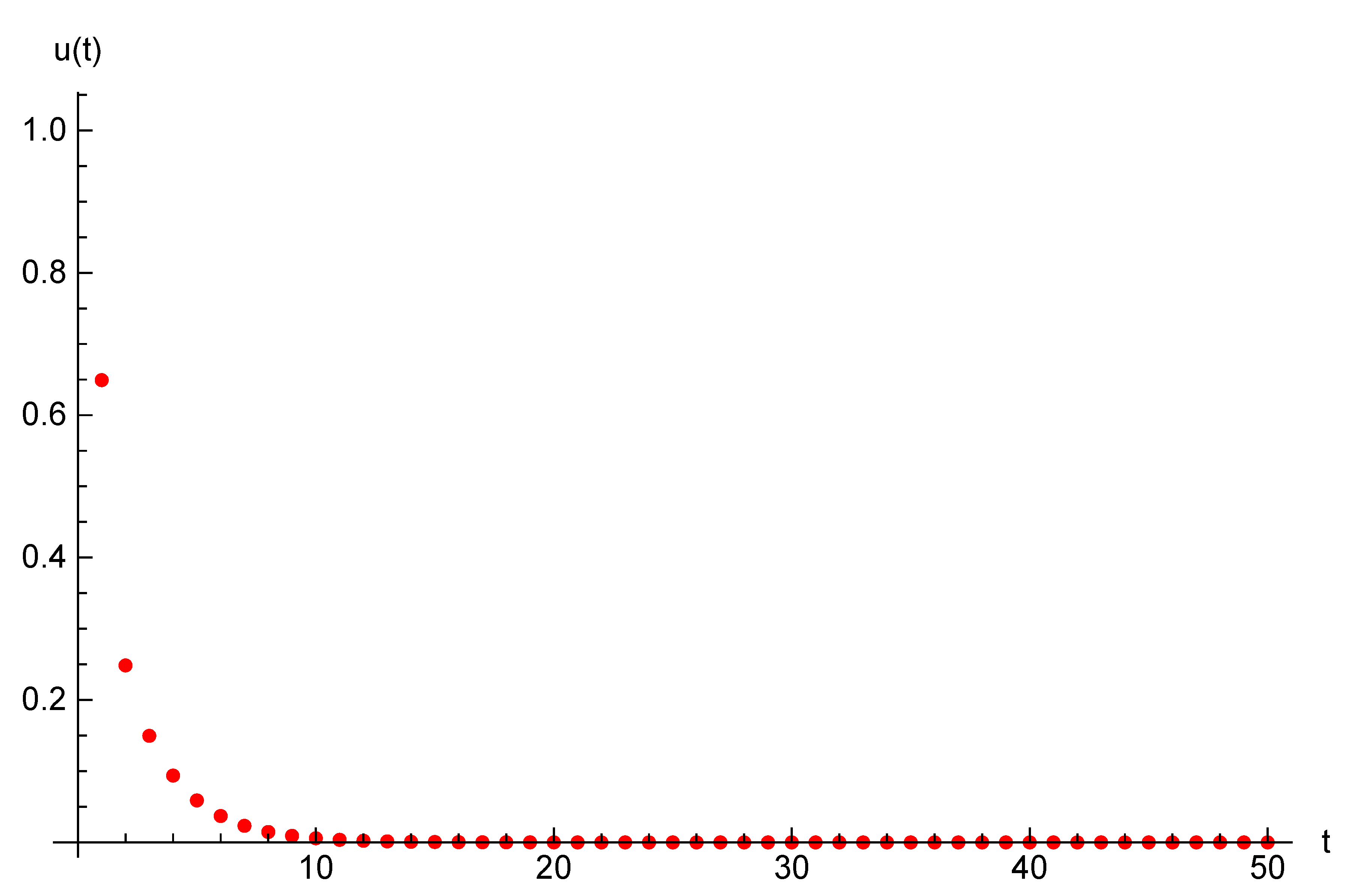
Example 1. Let the parameters of the optimal control problem be following: and initial opinions be , . For time horizon and target opinion , the optimal trajectory and optimal control are presented in Table 1. The optimal value for Functional (
3)
is . For the same parameters and duration we introduce state trajectories and strategy trajectory on Figure 1 and Figure 2. 5. Case of Two Agents and Two Players
Now we consider the case of competition on agents’ opinions. In comparison with the model described above, we assume that there are two players and one of them directly influences agent 1 and the other one—agent 2. The players have the same discount factors but they are different in their costs per unit of influence intense ( and ) and target opinion levels ( and ).
The state equations for opinions of agents 1 and 2 are
with initial Condition (
9).
Players 1 and 2 are willing to minimize the functionals
correspondingly, where
is player
i’s costs per unit of influence intensity.
We can define a two-player game in normal form representation with the set of players’ strategies
,
, where
,
, players’ cost functions
,
, defined by Formulas (
19) and (
20) s.t. state Equations (
17) and (
18) with initial state
. The game belongs to the class of linear-quadratic games.
The Nash equilibrium is used as an optimality principle or solution of the game with profile of strategies
s.t. the inequalities
hold for any
and
.
Let us fix
and find the best response of Player 1. We use the Euler-approach to find the Nash equilibrium in the game described. First, we find expressions of
from state Equation (
17) as a function of
and
and
from state Equation (18) as a function of
and
:
The goal of the first player is to minimize
subject to Condition (
18). We form the Lagrange function
where
. Finding the derivatives
and
,
and equating them to zero, we obtain the corresponding systems:
From the first equation of System (
21) we obtain
Denoting
and substituting it to System (
22) and taking into account the second equation in System (
21), we obtain the system of equations to define the best response strategy of Player 1:
where
We determine the best response strategy of Player 2 in the same way.
The following theorem gives the necessary conditions of the Nash equilibrium for the game described above.
Theorem 2. Let be the Nash equilibrium in the game and be the state trajectory corresponding to this equilibrium with initial condition , , then they satisfy the system:where andtaking into account the state Equations (
17)
and (
18)
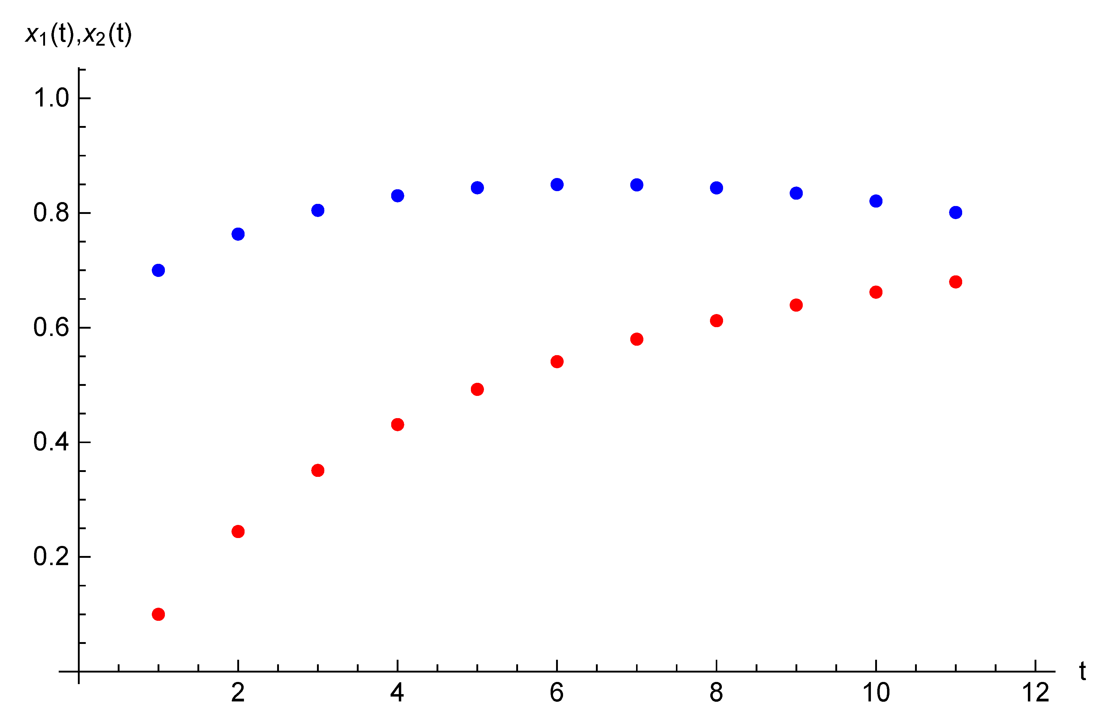
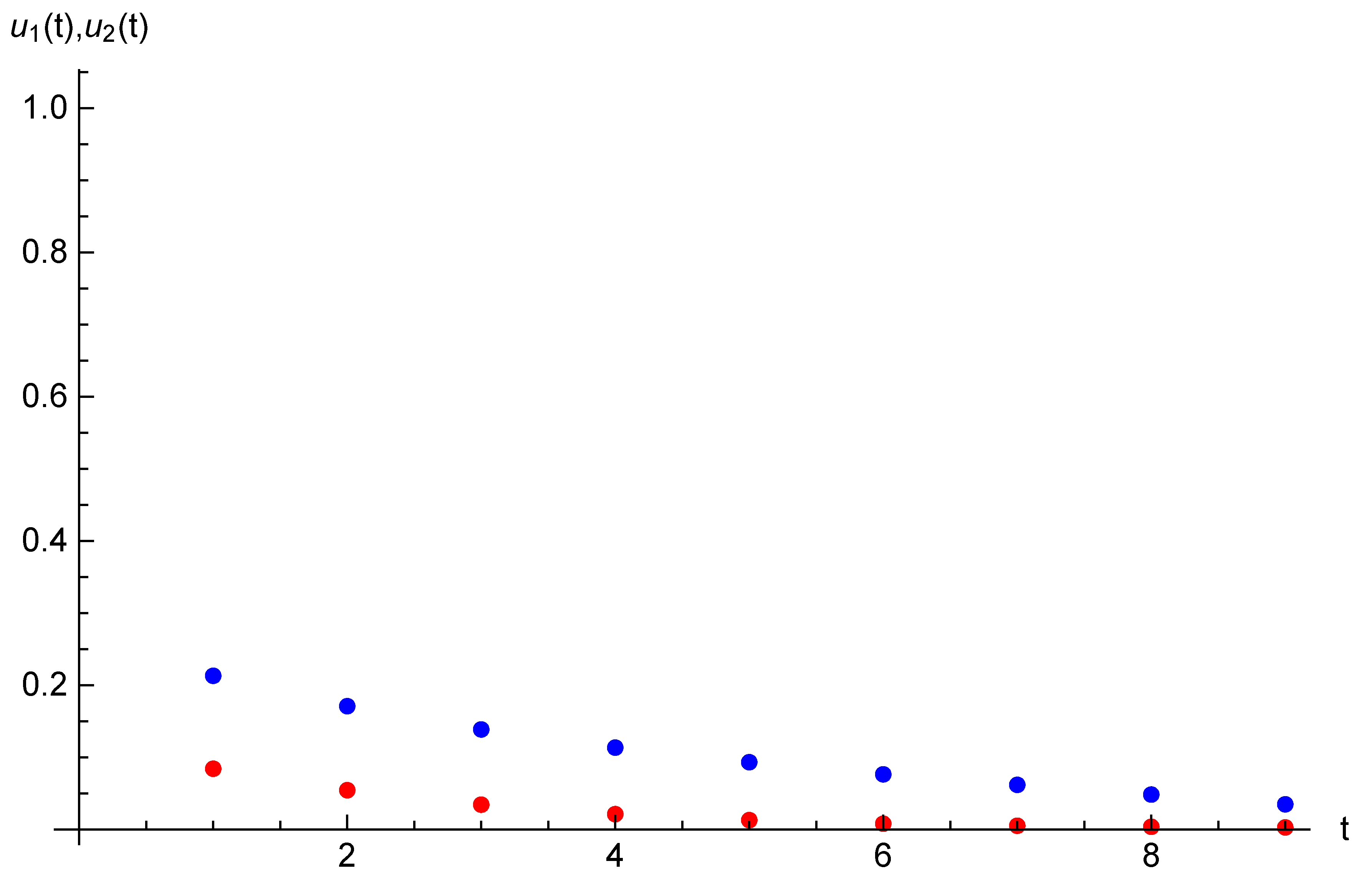
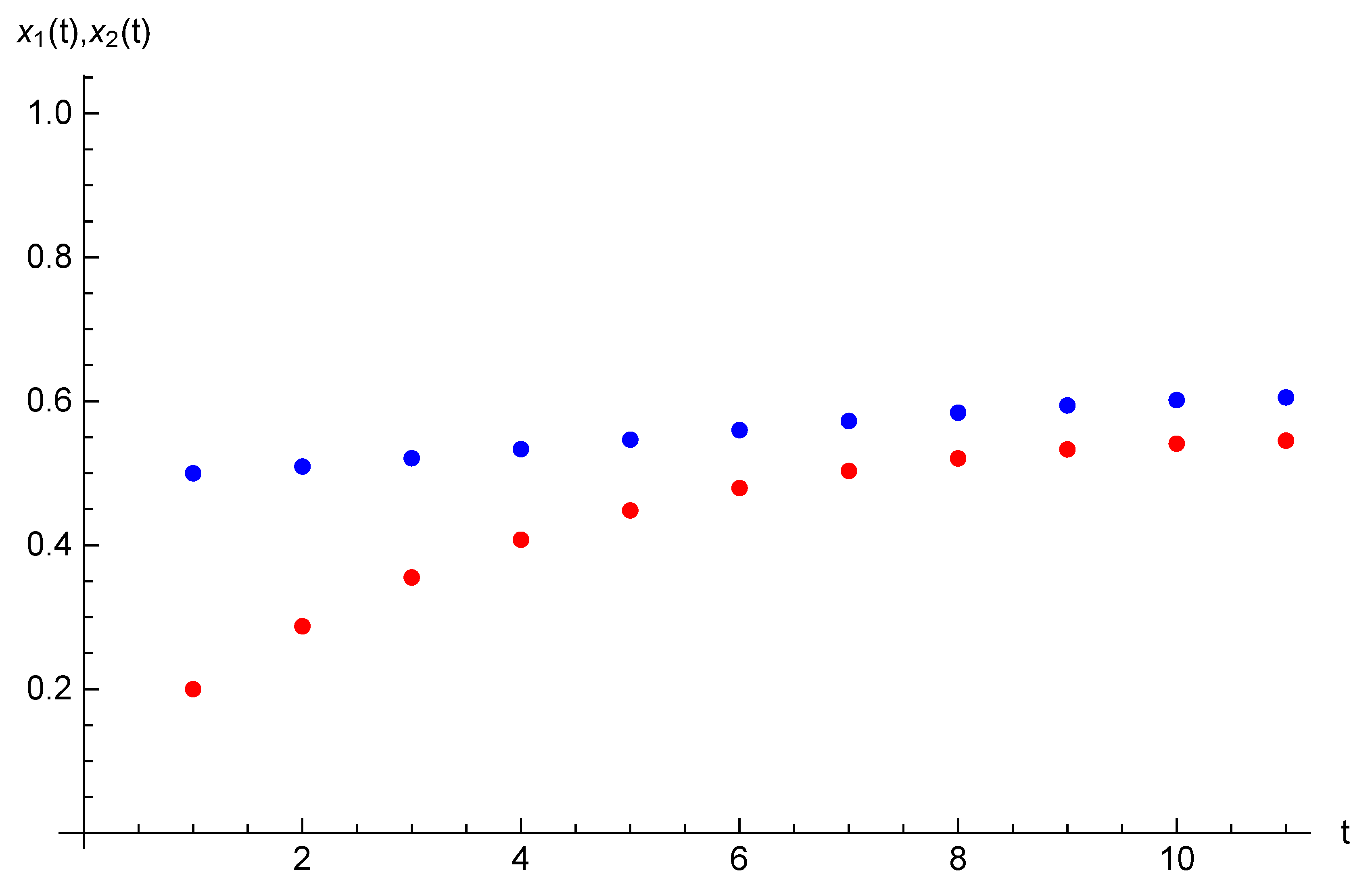
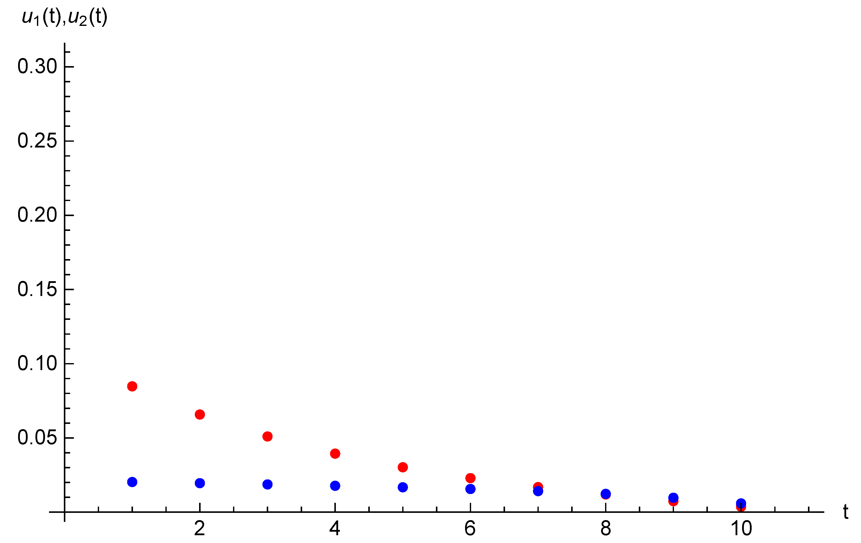
and initial state , . Example 2. Let the parameters of the game considered in this section be the following: , , and initial opinions be , . For time horizon , target opinions are , . The equilibrium state and strategy trajectories are presented on Figure 3 and Figure 4. The equilibrium costs of Players 1 and 2 are and , respectively. 6. Case of Many Agents and Two Players
In this section we extend the model introduced in
Section 4 on the case when there are more than two agents. The finite set of agents is divided into two groups. The first group contains agent 1 whose opinion is influenced by the average opinion of the society and Player 1. The second group contains
n identical agents whose opinion is influenced by the average opinion of the society and Player 2. All agents in the second group have unique initial opinion. The dynamics of agents’ opinions is given by equations
with initial condition
and
. As the agents 2,
…,
are identical, then we obtain that
for any
i and
and any
.
Players 1 and 2 are willing to minimize the functionals
correspondingly.
Thus, we define two-player game in a normal form with the set of players’ strategies
,
, where
,
, cost functions of the players
,
given by Functionals (
26) and (
27) s.t. state Equations (
24) and (
25) with initial state
. The game belongs to the class of linear-quadratic games.
The following theorem gives the necessary conditions of the Nash equilibrium for the game described above.
Theorem 3. Let be the Nash equilibrium and , where be the corresponding state trajectory with initial condition , , then they satisfy the system:where andtaking into account the state Equations (
24)
and (
25)
and initial state , . Proof of Theorem 3. First, we fix
and find the best response of Player 1. Using the Euler-approach to find the Nash equilibrium in the game described, we find expressions of
from state Equation (
24) as a function of
,
,
…,
and
from state Equation (25) as a function of
:
The goal of the first player is to minimize
subject to Equation (25). We form the Lagrange function
where
. Finding the derivatives
and
,
,
and equating them to zero, and taking into account the symmetry of agents 2,
…,
, we obtain the corresponding systems:
From the first equation of System (
29) we obtain
Denoting
and substituting it to Equation (
30) and taking into account the second equation in System (
29), we obtain the system of equations to define the best response strategy of Player 1:
where
We determine the best response strategy of Player 2 in the same way and obtain the System (
28). □
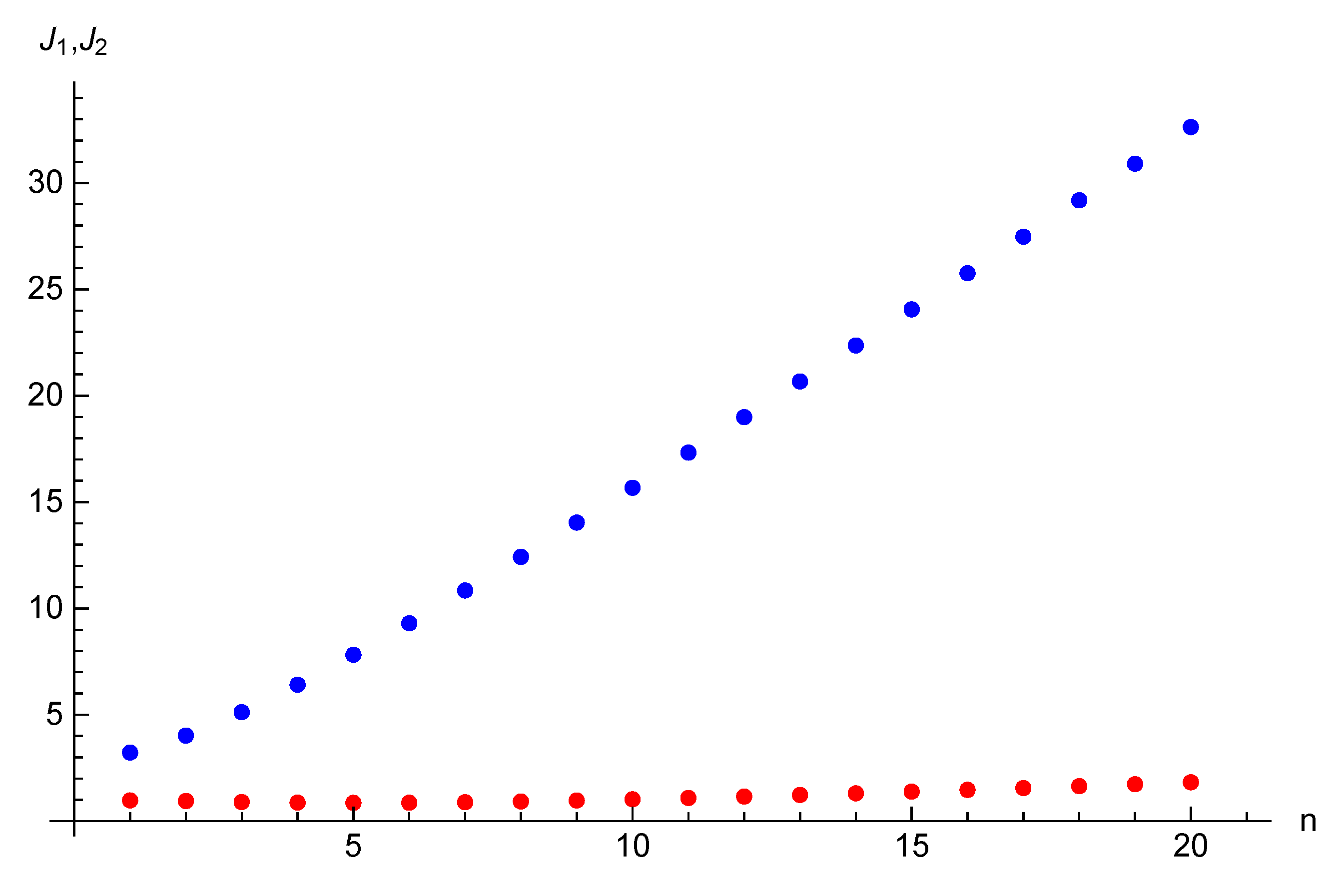
Example 3. Let the parameters of the game considered in this section be the following: , , and initial opinions be , . For time horizon , target opinions are , . The equilibrium state and strategy trajectories are presented on Figure 5 and Figure 6. The equilibrium costs of Players 1 and 2 are is and , respectively. Example 4. We also demonstrate how the costs of the players depend on the number of agents n. Consider the game with two players and the following parameters: , , and let initial opinions be , . For time horizon , target opinions are , . Corresponding graphs of the costs as the functions on n are depicted on Figure 7. One can notice that the cost function of Player 1 who influences directly on agent 1 is non-monotonic. First, it decreases for n from 1 to 5, then it increases. As this fact is not clearly recognized from Figure 7, we provide the values of the costs of Player 1 for periods from 1 to 20: 0.97, 0.94, 0.90, 0.87, 0.85, 0.86, 0.89, 0.92, 0.97, 1.03, 1.09, 1.16, 1.23, 1.31, 1.39, 1.47, 1.56, 1.64, 1.73, 1.83. The cost function of Player 2 is an increasing function of the number of agents in the network.
Remark 2. The Euler-equation approach can be considered as an indirect method of solving optimal control problems contrary to Pontryagin’s maximum principle. The Euler-equation approach defines the system of equations with respect to state variables. In many cases the method leads to a solution of difference equation with respect to state variables. We should notice the computational advantage of the Euler-equation, the realizations of which (see Examples 1–4) provide better results compared with realizations of Pontryagin’s maximum principle, e.g., the program finding the equilibrium strategies and costs in Example 2 for 20 periods provides the results on Euler-equation approach in 5 s, but on Pontryagin’s maximum principle, it takes more than 20 min.


