The Stability and Stabilization of Infinite Dimensional Caputo-Time Fractional Differential Linear Systems

Abstract

We investigate the stability and stabilization concepts for infinite dimensional time fractional differential linear systems in Hilbert spaces with Caputo derivatives. Firstly, based on a family of operators generated by strongly continuous semigroups and on a probability density function, we provide sufficient and necessary conditions for the exponential stability of the considered class of systems. Then, by assuming that the system dynamics are symmetric and uniformly elliptical and by using the properties of the Mittag–Leffler function, we provide sufficient conditions that ensure strong stability. Finally, we characterize an explicit feedback control that guarantees the strong stabilization of a controlled Caputo time fractional linear system through a decomposition approach. Some examples are presented that illustrate the effectiveness of our results.

1. Introduction

Fractional order calculus is a natural generalization of classical integer order calculus. It deals with integrals and derivatives of an arbitrary real or complex order. Fractional order calculus has become very popular in recent years, due to its demonstrated applications in many fields of applied sciences and engineering, such as the spread of contaminants in underground water, charge transport in amorphous semiconductors, and diffusion of pollution in the atmosphere [1,2,3]. Because it generalizes and includes in the limit the integer order calculus, fractional calculus has the potential to accomplish much more than what integer order calculus achieves [4]. In particular, it has proved to be a powerful tool to describe long-term memory and hereditary properties of various dynamical complex processes [5]; diffusion processes, such as those found in batteries [6]; and electrochemical and control processes [7], to model and control epidemics [8,9] and mechanical properties of viscoelastic systems and damping materials, such as stress and strain [10].

One can find in the literature several different fractional calculuses. Here we use the fractional calculus of Caputo, which was introduced by Michele Caputo in his 1967 paper [11]. Such calculus has appeared, in a natural way, for representing observed phenomena in laboratory experiments and field observations, where the mathematical theory was checked with experimental data. Indeed, the operator introduced by Caputo in 1967, and used by us in the present work, represents an observed linear dissipative mechanism phenomenon with a time derivative of order 0.15 entering the stress-strain relation [11]. More recently, a variational analysis with Caputo operators has been developed, which provides further mathematical substance to the use of Caputo fractional operators [12,13].

In the analysis and design of control systems, the stability issue always has an important role [14,15]. For a dynamical system, an equilibrium state is said to be stable if said system remains close to this state for small disturbances, and for an unstable system the question is how to stabilize it, especially by a feedback control law [16]. The stabilization concept for integer order systems and related problems has been considered in several works; see, e.g., [17,18,19,20] and references cited therein. In [17], the relationship between the asymptotic behavior of a system, the spectrum properties of its dynamics, and the existence of a Lyapunov functional is provided. Several techniques are considered to study different kinds of stabilization; for example, the exponential stabilization was studied via a decomposition method [19], and the strong stabilization was developed using the Riccati approach [20].

Similarly to classical dynamical systems, stability analysis is a central task in the study of fractional dynamical systems, which has attracted the increasing interest of many researchers [9,21]. For finite dimensional systems, the stability concept for fractional differential systems equipped with the Caputo derivative was investigated in many works [22]. In [23], Matignon studies the asymptotic behavior for linear fractional differential systems with the Caputo derivative, where their dynamics A are a constant coefficient matrix. In this case, the stability is guaranteed if the eigenvalues of the dynamics matrix A, $\lambda \in \sigma \left(A\right)$, satisfy $\left|arg\left(\lambda \right)\right|>{\displaystyle \frac{\pi \alpha }{2}}$ [23]. Since then, many scholars have carried out further studies on the stability for different classes of fractional linear systems [24,25]. In [24], stability theorems for fractional differential systems, which include linear systems, time-delayed systems, and perturbed systems, are established, while in [25], Ge, Chen, and Kou provide results on the Mittag–Leffler stability and propose a Lyapunov direct method, which covers the power law stability and the exponential stability. See also [26], where the Mittag–Leffler and the class-K function stability of fractional differential equations of order $\alpha \in (1,2)$ are investigated. In 2018, the notion of regional stability was introduced for fractional systems in [27], where the authors study the Mittag–Leffler stability and the stabilization of systems with Caputo derivatives, but only on a sub-region of its geometrical domain. More recently, fractional output stabilization problems for distributed systems in the Riemann–Liouville sense were studied [28,29,30], where feedback controls, which ensure exponential, strong, and weak stabilization of the state fractional spatial derivatives, with real and complex orders, are characterized.

An analysis of the literature shows that existing results on stability of fractional systems are essentially limited to finite-dimensional fractional order linear systems, while results on infinite-dimensional spaces are a rarity. In contrast, here we investigate global stability and stabilization of infinite dimensional fractional dynamical linear systems in the Hilbert space $L^2\left(\mathsf{\Omega }\right)$ with Caputo derivatives of fractional order $0<\alpha <1$. In particular, we characterize exponential and strong stability for fractional Caputo systems on infinite-dimensional spaces.

The remainder of this paper is organized as follows. In Section 2, some basic knowledge of fractional calculus and some preliminary results, which will be used throughout the paper, are given. In Section 3, we prove results on the global asymptotic and exponential stability of Caputo-time fractional differential linear systems. In contrast with available results in the literature, which are restricted to systems of integer order or to fractional systems in the finite dimensional state space ${\mathbb{R}}^n$, here we study a completely different class of systems: we investigate fractional linear systems where the state space is the Hillbert space $L^2\left(\mathsf{\Omega }\right)$. We also characterize the stabilization of a controlled Caputo diffusion linear system via a decomposition method. Section 4 presents the main conclusions of the work and some interesting open questions that deserve further investigations.

2. Preliminaries and Notation

In this section, we introduce several definitions and results of fractional calculus that are used in the sequel.

Definition 1

([2]). Let $0<\alpha <1$ and $T>0$. The Caputo derivative of fractional order α for an absolutely continuous function $y(·)$ on $[0,T]$ can be defined as follows:

$${}^C{D}_t^{\alpha }y\left(t\right)={\displaystyle \frac{1}{\mathsf{\Gamma }(1-\alpha )}}{\int }_0^t{(t-s)}^{-\alpha }{\displaystyle \frac{d}{ds}}y\left(s\right)\mathrm{d}s,$$

where $\mathsf{\Gamma }(1-\alpha )$ is the Euler Gamma function.

Lemma 1

([31]). For any given function $g\in L^2(0,T,L^2\left(\mathsf{\Omega }\right))$, we say that function $y\in C(0,T,L^2\left(\mathsf{\Omega }\right))$ is a mild solution of the system

$$\left\{\begin{array}{cc}{}^C{D}_t^{\alpha }y\left(t\right)=Ay\left(t\right)+g\left(t\right)\hfill & t\in ]0,+\infty [\hfill \\ y\left(0\right)=y_0\hfill & y_0\in L^2\left(\mathsf{\Omega }\right)\hfill \end{array}\right.$$

(1)

if it satisfies

$$y\left(t\right)=S_{\alpha }\left(t\right)y_0+{\int }_0^t{(t-s)}^{\alpha -1}{K}_{\alpha }(t-s)g\left(s\right)\mathrm{d}s,$$

(2)

where

$$S_{\alpha }\left(t\right)={\int }_0^{+\infty }{\mathsf{\Psi }}_{\alpha }\left(\theta \right)S\left(t^{\alpha }\theta \right)\mathrm{d}\theta$$

(3)

and

$$K_{\alpha }\left(t\right)=\alpha {\int }_0^{+\infty }\theta {\mathsf{\Psi }}_{\alpha }\left(\theta \right)S\left(t^{\alpha }\theta \right)\mathrm{d}\theta$$

(4)

with

$${\mathsf{\Psi }}_{\alpha }\left(\theta \right)=\frac{1}{\alpha }{\theta }^{-1-\frac{1}{\alpha }}{T}_{\alpha }\left({\theta }^{-\frac{1}{\alpha }}\right),$$

(5)

${\left(S\left(t\right)\right)}_{t\ge 0}$ the strongly continuous semigroup generated by operator A, and $T_{\alpha }$ the probability density function defined on $(0,\infty )$ by

$$T_{\alpha }=\frac{1}{\pi }\sum _{n=1}^{+\infty }{(-1)}^n{\theta }^{\alpha n-1}\frac{\mathsf{\Gamma }(n\alpha +1)}{n!}sin\left(n\pi \alpha \right).$$

Remark 1

([32]). The probability density function $T_{\alpha }$ defined on $(0,\infty )$ satisfies

$$T_{\alpha }\left(\theta \right)\ge 0,\hspace{1em}\theta \in (0,\infty ),\hspace{1em}\mathit{and}\hspace{1em}{\int }_0^{+\infty }{T}_{\alpha }\left(\theta \right)\mathrm{d}\theta =1.$$

Definition 2

([33]). The Mittag–Leffler function of one parameter is defined as

$$E_{\eta }\left(z\right)=\sum _{n=0}^{+\infty }\frac{z^n}{\mathsf{\Gamma }(\eta n+1)}\hspace{1em}\mathit{with}\hspace{1em}Re\left(\eta \right)>0,\hspace{1em}z\in \mathbb{C}.$$

Definition 3

([33]). The Mittag–Leffler function of two parameters is defined as

$$E_{\eta ,\beta }\left(z\right)=\sum _{n=0}^{+\infty }\frac{z^n}{\mathsf{\Gamma }(\eta n+\beta )}\hspace{1em}\mathit{with}\hspace{1em}Re\left(\eta \right)>0,\hspace{1em}\beta >0,\hspace{1em}z\in \mathbb{C}.$$

Remark 2.

The Mittag–Leffler function appears naturally in the solution of fractional differential equations and in various applications: see [33] and references therein. The exponential function is a special case of the Mittag–Leffler function [34]: for $\beta =1$ one has $E_{\eta ,1}\left(z\right)=E_{\eta }\left(z\right)$ and $E_{1,1}\left(z\right)=e^z$.

Lemma 2

([35]). The Mittag–Leffler function $E_{\alpha }(-t^{\alpha })$ is completely monotonic: for all $0<\alpha <1$, and for all $n\in \mathbb{N}$ and $t>0$, one has

$${(-1)}^n\frac{d^n}{d{t}^n}{E}_{\alpha }(-t^{\alpha })\ge 0.$$

Lemma 3

([36]). The generalized Mittag–Leffler function $E_{\eta ,\beta }(-x)$, $x\ge 0$, is completely monotonic for $\eta ,\beta >0$ if and only if $\eta \in (0,1]$ and $\beta \ge \eta$.

Lemma 4

([37]). Let $\beta >0$, $0<\eta <2$, and μ be an arbitrary real number such that $\frac{\pi \eta }{2}<\mu <min\{\pi ,\pi \eta \}$. Then, the following asymptotic expressions hold:

• If $\left|arg\right(z\left)\right|\le \mu$ and $\left|z\right|>0$, then

  $$|E_{\eta ,\beta }\left(z\right)|\le M_1{(1+|z\left|\right)}^{(1-\beta )/\eta }{e}^{Re(z^{\frac{1}{\eta }})}+\frac{M_2}{1+\left|z\right|};$$

  (6)
• If $\mu <\left|arg\right(z\left)\right|\le \pi$ and $\left|z\right|\ge 0$, then

  $$|E_{\eta ,\beta }\left(z\right)|\le \frac{M_2}{1+\left|z\right|},$$

  (7)

where $M_1$ and $M_2$ are positive constants.

3. Main Results

Our main goal is to study the stability and provide stabilization for a class of abstract Caputo-time fractional differential linear systems.

3.1. Stability of Time Fractional Differential Systems

Let $\mathsf{\Omega }$ be an open bounded subset of ${\mathbb{R}}^n$, $n=1,2,3,\dots$, and let us consider the following abstract time fractional order differential system:

$$\left\{\begin{array}{cc}{}^C{D}_t^{\alpha }z\left(t\right)=Az\left(t\right),\hfill & t\in ]0,+\infty [,\hfill \\ z\left(0\right)=z_0,\hfill & z_0\in L^2\left(\mathsf{\Omega }\right),\hfill \end{array}\right.$$

(8)

where ${}^C{D}_t^{\alpha }$ is the left-sided Caputo fractional derivative of order $0<\alpha <1$; the second order operator $A:D\left(A\right)\subset L^2\left(\mathsf{\Omega }\right)⟶L^2\left(\mathsf{\Omega }\right)$ is linear with a dense domain, is such that the coefficients do not depend on time t, and is also the infinitesimal generator of the $C_0$-semi-group ${\left(S\left(t\right)\right)}_{t\ge 0}$ on the Hilbert state space $L^2\left(\mathsf{\Omega }\right)$ endowed with its usual inner product $<·,·>$ and the corresponding norm $\parallel ·\parallel$. The unique mild solution of system (8) can be written, from Lemma 1, as

$$z\left(t\right)=S_{\alpha }\left(t\right)z_0,$$

where $S_{\alpha }\left(t\right)$ is defined by (3).

We begin by proving the following lemma, which will be used thereafter.

Lemma 5.

Let A be the infinitesimal generator of a $C_0$-semi-group ${\left(S\left(t\right)\right)}_{t\ge 0}$ on the Hilbert space $L^2\left(\mathsf{\Omega }\right)$. Assume that there exists a function $h(·)\in L^2(0,+\infty ;{\mathbb{R}}^{+})$ satisfying

$$\parallel S_{\alpha }(t+s)z\parallel \le h\left(t\right)\parallel S_{\alpha }\left(s\right)z\parallel ,\hspace{1em}\forall t,s\ge 0,\hspace{1em}\forall z\in L^2\left(\mathsf{\Omega }\right).$$

(9)

Then the operators ${\left(S_{\alpha }\left(t\right)\right)}_{t\ge 0}$ are uniformly bounded.

Proof. 

To prove that ${\left(S_{\alpha }\left(t\right)\right)}_{t\ge 0}$ are bounded, we have to show that

$$\forall z\in L^2\left(\mathsf{\Omega }\right)\underset{t\ge 0}{sup}\parallel S_{\alpha }\left(t\right)z\parallel <\infty .$$

(10)

By reductio ad absurdum, let us suppose that (10) does not hold, which means that there exists a sequence $(t_s+{\tau }_n)$, $t_s>0$ and ${\tau }_n⟶+\infty$, satisfying

$$\parallel S_{\alpha }(t_s+{\tau }_n)z\parallel ⟶+\infty as n⟶+\infty .$$

(11)

From relation

$${\displaystyle {\int }_0^{+\infty }\parallel S_{\alpha }(s+{\tau }_n){z\parallel }^2\mathrm{d}s={\int }_{{\tau }_n}^{+\infty }{\parallel S_{\alpha }\left(s\right)z\parallel }^2\mathrm{d}s, 0\le s<+\infty ,}$$

it follows that the right-hand side goes to 0 as $n⟶+\infty$. Using Fatou’s Lemma yields

$$\underset{n⟶+\infty }{lim inf} \parallel S_{\alpha }(s+{\tau }_n)z\parallel =0 \forall s>0.$$

Therefore, for some $s_0<t_s$, we may find a subsequence ${\tau }_{n_k}$ such that

$$\underset{k⟶+\infty }{lim}\parallel S_{\alpha }(s_0+{\tau }_{n_k})z\parallel =0.$$

By virtue of condition (9), one obtains

$$\parallel S_{\alpha }(t_s+{\tau }_{n_k})z\parallel \le h(t_s-s_0)\parallel S_{\alpha }(s_0+{\tau }_{n_k})z\parallel \underset{k⟶+\infty }{⟶0},$$

which contradicts (11). The intended conclusion follows from the uniform boundedness principle. □

Definition 4.

Let $z_0\in L^2\left(\mathsf{\Omega }\right)$. System (8) is said to be exponentially stable if there exist two strictly positive constants, $M>0$ and $\omega >0$, such that

$$\parallel z\left(t\right)\parallel \le M{e}^{-\omega t}\parallel z_0\parallel ,\hspace{1em}\forall t\ge 0.$$

The next theorem provides necessary and sufficient conditions for exponential stability of the abstract fractional order differential system (8).

Theorem 1.

Suppose that the operators ${\left(S_{\alpha }\left(t\right)\right)}_{t\ge 0}$ fulfill assumption (9) and

$$\forall z\in L^2\left(\mathsf{\Omega }\right)\hspace{1em}\parallel S_{\alpha }(t+s)z\parallel \le \parallel S_{\alpha }\left(t\right)z\parallel ·\parallel S_{\alpha }\left(s\right)z\parallel ,\hspace{1em}\forall t,s\ge 0.$$

(12)

Then, system (8) is exponentially stable if, and only if, for every $z\in L^2\left(\mathsf{\Omega }\right)$ there exists a positive constant $\delta <\infty$ such that

$${\displaystyle {\int }_0^{+\infty }{\parallel S_{\alpha }\left(t\right)z\parallel }^2\mathrm{d}t<\delta .}$$

(13)

Proof. 

One has

$$\begin{array}{cc}\hfill t\parallel S_{\alpha }{\left(t\right)z\parallel }^2& {\displaystyle ={\int }_0^t{\parallel S_{\alpha }\left(t\right)z\parallel }^2\mathrm{d}s}\hfill \\ & {\displaystyle ={\int }_0^t{\parallel S_{\alpha }(t-s+s)z\parallel }^2\mathrm{d}s.}\hfill \end{array}$$

Combining assumption (9), Lemma 5, and condition (13), one gets

$$\begin{array}{cc}\hfill t\parallel S_{\alpha }{\left(t\right)z\parallel }^2& {\displaystyle \le {\int }_0^t\parallel S_{\alpha }{\left(s\right)z\parallel }^2{\parallel S_{\alpha }(t-s)z\parallel }^2\mathrm{d}s}\hfill \\ & \le {N\delta \parallel z\parallel }^2\hfill \end{array}$$

for some $N>0$. Therefore, for t sufficiently large, it follows that

$$\parallel S_{\alpha }\left(t\right)\parallel <1.$$

Then, there exists $t_1>0$ such that

$$ln\parallel S_{\alpha }\left(t\right)\parallel <0,\hspace{1em}\forall t\ge t_1.$$

Thus,

$${\omega }_0=\underset{t\ge 0}{inf} {\displaystyle \frac{ln\parallel S_{\alpha }\left(t\right)\parallel }{t}}<0.$$

Now, let us show that

$${\omega }_0=\underset{t⟶+\infty }{lim}\frac{ln\parallel S_{\alpha }\left(t\right)\parallel }{t}.$$

(14)

Let $t_s>0$ be a fixed number and $N^{{}^{\prime }}={\displaystyle \underset{t\in [0,t_s]}{sup}}\parallel S_{\alpha }\left(t\right)\parallel$. Thus, for each $t>t_s$, there exists $m\in \mathbb{N}$ such that $m{t}_s\le t\le (m+1)t_s$. From (12), it follows that

$$\begin{array}{cc}\hfill \parallel S_{\alpha }\left(t\right)\parallel & =\parallel S_{\alpha }(m{t}_s+(t-m{t}_s))\parallel \hfill \\ & \le \parallel S_{\alpha }\left(m{t}_s\right)\parallel \parallel S_{\alpha }(t-m{t}_s)\parallel ,\hfill \end{array}$$

which yields

$$\frac{ln\parallel S_{\alpha }\left(t\right)\parallel }{t}\le \frac{ln\parallel S_{\alpha }\left(m{t}_s\right)\parallel }{t}+\frac{ln\parallel S_{\alpha }(t-m{t}_s)\parallel }{t}.$$

Using again (12), it results that

$$\frac{ln\parallel S_{\alpha }\left(t\right)\parallel }{t}\le \frac{m{t}_s}{t}\frac{ln\parallel S_{\alpha }\left(t_s\right)\parallel }{t_s}+\frac{ln\parallel N^{{}^{\prime }}\parallel }{t}.$$

Since ${\displaystyle \frac{m{t}_s}{t}}\le 1$ and $t_s$ is arbitrary, one obtains

$$\underset{t⟶+\infty }{lim sup} \frac{ln\parallel S_{\alpha }\left(t\right)\parallel }{t}\le \underset{t>0}{inf} \frac{ln\parallel S_{\alpha }\left(t\right)\parallel }{t}\le \underset{t⟶+\infty }{lim inf} \frac{ln\parallel S_{\alpha }\left(t\right)\parallel }{t}.$$

Consequently, (14) holds. Hence, we conclude that for all $\omega \in ]0,-{\omega }_0[$, there exists $M>0$ such that

$$\forall z\in L^2\left(\mathsf{\Omega }\right)\hspace{1em}\parallel S_{\alpha }\left(t\right)z\parallel \le M{e}^{-\omega t}\parallel z\parallel , \forall t\ge 0,$$

which means that system (8) is exponentially stable. The converse is obvious. □

Remark 3.

When $\alpha =1$, the conditions (9) and (12) are verified, and we retrieve from our Theorem 1 the results established in [17,18] about the exponential stability of system (8) on Ω, which is equivalent to

$${\int }_0^{+\infty }{\parallel S\left(t\right)z\parallel }^2\mathrm{d}t<\infty ,\hspace{1em}\forall z\in L^2\left(\mathsf{\Omega }\right).$$

Definition 5.

Let $z_0\in L^2\left(\mathsf{\Omega }\right)$. System (8) is said to be strongly stable if its corresponding solution $z\left(t\right)$ satisfies

$$\parallel z\left(t\right)\parallel ⟶0 as t⟶+\infty .$$

In our next theorem, we provide sufficient conditions that guaranty the strong stability of the fractional order differential system (8). The result generalizes the asymptotic result established by Matignon for finite dimensional state spaces, where the dynamics of the system A are considered to be a matrix with constant coefficients in ${\mathbb{R}}^n$ [23]. In contrast, here we tackle the stability for a different class of systems. Precisely, we consider fractional systems where the system dynamics A are a linear operator generating a strongly continuous semigroup in the infinite dimensional state space $L^2\left(\mathsf{\Omega }\right)$.

Theorem 2.

Let ${\left({\lambda }_p\right)}_{p\ge 1}$ and ${\left({\varphi }_p\right)}_{p\ge 1}$ be the eigenvalues and the corresponding eigenfunctions of operator A on $L^2\left(\mathsf{\Omega }\right)$. If A is a symmetric uniformly elliptical operator, then system (8) is strongly stable on Ω.

Proof. 

Since A is a symmetric uniformly elliptical operator, it follows that system (8) admits a weak solution defined by

$$z\left(t\right)=\sum _{p=1}^{+\infty }{E}_{\alpha }\left({\lambda }_p{t}^{\alpha }\right)\langle z_0,{\varphi }_p\rangle {\varphi }_p\hspace{1em}\forall z_0\in L^2\left(\mathsf{\Omega }\right),$$

where ${\left({\lambda }_p\right)}_{p\ge 1}$ satisfy

$$0>{\lambda }_1\ge {\lambda }_2\ge \cdots \ge {\lambda }_j\ge \cdots ,\underset{j⟶\infty }{lim}=-\infty ,$$

and ${\left({\varphi }_p\right)}_{p\ge 1}$ forms an orthonormal basis in $L^2\left(\mathsf{\Omega }\right)$ [38,39]. Using the fact that function $E_{\alpha }(-t^{\alpha })$ is completely monotonic, for all $\alpha \in (0,1)$ and $t>0$ (Lemma 2), yields

$$\begin{array}{cc}\hfill \parallel z\left(t\right)\parallel & =∥{\displaystyle \sum _{p=1}^{+\infty }{E}_{\alpha }\left({\lambda }_p{t}^{\alpha }\right)\langle z_0,{\varphi }_p\rangle {\varphi }_p}∥\hfill \\ & \le |E_{\alpha }\left({\lambda }_1{t}^{\alpha }\right)|\parallel z_0\parallel .\hfill \end{array}$$

Moreover, from Lemma 4, it follows that

$$\parallel z\left(t\right)\parallel \le \frac{M_2}{1-{\lambda }_1{t}^{\alpha }}\parallel z_0\parallel ⟶0\hspace{1em}\mathrm{as}\hspace{1em}t⟶+\infty$$

for some $M_2>0$. Hence, system (8) is strongly stable on $\mathsf{\Omega }$. □

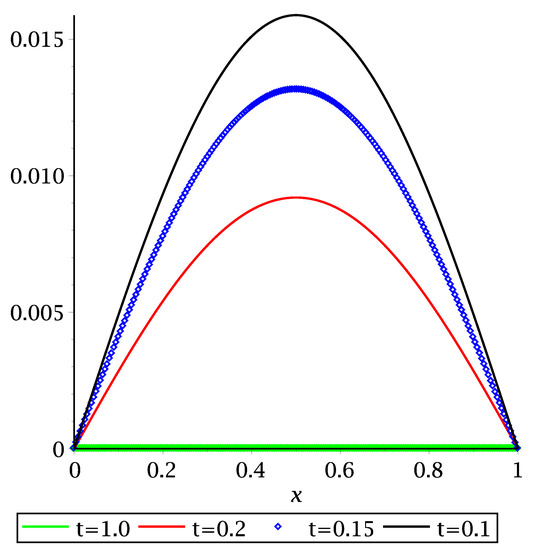
Example 1.

Let us consider, on $\mathsf{\Omega }=]0,1[$, the following one-dimensional fractional diffusion system defined by

$$\left\{\begin{array}{cc}{}^C{D}_t^{0.5}z(x,t)={\displaystyle \frac{{\partial }^{2}z}{\partial x^2}}(x,t),\hfill & x\in \mathsf{\Omega },\hspace{1em}t\in ]0,+\infty [,\hfill \\ z(0,t)=z(1,t)=0,\hfill & \forall t>0,\hfill \\ z(x,0)=z_0,\hfill & x\in \mathsf{\Omega },\hfill \end{array}\right.$$

(15)

where the second order operator $A={\displaystyle \frac{{\partial }^2}{\partial x^2}}$ has its spectrum given by the eigenvalues ${\lambda }_p=-{\left(p\pi \right)}^2$, $p\ge 1$, and the corresponding eigenfunctions are ${\varphi }_p\left(x\right)=\sqrt{\frac{2}{1+{\left(p\pi \right)}^2}}sin\left(p\pi x\right)$, $p\ge 1$. Operator A generates a $C_0$-semi-group ${\left(S\left(t\right)\right)}_{t\ge 0}$ defined by

$$S\left(t\right)z_0=\sum _{p=1}^{+\infty }{e}^{{\lambda }_{p}t}\langle z_0,{\varphi }_p\rangle {\varphi }_p.$$

Moreover, the solution of system (15) is given by

$$S_{0.5}\left(t\right)z_0=\sum _{p=1}^{+\infty }{E}_{0.5}\left({\lambda }_p{t}^{0.5}\right)\langle z_0,{\varphi }_p\rangle {\varphi }_p.$$

One has that operator A is symmetric and uniformly elliptical. Consequently, from our Theorem 2, we deduce that system (15) is strongly stable on Ω. This is illustrated numerically in Figure 1 for $z(x,0)=sin\left(\pi x\right)$, $t=0.1$, $t=0.15$, $t=0.2$, and $t=1.0$.

3.2. Stabilization of Time Fractional Differential Systems

Let $\mathsf{\Omega }$ be an open bounded subset of ${\mathbb{R}}^n$, $n=1,2,3,\dots$ We consider the following Caputo-time fractional differential linear system:

$$\left\{\begin{array}{cc}{}^C{D}_t^{\alpha }z\left(t\right)=Az\left(t\right)+Bu\left(t\right),\hfill & t\in ]0,+\infty [,\hspace{1em}0<\alpha <1,\hfill \\ z\left(0\right)=z_0,\hfill & z_0\in L^2\left(\mathsf{\Omega }\right),\hfill \end{array}\right.$$

(16)

with the same assumptions on A as in Section 3.1 and where B is a bounded linear operator from U into $L^2\left(\mathsf{\Omega }\right)$, where U is the space of controls, assumed to be a Hilbert space. By Lemma 1, the unique mild solution $z(·)$ of system (16) is defined by

$${\displaystyle z\left(t\right)=S_{\alpha }\left(t\right)z_0+{\int }_0^t{(t-s)}^{\alpha -1}{K}_{\alpha }(t-s)Bu\left(s\right)\mathrm{d}s,}$$

(17)

where $S_{\alpha }\left(t\right)$ and $K_{\alpha }\left(t\right)$ are given, respectively, by (3) and (4).

Definition 6.

System (16) is said to be exponentially (respectively strongly) stabilizable if there exists a bounded operator $K\in \mathcal{L}(L^2\left(\mathsf{\Omega }\right),U)$ such that the system

$$\left\{\begin{array}{cc}{}^C{D}_t^{\alpha }z\left(t\right)=(A+BK)z\left(t\right),\hfill & t\in ]0,+\infty [,\hfill \\ z\left(0\right)=z_0,\hfill & z_0\in L^2\left(\mathsf{\Omega }\right),\hfill \end{array}\right.$$

(18)

is exponentially (respectively strongly) stable on Ω.

Remark 4.

It is clear that the exponential stabilization of system (16) implies the strong stabilization of (16). Note that the concept is general: when $\alpha =1$, we obtain the classical definitions of stability and stabilization.

Let ${\left(S^k\left(t\right)\right)}_{t\ge 0}$ be the strongly continuous semi-group generated by $A+BK$, where $K\in \mathcal{L}(L^2\left(\mathsf{\Omega }\right),U)$ is the feedback operator. The unique mild solution of system (16) can be written as

$$z\left(t\right)=S_{\alpha }^k\left(t\right)z_0$$

with

$${\displaystyle S_{\alpha }^k\left(t\right)={\int }_0^{+\infty }{\mathsf{\Psi }}_{\alpha }\left(\theta \right)S^k\left(t^{\alpha }\theta \right)\mathrm{d}\theta ,}$$

where ${\mathsf{\Psi }}_{\alpha }\left(\theta \right)$ is defined by (5).

Theorem 3.

Let $A+BK$ generate a strongly continuous semi-group ${\left(S^k\left(t\right)\right)}_{t\ge 0}$ on $L^2\left(\mathsf{\Omega }\right)$. If the operator ${\left(S_{\alpha }^k\left(t\right)\right)}_{t\ge 0}$ satisfies conditions (9) and (12) and if

$${\displaystyle \forall z\in L^2\left(\mathsf{\Omega }\right)\hspace{1em}{\int }_0^{+\infty }{\parallel S_{\alpha }^k\left(t\right)z\parallel }^2\mathrm{d}t< \infty }$$

holds, then system (16) is exponentially stabilizable on Ω.

Proof. 

The proof is similar to the proof of Theorem 1. □

Theorem 4.

Let ${\left({\lambda }_p^k\right)}_{p\ge 1}$ and ${\left({\varphi }_p^k\right)}_{p\ge 1}$ be the eigenvalues and the corresponding eigenfunctions of operator $A+BK$ on $L^2\left(\mathsf{\Omega }\right)$. If $A+BK$ is a symmetric uniformly elliptical operator, then system (16) is strongly stabilizable on Ω.

Proof. 

The proof is similar to the proof of Theorem 2. □

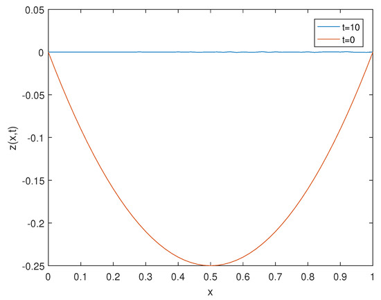
Example 2.

Let us consider, on $\mathsf{\Omega }=]0,1[$, the following fractional differential system of order $\alpha =0.2$:

$$\left\{\begin{array}{cc}{\displaystyle {}^C{D}_t^{0.2}z(x,t)=\frac{1}{100}{\displaystyle \frac{{\partial }^{2}z}{\partial x^2}}(x,t)+\frac{1}{2}z(x,t)+BKz(x,t),}\hfill & (x,t)\in \mathsf{\Omega }\times ]0,+\infty [,\hfill \\ z(0,t)=z(1,t)=0,\hfill & \forall t>0,\hfill \\ z(x,0)=z_0,\hfill & x\in \mathsf{\Omega },\hfill \end{array}\right.$$

(19)

with the linear bounded operator $B=I$ and where we take $K=-B^{*}=-I$. The operator

$$A+BK=\frac{1}{100}{\displaystyle \frac{{\partial }^2}{\partial x^2}}-\frac{1}{2},$$

with spectrum given by the eigenvalues ${\lambda }_p^k=-\frac{1}{2}-\frac{1}{100}{\left(p\pi \right)}^2$, $p\ge 1$, and the corresponding eigenfunctions ${\varphi }_p^k\left(x\right)=\sqrt{\frac{2}{1+{\left(p\pi \right)}^2}}cos\left(p\pi x\right)$, $p\ge 1$, generates a $C_0$-semi-group ${\left(S^k\left(t\right)\right)}_{t\ge 0}$ defined by

$${\displaystyle S^k\left(t\right)z_0=\sum _{p=1}^{+\infty }{e}^{{\lambda }_p^{k}t}\langle z_0,{\varphi }_p^k\rangle {\varphi }_p^k.}$$

Furthermore, the solution of system (19) can be written as

$${\displaystyle z\left(t\right)=S_{0.2}^k\left(t\right)z_0=\sum _{p=1}^{+\infty }{E}_{0.2}\left({\lambda }_p^k{t}^{0.2}\right)\langle z_0,{\varphi }_p^k\rangle {\varphi }_p^k.}$$

It is clear that $A+BK$ is a symmetric and uniformly elliptical operator. Hence, from Theorem 4, we deduce that system (19) is strongly stabilizable on Ω, i.e., the system

$$\left\{\begin{array}{cc}{\displaystyle {}^C{D}_t^{0.2}z(x,t)=\frac{1}{100}{\displaystyle \frac{{\partial }^{2}z}{\partial x^2}}(x,t)+\frac{1}{2}z(x,t)+Bu\left(t\right),}\hfill & (x,t)\in \mathsf{\Omega }\times ]0,+\infty [,\hfill \\ z(0,t)=z(1,t)=0,\hfill & \forall t>0,\hfill \\ z(x,0)=z_0,\hfill & x\in \mathsf{\Omega },\hfill \end{array}\right.$$

is strongly stabilizable by the feedback control $u\left(t\right)=-B^{*}z\left(t\right)$. Figure 2 shows, for $z(x,0)=x(x-1)$, that the state $z(x,t)$ of system (19) is unstable at $t=0$. Moreover, we see that the state evolves close to 0 at $t=10$. Numerically, the state is stabilized by $u\left(t\right)=-B^{*}z\left(t\right)$ with an error equal to $1.75\times {10}^{-04}$.

3.3. Decomposition Method

Now, we study the stabilization of system (16) using the decomposition method, which consists of decomposing the state space and the system using the spectral properties of operator A.

Let $\xi >0$ be fixed and assume that there are at most finitely-many nonnegative eigenvalues of A, each with finite-dimensional eigenspace. In other words, assume there exists $l\in \mathbb{N}$ such that

$$\sigma \left(A\right)={\sigma }_u\left(A\right)\cup {\sigma }_s\left(A\right),$$

(20)

where ${\sigma }_u\left(A\right)=\sigma \left(A\right)\cap \{{\lambda }_p, p=1,2,\dots ,l\}$, ${\sigma }_s\left(A\right)=\sigma \left(A\right)\cap \{{\lambda }_p, p=l+1,l+2\dots \}$ with ${\lambda }_l\ge 0$ and ${\lambda }_{l+1}\le -\xi$. Because the sequence ${\left({\varphi }_p\right)}_{p\ge 1}$ forms a complete and orthonormal basis in $H=L^2\left(\mathsf{\Omega }\right)$, it follows that the state space H can be decomposed as

$$H=H_u\oplus H_s,$$

(21)

where $H_u=PH=\mathrm{span}\{{\varphi }_1,{\varphi }_2,\dots ,{\varphi }_l\}$ and $H_s=(I-P)H=\mathrm{span}\{{\varphi }_{l+1},{\varphi }_{l+2},\dots \}$ with $P\in \mathcal{L}\left(H\right)$ the projection operator [40]. Hence, system (16) can be decomposed into the following two sub-systems:

$$\left\{\begin{array}{c}{}^C{D}_t^{\alpha }{z}_u\left(t\right)=A_u{z}_u\left(t\right)+PBu\left(t\right),\hfill \\ z_{0u}=P{z}_0,\hfill \end{array}\right.$$

(22)

and

$$\left\{\begin{array}{c}{}^C{D}_t^{\alpha }{z}_s\left(t\right)=A_s{z}_s\left(t\right)+(I-P)Bu\left(t\right),\hfill \\ z_{0s}=(I-P)z_0,\hfill \end{array}\right.$$

(23)

where $A_s$ and $A_u$ are the restrictions of A on $H_s$ and $H_u$, respectively, and are such that $\sigma \left(A_s\right)={\sigma }_s\left(A\right)$, $\sigma \left(A_u\right)={\sigma }_u\left(A\right)$, and $A_u$ is a bounded operator on $H_u$.

Our next result asserts that stabilization of system (16) is equivalent to the one of system (22).

Theorem 5.

Let the spectrum $\sigma \left(A\right)$ of A satisfy the above spectrum decomposition assumptions (20) for some $\xi >0$ and $A_s$ be a symmetric uniformly elliptical operator. If system (22) is strongly stabilizable by the control

$$u\left(t\right)=D_u{z}_u\left(t\right)$$

(24)

with $D_u\in \mathcal{L}(H,U)$ such that

$$\parallel z_u\left(t\right)\parallel \le C t^{-\mu },\hspace{1em}\mu ,C>0,$$

(25)

then system (16) is strongly stabilizable using the feedback control $v\left(t\right)=D_u{z}_u\left(t\right)$.

Proof. 

Using the fact that system (22) is strongly stabilizable by control (24), and inequality (25) yields

$$\parallel z_u\left(t\right)\parallel ⟶0 \mathrm{as} t⟶+\infty$$

(26)

and

$$\parallel u\left(t\right)\parallel \le C\parallel D_u\parallel t^{-\mu },$$

(27)

the unique weak solution of system (23) can be written in the space $H_s$ as

$${\displaystyle z_s\left(t\right)=\sum _{p=l+1}^{+\infty }{E}_{\alpha }\left({\lambda }_p{t}^{\alpha }\right)\langle z_{0s},{\varphi }_p\rangle {\varphi }_p+\sum _{p=l+1}^{+\infty }{\int }_0^t{(t-s)}^{\alpha -1}{E}_{\alpha ,\alpha }\left({\lambda }_p{(t-s)}^{\alpha }\right)\langle (I-P)Bu\left(s\right),{\varphi }_p\rangle {\varphi }_p\mathrm{d}s}$$

since $A_s$ is a symmetric uniformly elliptical operator [38]. Using the spectrum decomposition relation (20), Lemma 2, and Lemma 3, one has that

$$E_{\alpha }\left({\lambda }_p{t}^{\alpha }\right)\le E_{\alpha }(-\xi t^{\alpha })\hspace{1em}\mathrm{for} \mathrm{all} p\ge l+1$$

(28)

and

$$E_{\alpha ,\alpha }\left({\lambda }_p{(t-s)}^{\alpha }\right)\le E_{\alpha ,\alpha }(-\xi {(t-s)}^{\alpha })\hspace{1em}\mathrm{for} \mathrm{all} p\ge l+1.$$

(29)

Then, feeding system (23) by the same control $u\left(t\right)=D_u{z}_u\left(t\right)$ and using (27)–(29), it follows that

$$\begin{array}{cc}\hfill \parallel z_s\left(t\right)\parallel & {\displaystyle \le E_{\alpha }(-\xi t^{\alpha })\parallel z_{0s}\parallel +C\parallel D_u\parallel \parallel I-P\parallel \parallel B\parallel {\int }_0^t{(t-s)}^{\alpha -1}{s}^{-\mu }{E}_{\alpha ,\alpha }(-\xi {(t-s)}^{\alpha })\mathrm{d}s}\hfill \\ & {\displaystyle \le E_{\alpha }(-\xi t^{\alpha })\parallel z_{0s}\parallel +C\parallel D_u\parallel \parallel I-P\parallel \parallel B\parallel \sum _{n=1}^{+\infty }{\int }_0^t{\displaystyle \frac{{(-\xi )}^n{(t-s)}^{\alpha n+\alpha -1}{s}^{-\mu }\mathrm{d}s}{\mathsf{\Gamma }(\alpha n+\alpha )}}}\hfill \\ & {\displaystyle \le E_{\alpha }(-\xi t^{\alpha })\parallel z_{0s}\parallel +C\parallel D_u\parallel \parallel I-P\parallel \parallel B\parallel \sum _{n=1}^{+\infty }{\displaystyle \frac{{(-\xi )}^n{t}^{\alpha n+\alpha -\mu }}{\mathsf{\Gamma }(\alpha n+\alpha -\mu -1)\mathsf{\Gamma }{(1-\mu )}^{-1}}}}\hfill \\ & \le E_{\alpha }(-\xi t^{\alpha })\parallel z_{0s}\parallel +C\mathsf{\Gamma }(1-\mu )\parallel D_u\parallel \parallel I-P\parallel \parallel B\parallel t^{\alpha -\mu }{E}_{\alpha ,\alpha -\mu +1}(-\xi t^{\alpha }).\hfill \end{array}$$

Lemma 4 implies that

$$\parallel z_s\left(t\right)\parallel \le \frac{M_1}{1+\xi t^{\alpha }}\parallel z_{s0}\parallel +C\mathsf{\Gamma }(1-\mu )\parallel D_u\parallel \parallel I-P\parallel \parallel B\parallel \frac{M_2{t}^{\alpha -\mu }}{1+\xi t^{\alpha }}$$

for some $M_1,M_2>0$. Therefore,

$$\parallel z_s\left(t\right)\parallel ⟶0 \mathrm{as} t⟶+\infty .$$

(30)

On the other hand, we have that

$$\parallel z\left(t\right)\parallel =\parallel z_s\left(t\right)+z_u\left(t\right)\parallel \le \parallel z_s\left(t\right)\parallel +\parallel z_u\left(t\right)\parallel .$$

(31)

Combining (26), (30), and (31), we deduce the strong stabilization of system (16). □

4. Conclusions and Future Work

We investigated the stability problem of infinite dimensional time fractional differential linear systems under Caputo derivatives of order $\alpha \in (0,1)$, where the state space is the Hillbert space $L^2\left(\mathsf{\Omega }\right)$. We proved necessary and sufficient conditions for exponential stability and obtained a characterization for the asymptotic stability, which is guaranteed if the system dynamics are symmetric and uniformly elliptical. Moreover, some stabilization criteria were also proved. Finally, we investigated the strong stabilization of the system via a decomposition method; an explicit feedback control was obtained. Illustrative examples were given, showing the effectiveness of the theoretical results. As future work, we intend to extend our work to the class of infinite dimensional time fractional differential nonlinear systems. Various other questions are still open and deserve further investigations, such as studying boundary stability and gradient stability for time fractional differential linear systems or considering the more recent notion of $\mathsf{\Lambda }$-fractional derivative [41], and thus obtaining a geometrical interpretation.

References

- Rahimy, M. Applications of fractional differential equations. Appl. Math. Sci. (Ruse) 2010, 4, 2453–2461. [Google Scholar]
- Kilbas, A.A.; Srivastava, H.M.; Trujillo, J.J. THeory and Applications of Fractional Differential Equations; Elsevier Science B.V.: Amsterdam, The Netherlands, 2006. [Google Scholar]
- Diethelm, K. The Analysis of Fractional Differential Equations; Lecture Notes in Mathematics; Springer: Berlin, Germany, 2010; Volume 2004. [Google Scholar] [CrossRef]
- Hilfer, R. Applications of Fractional Calculus in Physics; World Scientific Publishing Co., Inc.: River Edge, NJ, USA, 2000. [Google Scholar] [CrossRef]
- Sabatier, J.; Agrawal, O.P.; Machado, J.A.T. Advances in Fractional Calculus; Springer: Dordrecht, The Netherlands, 2007. [Google Scholar] [CrossRef]
- Gabano, J.D.; Poinot, T. Fractional modelling and identification of thermal systems. Signal Process. 2011, 91, 531–541. [Google Scholar] [CrossRef]
- Ichise, M.; Nagayanagi, Y.; Kojima, T. An analog simulation of non-integer order transfer functions for analysis of electrode processes. J. Electroanal. Chem. Interfacial Electrochem. 1971, 33, 253–265. [Google Scholar] [CrossRef]
- Rosa, S.; Torres, D.F.M. Optimal control and sensitivity analysis of a fractional order TB model. Stat. Optim. Inf. Comput. 2019, 7, 617–625. [Google Scholar] [CrossRef]
- Silva, C.J.; Torres, D.F.M. Stability of a fractional HIV/AIDS model. Math. Comput. Simul. 2019, 164, 180–190. [Google Scholar] [CrossRef]
- Bagley, R.L.; Calico, R.A. Fractional order state equations for the control of viscoelastically damped structures. J. Guid. Control Dyn. 1991, 14, 304–311. [Google Scholar] [CrossRef]
- Caputo, M. Linear models of dissipation whose Q is almost frequency independent II. Fract. Calc. Appl. Anal. 2008, 11, 4–14, Reprinted from Geophys. J. R. Astr. Soc. 1967, 13, 529–539. [Google Scholar] [CrossRef]
- Malinowska, A.B.; Torres, D.F.M. Introduction to the Fractional Calculus of Variations; Imperial College Press: London, UK, 2012. [Google Scholar] [CrossRef]
- Almeida, R.; Pooseh, S.; Torres, D.F.M. Computational Methods in the Fractional Calculus of Variations; Imperial College Press: London, UK, 2015. [Google Scholar] [CrossRef]
- Mahmoud, M.S.; Karaki, B.J. Improved stability analysis and control design of reset systems. IET Control Theory Appl. 2018, 12, 2328–2336. [Google Scholar] [CrossRef]
- Rocha, D.; Silva, C.J.; Torres, D.F.M. Stability and optimal control of a delayed HIV model. Math. Methods Appl. Sci. 2018, 41, 2251–2260. [Google Scholar] [CrossRef]
- Sontag, E.D. Stability and feedback stabilization. In Mathematics of Complexity and Dynamical Systems; Springer: New York, NY, USA, 2012; Volumes 1–3, pp. 1639–1652. [Google Scholar] [CrossRef]
- Pritchard, A.J.; Zabczyk, J. Stability and stabilizability of infinite-dimensional systems. SIAM Rev. 1981, 23, 25–52. [Google Scholar] [CrossRef]
- Curtain, R.F.; Zwart, H. An Introduction to Infinite-Dimensional Linear Systems Theory; Texts in Applied Mathematics; Springer: New York, NY, USA, 1995; Volume 21. [Google Scholar] [CrossRef]
- Triggiani, R. On the stabilizability problem in Banach space. J. Math. Anal. Appl. 1975, 52, 383–403. [Google Scholar] [CrossRef]
- Balakrishnan, A.V. Strong stabilizability and the steady state Riccati equation. Appl. Math. Optim. 1981, 7, 335–345. [Google Scholar] [CrossRef]
- Wojtak, W.; Silva, C.J.; Torres, D.F.M. Uniform asymptotic stability of a fractional tuberculosis model. Math. Model. Nat. Phenom. 2018, 13, 9. [Google Scholar] [CrossRef]
- Zhang, F.; Li, C.; Chen, Y. Asymptotical stability of nonlinear fractional differential system with Caputo derivative. Int. J. Differ. Equ. 2011, 2011, 635165. [Google Scholar] [CrossRef]
- Matignon, D. Stability Results for Fractional Differential Equations with Applications to Control Processing; Computational Engineering in Systems Applications: Lille, France, 1996; Volume 2, pp. 963–968. [Google Scholar]
- Qian, D.; Li, C.; Agarwal, R.P.; Wong, P.J.Y. Stability analysis of fractional differential system with Riemann-Liouville derivative. Math. Comput. Modelling 2010, 52, 862–874. [Google Scholar] [CrossRef]
- Li, Y.; Chen, Y.; Podlubny, I. Stability of fractional-order nonlinear dynamic systems: Lyapunov direct method and generalized Mittag-Leffler stability. Comput. Math. Appl. 2010, 59, 1810–1821. [Google Scholar] [CrossRef]
- Matar, M.M.; Abu Skhail, E.S. On stability of nonautonomous perturbed semilinear fractional differential systems of order α∈(1, 2). J. Math. 2018, 2018, 1723481. [Google Scholar] [CrossRef]
- Ge, F.; Chen, Y.; Kou, C. Regional Analysis of Time-Fractional Diffusion Processes; Springer: Cham, Switzerland, 2018. [Google Scholar] [CrossRef]
- Zitane, H.; Larhrissi, R.; Boutoulout, A. On the fractional output stabilization for a class of infinite dimensional linear systems. In Recent Advances in Modeling, Analysis and Systems Control: Theoretical Aspects and Applications; Springer: Cham, Switzerland, 2020; pp. 241–259. [Google Scholar]
- Zitane, H.; Larhrissi, R.; Boutoulout, A. Fractional output stabilization for a class of bilinear distributed systems. Rend. Circ. Mat. Palermo 2019, 2, 1–16. [Google Scholar] [CrossRef]
- Zitane, H.; Larhrissi, R.; Boutoulout, A. Riemann Liouville fractional spatial derivative stabilization of bilinear distributed systems. J. Appl. Nonlinear Dyn. 2019, 8, 447–461. [Google Scholar] [CrossRef]
- Zhou, Y.; Jiao, F. Existence of mild solutions for fractional neutral evolution equations. Comput. Math. Appl. 2010, 59, 1063–1077. [Google Scholar] [CrossRef]
- Mainardi, F.; Paradisi, P.; Gorenflo, R. Probability distributions generated by fractional diffusion equations. arXiv 2007, arXiv:0704.0320. [Google Scholar]
- Erdélyi, A.; Magnus, W.; Oberhettinger, F.; Tricomi, F.G. Higher Transcendental Functions; Robert, E., Ed.; Krieger Publishing Co., Inc.: Melbourne, Australia, 1981; Volume III. [Google Scholar]
- Joshi, S.; Mittal, E.; Pandey, R.M. On Euler type integrals involving extended Mittag-Leffler functions. Bol. Soc. Parana. Mat. 2020, 38, 125–134. [Google Scholar]
- Mainardi, F. On some properties of the Mittag-Leffler function Eα(−tα), completely monotone for t > 0 with 0 < α < 1. Discrete Contin. Dyn. Syst. Ser. B 2014, 19, 2267–2278. [Google Scholar] [CrossRef]
- Schneider, W.R. Completely monotone generalized Mittag-Leffler functions. Exposition. Math. 1996, 14, 3–16. [Google Scholar]
- Podlubny, I. Fractional Differential Equations; Academic Press, Inc.: San Diego, CA, USA, 1999. [Google Scholar]
- Sakamoto, K.; Yamamoto, M. Initial value/boundary value problems for fractional diffusion-wave equations and applications to some inverse problems. J. Math. Anal. Appl. 2011, 382, 426–447. [Google Scholar] [CrossRef]
- Courant, R.; Hilbert, D. Methods of Mathematical Physics; Interscience Publishers, Inc.: New York, NY, USA, 1953; Volume I. [Google Scholar]
- Kato, T. Perturbation Theory for Linear Operators; Springer: New York, NY, USA, 1966. [Google Scholar]
- Lazopoulos, K.A.; Lazopoulos, A.K. On the Mathematical Formulation of Fractional Derivatives. Progr. Fract. Differ. Appl. 2019, 5, 261–267. [Google Scholar] [CrossRef]
© 2020 by the authors. Licensee MDPI, Basel, Switzerland. This article is an open access article distributed under the terms and conditions of the Creative Commons Attribution (CC BY) license (http://creativecommons.org/licenses/by/4.0/).