A Practical Traffic Assignment Model for Multimodal Transport System Considering Low-Mobility Groups


Abstract
1. Introduction
- (a)
- Unlike existing references, the generalized travel cost of a path is calculated by summing the travel costs of all links and intersections present in a path. Furthermore, the intersection can be classified into signalized and unsignalized, and, therefore, two different computing methods to calculate the travel time of an intersection in each trip mode are proposed.
- (b)
- In the private car mode, a traveler may choose a path with a longer travel time compared to the other paths because the fuel cost involved in travelling the path is the lowest. Hence, the link travel cost of a private car is calculated by a subjective weighting of the travel time and fuel cost. On the contrary, the walking and non-vehicle modes only consider the travel time because they are pollution-free and do not involve any fuel costs.
- (c)
- The existing time cost functions only consider the link impedance related to traffic flows rather than the actual situations. In this paper, the influence of traffic barricades present between different lanes is considered in the calculation of link travel costs of different trip modes. To effectively show the significance of this influence, we do not consider the traffic barricades present in the vehicle lanes because that only involves a single mode. The influence considered has implications in the following cases: (1) If there are no traffic barricades present between walking and non-vehicle lanes, the travel time of the former type of lanes can increase, and (2) if there are no traffic barricades between vehicle and non-vehicle lanes, the travel times of walking, non-vehicle, and private car can all increase.
- (a)
- (b)
- Improving the practicality of generalized travel costs, considering the travel times of both links and signalized and unsignalized intersections, the travel times and fuel costs of private cars, and the influence of traffic barricades present between different lanes in a path.
- (c)
- Using the MSWA to solve the proposed multimodal traffic assignment problem. To verify the model and the algorithm, a real case study is performed. Furthermore, the sensitivity of adjustment parameters related to travel costs is analyzed, the practicality of the proposed model is explored, and the results of traffic assignments obtained for different low-mobility groups are discussed.
2. Model Development
2.1. Equilibrium Analysis
2.2. Equivalent Transformation
3. Travel Cost Function of Different Trip Modes
- (a)
- travel times to traverse links and intersections in a path;
- (b)
- travel times and fuel costs of private cars;
- (c)
- the influence of traffic barricades between different lanes.
3.1. Private Car
3.2. Non-Vehicle
3.3. Walking
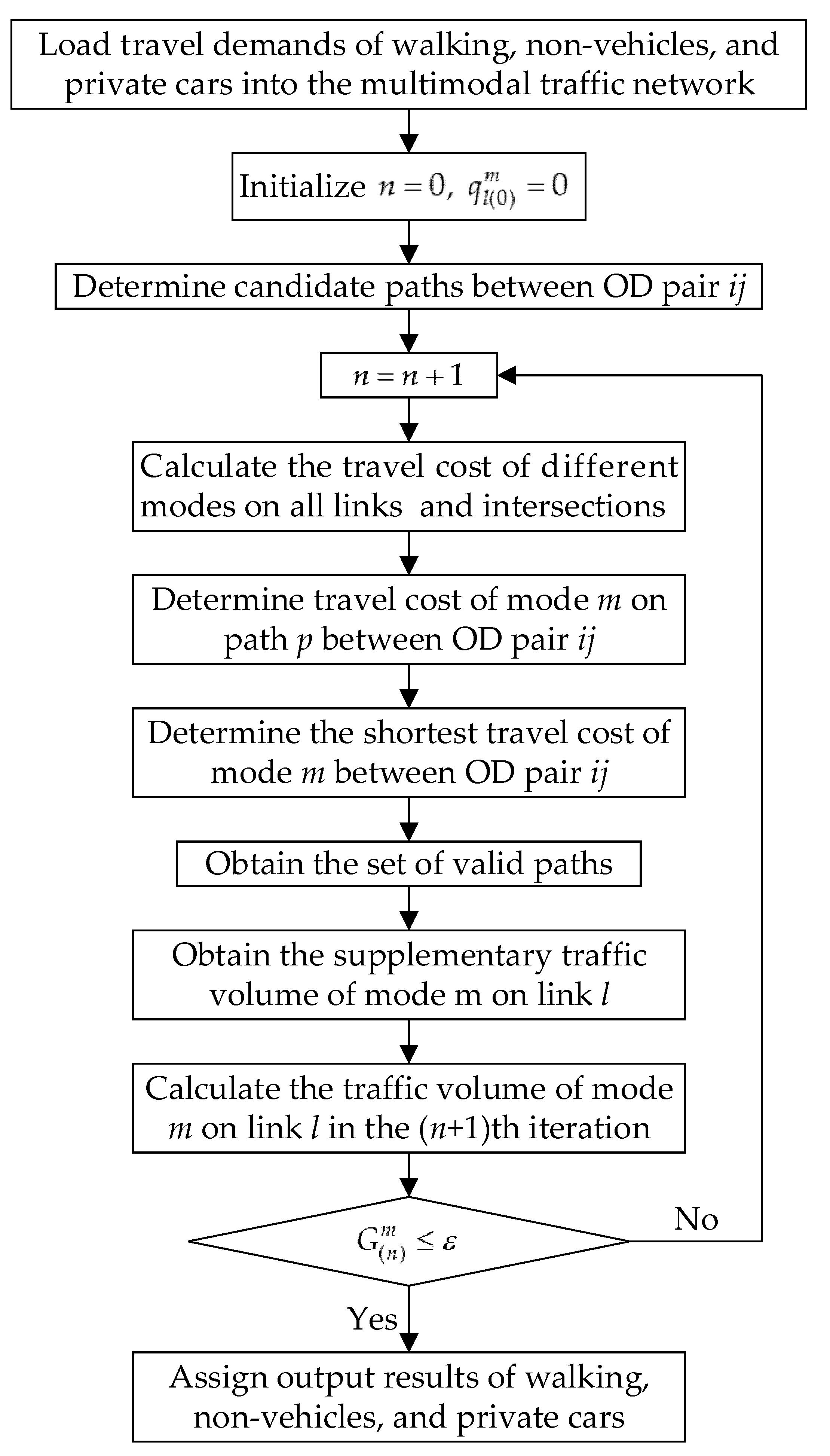
4. Proposed Solution
- Load the travel demands of walking, non-vehicle, and private cars into the multimodal traffic network.
- Initialize the iterations to n = 0, and the traffic volume of mode m on link l in the zeroth iteration to = 0.
- Determine different candidate paths between the O-D pair ij using the k-shortest path algorithm.
- In the nth iteration, calculate the travel cost of mode m on all links and intersections based on Equations (13), (16), (17), (19), (21), (22), (24), (27) and (28).
- In the nth iteration, determine the travel cost of mode m on candidate path p between the O-D pair ij using Equation (10) and select the shortest path travel cost of mode m between the O-D pair ij from among the different candidate paths.
- In the nth iteration, select valid paths from the candidate paths based on the decision condition, given by the following equation:where is the decision coefficient.
- In the nth iteration, assign travel demands of mode m into valid paths based on Equation (1), and obtain the supplementary traffic volume of mode m on link l.
- In the (n+1)th iteration, calculate the traffic volume of mode m on link l using (31).
- Check for convergence by calculating the error value of mode m in the nth iteration using Equation (32). Note that , where is the error parameter and is the equilibrium solution of mode m.
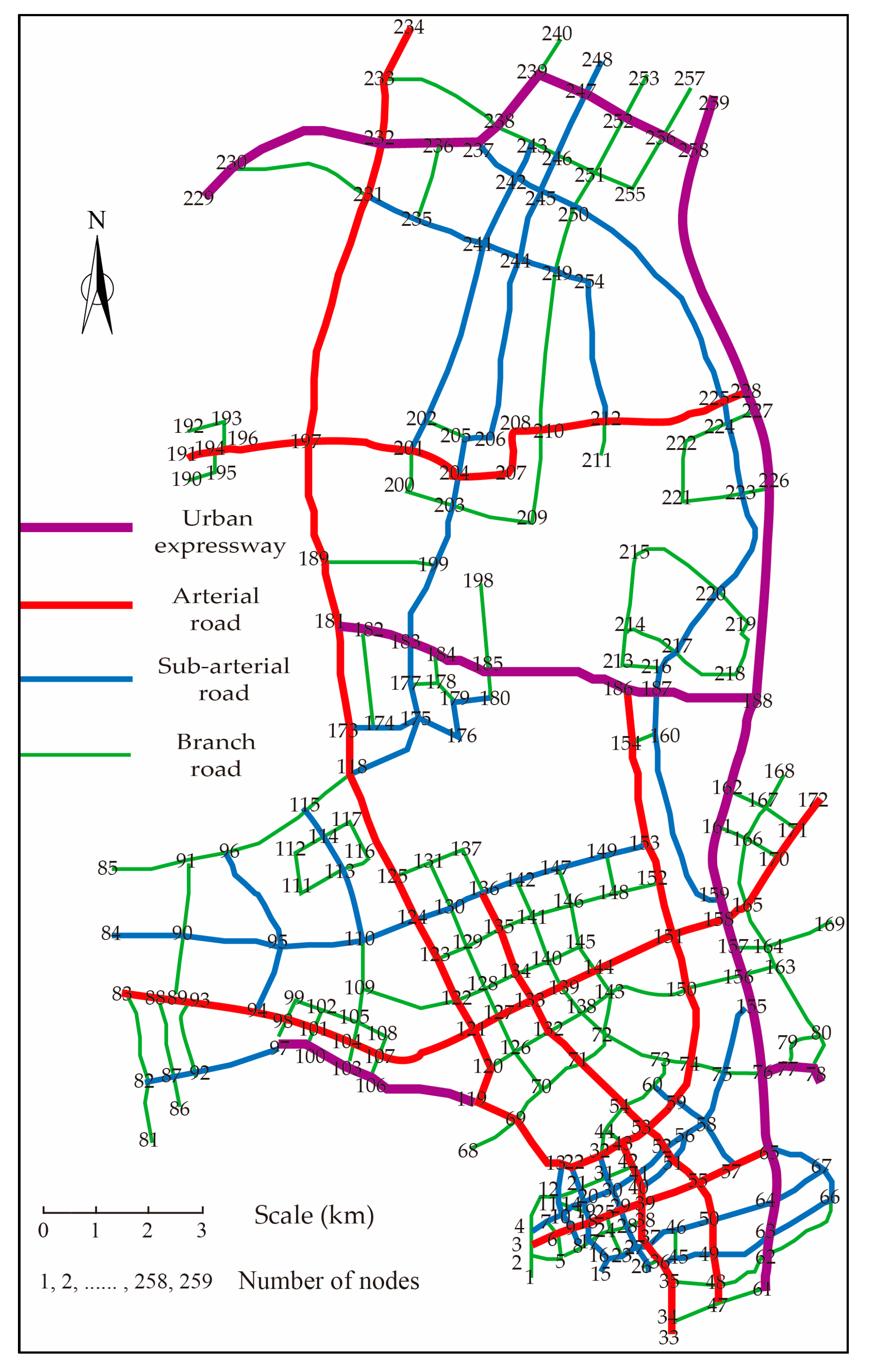
5. Case Study
5.1. Scenarios
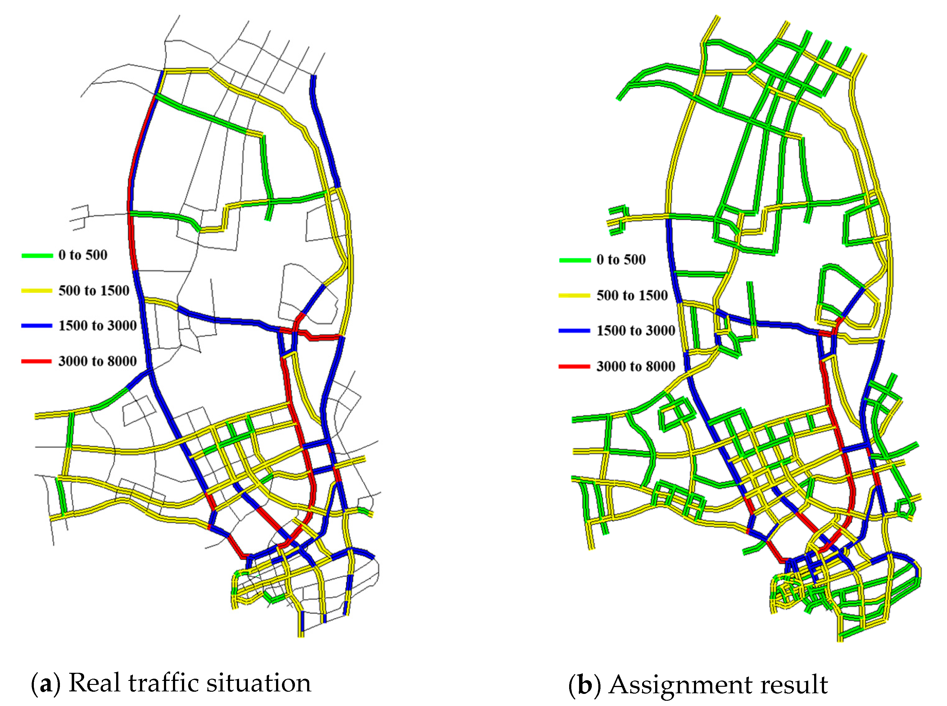
5.2. Model Validation
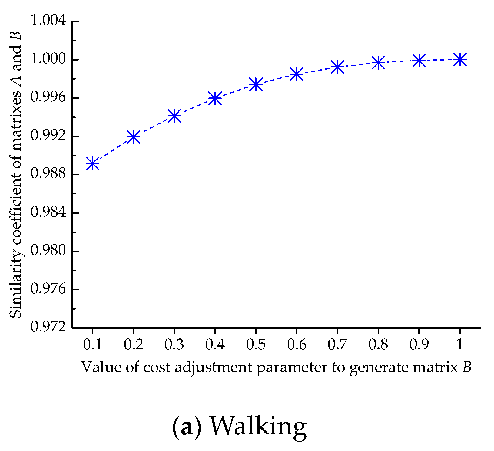
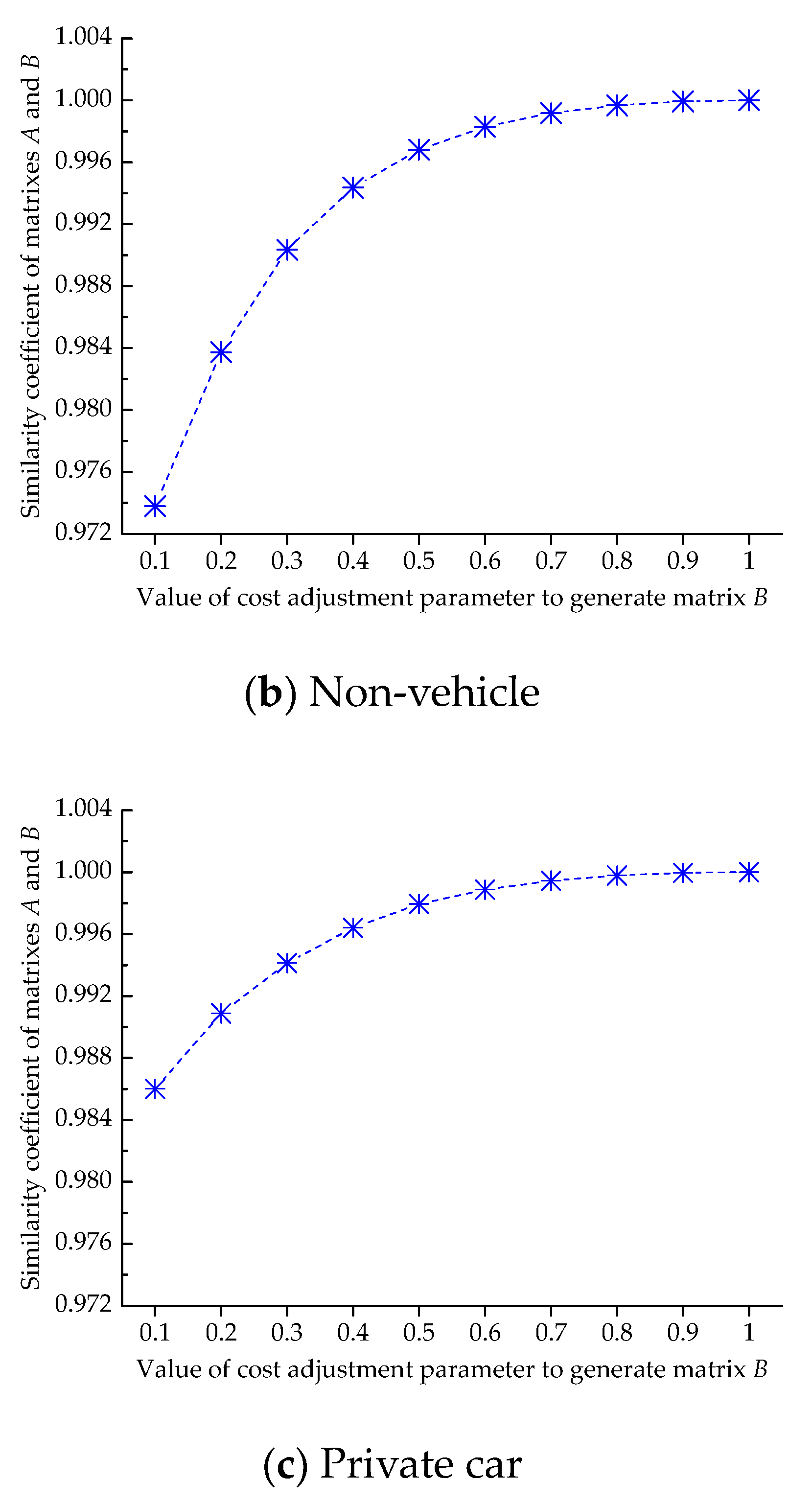
5.3. Sensitivity Analysis
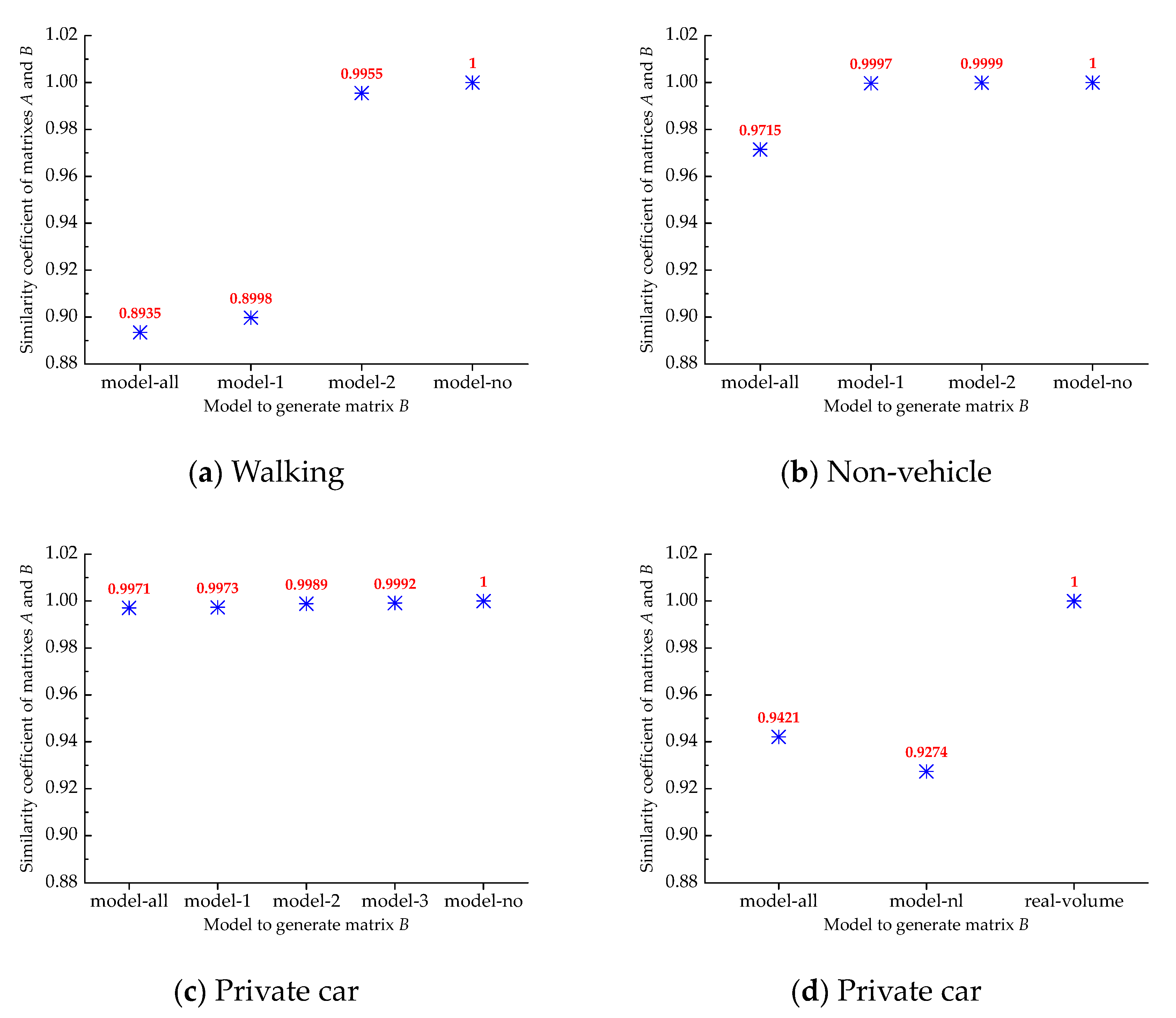
5.4. Comparison Analysis
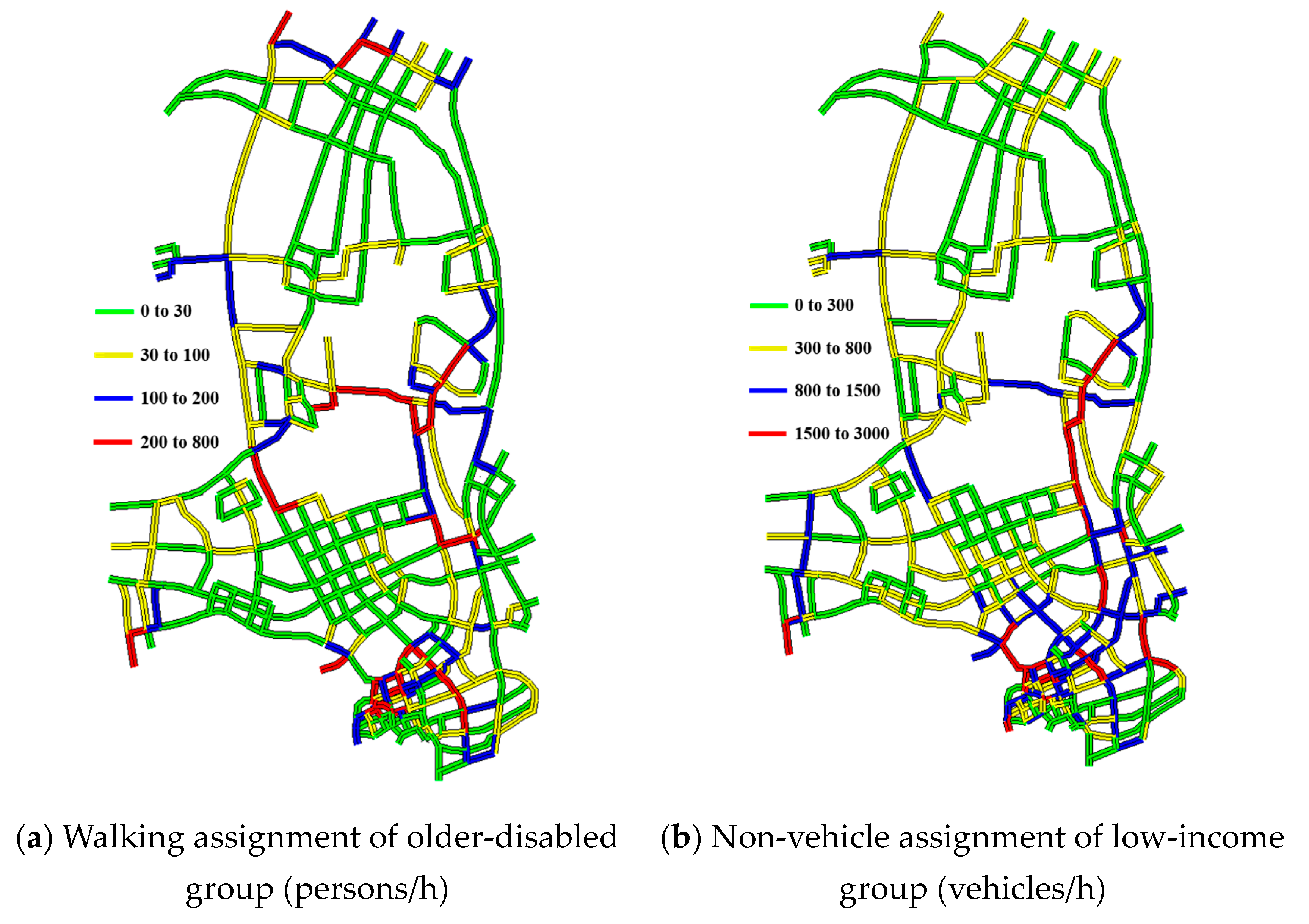
5.5. Discussion of Low-Mobility Groups
6. Conclusions
Author Contributions
Funding
Acknowledgments
Conflicts of Interest
References
- Jansuwan, S.; Christensen, K.M.; Chen, A. Assessing the transportation needs of low-mobility individuals: Case study of a small urban community in Utah. J. Urban Plan. Dev. 2013, 139, 104–114. [Google Scholar] [CrossRef]
- Ren, G.; Zhang, T.; Xu, L.; Yang, Y. Transportation demands of low-mobility individuals: Case study in Wenling, China. J. Urban Plan. Dev. 2018, 144, 05018019. [Google Scholar] [CrossRef]
- Zhang, T.; Ren, G.; Yang, Y. Transit route network design for low-mobility individuals using a hybrid metaheuristic approach. J. Adv. Transp. 2020, 2020, 7059584. [Google Scholar] [CrossRef]
- Wardrop, J.G. Some theoretical aspects of road traffic research. Proc. Inst. Civ. Eng. 1952, 1, 325–362. [Google Scholar] [CrossRef]
- LeBlanc, L.J.; Morlok, E.K.; Pierskalla, W.P. An efficient approach to solving the road network equilibrium traffic assignment problem. Transp. Res. 1975, 9, 309–318. [Google Scholar] [CrossRef]
- Daskin, M.S. Transportation networks: Equilibrium analysis with mathematical programming methods. Transp. Sci. 1985, 19, 463–466. [Google Scholar] [CrossRef]
- Patriksson, M. The Traffic Assignment Problem: Models and Methods, 2nd ed.; Dover Publications: New York, NY, USA, 2015; pp. 1–219. [Google Scholar]
- Florian, M. A traffic equilibrium model of travel by car and public transit modes. Transp. Sci. 1977, 11, 166–179. [Google Scholar] [CrossRef]
- Florian, M.; Spiess, H. On binary mode choice/assignment models. Transp. Sci. 1983, 17, 32–47. [Google Scholar] [CrossRef]
- Nagurney, A.B. Comparative tests of multimodal traffic equilibrium methods. Transp. Res. Part B Methodol. 1984, 18, 469–485. [Google Scholar] [CrossRef]
- Wong, S.C. Multi-commodity traffic assignment by continuum approximation of network flow with variable demand. Transp. Res. Part B Methodol. 1998, 32, 567–581. [Google Scholar] [CrossRef]
- Ferrari, P. A model of urban transport management. Transp. Res. Part B Methodol. 1999, 33, 43–61. [Google Scholar] [CrossRef]
- Li, S.; Deng, W.; Lv, Y. Combined modal split and assignment model for the multimodal transportation network of the economic circle in China. Transport 2009, 24, 241–248. [Google Scholar] [CrossRef]
- Florian, M.; Nguyen, S. A combined trip distribution modal split and trip assignment model. Transp. Res. 1978, 12, 241–246. [Google Scholar] [CrossRef]
- Safwat, K.N.A.; Magnanti, T.L. A combined trip generation, trip distribution, modal split, and trip assignment model. Transp. Sci. 1988, 22, 14–30. [Google Scholar] [CrossRef]
- Abrahamsson, T.; Lundqvist, L. Formulation and estimation of combined network equilibrium models with applications to Stockholm. Transp. Sci. 1999, 33, 80–100. [Google Scholar] [CrossRef]
- Fernádez, J.E.; De Cea, J.; Soto, A. A multi-model supply–demand equilibrium model for predicting intercity freight flows. Transp. Res. Part B Methodol. 2003, 37, 615–640. [Google Scholar] [CrossRef]
- Jourquin, B.; Limbourg, S. Equilibrium traffic assignment on large Virtual Networks: Implementation issues and limits for multi-modal freight transport. Eur. J. Transport. Infrastruct. Res. 2006, 6. [Google Scholar] [CrossRef]
- Uchida, K.; Sumalee, A.; Watling, D.; Connors, R. A study on network design problems for multi-modal networks by probit-based stochastic user equilibrium. Netw. Spat. Econ. 2007, 7, 213–240. [Google Scholar] [CrossRef]
- Xu, M.; Gao, Z. Multi-class multi-modal network equilibrium with regular choice behaviors: A general fixed point approach. In Transportation and Traffic Theory 2009: Golden Jubilee; Springer: Boston, MA, USA, 2009; pp. 301–325. [Google Scholar]
- Sumalee, A.; Uchida, K.; Lam, W.H.K. Stochastic multi-modal transport network under demand uncertainties and adverse weather condition. Transp. Res. Part. C Emerg. Technol. 2011, 19, 338–350. [Google Scholar] [CrossRef]
- Si, B.; Yan, X.; Sun, H.; Yang, X.; Gao, Z. Travel demand-based assignment model for multimodal and multiuser transportation system. J. Appl. Math. 2012, 2012, 592104. [Google Scholar] [CrossRef]
- Han, L.; Sun, H.; Zhu, C.; Wu, J.; Jia, B. The stability of multi-modal traffic network. Commun. Theor. Phys. 2013, 60, 48–54. [Google Scholar] [CrossRef]
- Meng, M. Traffic Assignment Model and Algorithm with Combined Modes on Urban Transportation Network. Ph.D. Thesis, Beijing Jiaotong University, Beijing, China, 2013. [Google Scholar]
- Fu, X.; Lam, W.H.K.; Chen, B.Y. A reliability-based traffic assignment model for multi-modal transport network under demand uncertainty. J. Adv. Transp. 2014, 48, 66–85. [Google Scholar] [CrossRef]
- Verbas, İ.Ö.; Mahmassani, H.S.; Hyland, M.F.; Halat, H. Integrated mode choice and dynamic traveler assignment in multimodal transit networks: Mathematical Formulation, Solution Procedure, and Large-Scale Application. Transp. Res. Rec. 2016, 2564, 7888. [Google Scholar] [CrossRef]
- Ameli, M.; Lebacque, J.P.; Leclercq, L. Multi-attribute, multi-class, trip-based, multi-modal traffic network equilibrium model: Application to large-scale network. In Proceedings of International Conference on Traffic and Granular Flow; Springer: Berlin, Germany, 2017; pp. 487–495. [Google Scholar]
- Ryu, S.; Chen, A.; Choi, K. Solving the combined modal split and traffic assignment problem with two types of transit impedance function. Eur. J. Oper. Res. 2017, 257, 870–880. [Google Scholar] [CrossRef]
- Xu, P. Intercity Multi-Modal Traffic Assignment Model and Algorithm for Urban Agglomeration Considering the Whole Travel Process; IOP Publishing: Bristol, UK, 2018; p. 062016. [Google Scholar]
- Tavassoli, A.; Mesbah, M.; Hickman, M. Calibrating a transit assignment model using smart card data in a large-scale multi-modal transit network. Transportation 2019, 1–24. [Google Scholar] [CrossRef]
- Boyce, D.E. Network Equilibrium Models of Urban Location and Travel Choices: A New Research Agenda; Palgrave Macmillan: London, UK, 1990; pp. 238–256. [Google Scholar]
- Boyce, D.E. Long-Term Advances in the State of the Art of Travel Forecasting Methods; Springer: Boston, MA, USA, 1998; pp. 73–86. [Google Scholar]
- Fernández, E.; De Cea, J.; Florian, M.; Cabrera, E. Network equilibrium models with combined modes. Transp. Sci. 1994, 28, 182–192. [Google Scholar] [CrossRef]
- Lo, H.K.; Yip, C.W.; Wam, Q.K. Modeling transfer and mon-linear fare structure in multi-modal network. Transp. Res. Part B Methodol. 2003, 37, 149–170. [Google Scholar] [CrossRef]
- Lo, H.K.; Yip, C.W.; Wam, Q.K. Modeling competitive multi-modal transit services: A nested logit approach. Transp. Res. Pt. C Emerg. Technol. 2004, 12, 251–272. [Google Scholar] [CrossRef]
- Liu, T.L.; Huang, H.J.; Yang, H.; Zhang, X. Continuum modeling of park-and-ride services in a linear monocentric city with deterministic mode choice. Transp. Res. Part B Methodol. 2009, 43, 692–707. [Google Scholar] [CrossRef]
- Abdelghany, K.; Mahmassani, H. Dynamic trip assignment-simulation model for intermodal transportation networks. Transp. Res. Rec. 2001, 1771, 52–60. [Google Scholar] [CrossRef]
- Di Gangi, M.; Polimeni, A. A model to simulate multimodality in a mesoscopic dynamic network loading framework. J. Adv. Transp. 2017, 2017, 8436821. [Google Scholar] [CrossRef]
- Florian, M.; Wu, J.H.; He, S. A Multi-Class Multi-Mode Variable Demand Network Equilibrium Model with Hierarchical Logit Structures; Springer: Boston, MA, USA, 2002; pp. 119–133. [Google Scholar]
- García, R.; Marín, A. Parking capacity and pricing in park’n ride trips: A continuous equilibrium network design problem. Ann. Oper. Res. 2002, l16, 153–178. [Google Scholar] [CrossRef]
- García, R.; Marín, A. Network equilibrium with combined modes: Models and solution algorithms. Transp. Res. Part B Methodol. 2005, 39, 223–254. [Google Scholar] [CrossRef]
- Lam, W.H.K.; Li, Z.C.; Wong, S.C.; Zhu, D. Modeling an elastic-demand bimodal transport network with park-and-ride trips. Tsinghua Sci. Technol. 2007, 12, 158–166. [Google Scholar] [CrossRef]
- Wu, Z.X.; Lam, W.H.K. Network equilibrium model for congested multi-mode networks with elastic demand. J. Adv. Transp. 2003, 37, 295–318. [Google Scholar] [CrossRef]
- Wu, Z.X.; Lam, W.H.K. A network equilibrium model for congested multimode transport network with elastic demand. In Proceedings of the 7th Conference Hong Kong Society for Transportation Studies, Hong Kong, 14 December 2002; pp. 274–283. [Google Scholar]
- Dial, R.B. A model and algorithm for multicriteria route-mode choice. Transp. Res. Part B Methodol. 1979, 13, 311–316. [Google Scholar] [CrossRef]
- Nagurney, A.; Dong, J. A multiclass, multicriteria traffic network equilibrium model with elastic demand. Transp. Res. Part B Methodol. 2002, 36, 445–469. [Google Scholar] [CrossRef]
- Lotfi, S.; Koohsari, M.J. Neighborhood walkability in a city within a developing country. J. Urban Plan. Dev. 2011, 137, 402–408. [Google Scholar] [CrossRef]
- Xie, X.F.; Smith, S.F.; Barlow, G.J. Schedule-Driven Coordination for Real-Time Traffic Network Control. In Proceedings of the Twenty-Second International Conference on International Conference on Automated Planning and Scheduling, Palaiseau, France, 25–29 June 2012. [Google Scholar]
- Xie, X.F.; Wang, Z.J. Combined traffic control and route choice optimization for traffic networks with disruptive changes. Transp. B 2019, 7, 814–833. [Google Scholar] [CrossRef]
- Zambrano-Martinez, J.L.; Calafate, C.T.; Soler, D.; Cano, J.C.; Manzoni, P. Modeling and characterization of traffic flows in urban environments. Sensors 2018, 18, 2020. [Google Scholar] [CrossRef]
- Nguyen, T.V.; Krajzewicz, D.; Fullerton, M.; Nicolay, E. DFROUTER-Estimation of Vehicle Routes from Cross-Section Measurements. In Modeling Mobility with Open Data; Springer: Berlin, Germany, 2015; pp. 3–23. [Google Scholar]
- Zambrano-Martinez, J.L.; Calafate, C.T.; Soler, D.; Cano, J.C. Towards realistic urban traffic experiments using DFROUTER: Heuristic, validation and extensions. Sensors 2017, 17, 2921. [Google Scholar] [CrossRef] [PubMed]


| Index | Urban Expressway | Arterial Road | Sub-Arterial Road | Branch Road | |
|---|---|---|---|---|---|
| Type | |||||
| Lane-width | Walking (m) | 0.9 | 2.5 | 1.5 | 0.75 |
| Non-vehicle (m) | 3.5 | 3 | 2.5 | 1.5 | |
| Vehicle (m) | 3.75 | 3.5 | 3 | 3 | |
| Number of lanes (two-way) | Walking | 2 | 2 | 2 | 2 |
| Non-vehicle | 2 | 2 | 2 | 2 | |
| Vehicle | 6 | 6 | 4 | 4 | |
| Traffic capacity (one-way) | Walking (persons/h) | 1800 | 6000 | 4000 | 1500 |
| Non-vehicle (vehicles/h) | 2400 | 2200 | 2000 | 800 | |
| Vehicle (vehicles/h) | 3900 | 3000 | 1400 | 800 | |
| Travel speed | Pedestrian (km/h) | 5.4 | 5.4 | 5.4 | 5.4 |
| Regular bike (km/h) | 10 | 10 | 10 | 8 | |
| Electric bike (km/h) | 20 | 20 | 20 | 15 | |
| Private car (km/h) | 80 | 50 | 40 | 30 | |
| Is there a traffic barricade between vehicle and non-vehicle lanes? | Yes | Yes | Yes | No | |
| Is there a traffic barricade between walking and non-vehicle lanes? | Yes | Yes | Yes | No | |
| Symbol | Description | Unit | Value | |
|---|---|---|---|---|
| Traffic volume on path p between O-D pair ij | Walking | persons/h | ||
| Non-vehicle | vehicles/h | |||
| Private car | vehicles/h | |||
| Cost adjustment parameter | 1 | |||
| Travel demand between O-D pair ij | Walking | persons/h | ||
| Non-vehicle | vehicles/h | |||
| Private car | vehicles/h | |||
| Generalized travel cost between O-D pair ij on the path p | Walking | h | ||
| Non-vehicle | min | |||
| Private car | min | |||
| Travel time on link l | Walking | h | ||
| Non-vehicle | min | |||
| Private car | min | |||
| Adjusted coefficient | 0.25 | |||
| Standard lane-width | Walking | m | 1.5 | |
| Non-vehicle | m | 1.5 | ||
| Private car | m | 3.75 | ||
| Lane-width of mode m on link l | m | |||
| Length of link l | km | |||
| Traffic capacity on link l | Walking | persons/h | ||
| Non-vehicle | vehicles/h | |||
| Private car | vehicles/h | |||
| Retardation parameter | 0.15 | |||
| Retardation parameter | 4 | |||
| Factor representing conversion between money and time | min/¥ | 1.89 | ||
| Fuel cost per unit length | ¥/km | 0.75 | ||
| Length of red light on the corresponding intersection of link l | s | |||
| Number of private cars on the corresponding intersection of link l | vehicles | |||
| Standard length of private cars | m | 7.2 | ||
| Forward crossing length of the corresponding intersection of link l | m | |||
| Coefficient related to driving direction on the corresponding intersection of link l | Turning left | 1.5 | ||
| Going forward | 1 | |||
| Turning right | 0.5 | |||
| Number of non-vehicles on the corresponding intersection of link l | vehicles | |||
| Adjustment parameter | 2.09 | |||
| Number of pedestrians crossing the corresponding intersection of link l | persons | |||
| Decision coefficient | 3 | |||
| Error parameter | 0.01 | |||
© 2020 by the authors. Licensee MDPI, Basel, Switzerland. This article is an open access article distributed under the terms and conditions of the Creative Commons Attribution (CC BY) license (http://creativecommons.org/licenses/by/4.0/).
Share and Cite
Zhang, T.; Yang, Y.; Cheng, G.; Jin, M. A Practical Traffic Assignment Model for Multimodal Transport System Considering Low-Mobility Groups. Mathematics 2020, 8, 351. https://doi.org/10.3390/math8030351
Zhang T, Yang Y, Cheng G, Jin M. A Practical Traffic Assignment Model for Multimodal Transport System Considering Low-Mobility Groups. Mathematics. 2020; 8(3):351. https://doi.org/10.3390/math8030351
Chicago/Turabian StyleZhang, Tao, Yang Yang, Gang Cheng, and Minjie Jin. 2020. "A Practical Traffic Assignment Model for Multimodal Transport System Considering Low-Mobility Groups" Mathematics 8, no. 3: 351. https://doi.org/10.3390/math8030351
APA StyleZhang, T., Yang, Y., Cheng, G., & Jin, M. (2020). A Practical Traffic Assignment Model for Multimodal Transport System Considering Low-Mobility Groups. Mathematics, 8(3), 351. https://doi.org/10.3390/math8030351