The Impact of the Discrepancy Principle on the Tikhonov-Regularized Solutions with Oversmoothing Penalties

Abstract

This paper deals with the Tikhonov regularization for nonlinear ill-posed operator equations in Hilbert scales with oversmoothing penalties. One focus is on the application of the discrepancy principle for choosing the regularization parameter and its consequences. Numerical case studies are performed in order to complement analytical results concerning the oversmoothing situation. For example, case studies are presented for exact solutions of Hölder type smoothness with a low Hölder exponent. Moreover, the regularization parameter choice using the discrepancy principle, for which rate results are proven in the oversmoothing case in in reference (Hofmann, B.; Mathé, P. Inverse Probl. 2018, 34, 015007) is compared to Hölder type a priori choices. On the other hand, well-known analytical results on the existence and convergence of regularized solutions are summarized and partially augmented. In particular, a sketch for a novel proof to derive Hölder convergence rates in the case of oversmoothing penalties is given, extending ideas from in reference (Hofmann, B.; Plato, R. ETNA. 2020, 93).

1. Introduction

This paper tries to complement the theory and practice of Tikhonov regularization with oversmoothing penalties for the stable approximate solution of nonlinear ill-posed problems in a Hilbert scale setting. Thus, we consider the operator equation

$$F\left(x\right)=y$$

(1)

with a nonlinear forward operator $F:\mathcal{D}\left(F\right)\subseteq X\to Y$, possessing the domain $\mathcal{D}\left(F\right)$ and mapping between the infinite dimensional real Hilbert spaces X and Y. In this context, ${\parallel ·\parallel }_X$ and ${\parallel ·\parallel }_Y$ denote the norms in X and Y, respectively. Throughout the paper, let $x^{†}\in \mathcal{D}\left(F\right)$ be a solution to Equation (1) for a given right-hand side y. We restrict our considerations to problems that are locally ill-posed at $x^{†}$. This means that the replacement of the exact right-hand side y by noisy data $y^{\delta }\in Y$, obeying the deterministic noise model

$$\parallel y-y^{\delta }{\parallel }_Y\le \delta$$

(2)

with noise level $\delta >0$, may lead to significant errors in the solution of Equation (1) measured by the X-norm, even if $\delta$ tends to zero (cf. ([1], Def. 2) for details).

For finding approximate solutions, we apply a Hilbert scale setting, where the densely defined, unbounded and self-adjoint linear operator $B:\mathcal{D}\left(B\right)\subset X\to X$ with domain $\mathcal{D}\left(B\right)$ generates the Hilbert scale. This operator is assumed to be strictly positive such that we have for some $\underline{m}>0$

$${\parallel Bx\parallel }_X\ge \underline{m}{\parallel x\parallel }_X,\mathrm{for}\mathrm{all}x\in \mathcal{D}\left(B\right).$$

(3)

In this sense, we exploit the Hilbert scale ${\left\{X_{\tau }\right\}}_{\tau \in \mathbb{R}}$ generated by B with $X_0=X$, $X_{\tau }=\mathcal{D}\left(B^{\tau }\right)$, and with corresponding norms ${\parallel x\parallel }_{\tau }:={\parallel B^{\tau }x\parallel }_X$.

As approximate solutions to $x^{†}$, we use Tikhonov-regularized solutions $x_{\alpha }^{\delta }\in \mathcal{D}\left(F\right)$ that are minimizers of the extremal problem

$$T_{\alpha }^{\delta }\left(x\right):=\parallel F\left(x\right)-y^{\delta }{\parallel }_Y^2+\alpha {\parallel Bx\parallel }_X^2\to min,\mathrm{subject}\mathrm{to}x\in \mathcal{D}:=\mathcal{D}\left(F\right)\cap \mathcal{D}\left(B\right),$$

(4)

where $\alpha >0$ is the regularization parameter and $\parallel F\left(x\right)-y^{\delta }{\parallel }_Y^2$ characterizes the misfit or fidelity term. The penalty functional ${\parallel Bx\parallel }_X^2={\parallel x\parallel }_1^2$ in the Tikhonov functional $T_{\alpha }^{\delta }$ is adjusted to the level one of Hilbert scale such that all regularized solutions have the property $x_{\alpha }^{\delta }\in \mathcal{D}\left(B\right)$. A more general form of the penalty functional in the Tikhonov functional would be $\parallel B(x-\overline{x}){\parallel }_X^2$, where $\overline{x}\in \mathcal{D}$ denotes a given smooth reference element. $\overline{x}$ then plays the role of the origin (the point of central interest), which can be very different for nonlinear problems. Without a loss of generality, we set in the sequel $\overline{x}:=0,$ which makes the formulas simpler.

In our study, the discrepancy principle named after Morozov (cf. [2]) as the most prominent a posteriori choice of the regularization parameter $\alpha >0$ plays a substantial role. On the one hand, the simplified version

$${\alpha }_{discr}:=\alpha (\delta ,y^{\delta }):{\parallel F\left(x_{{\alpha }_{discr}}^{\delta }\right)-y^{\delta }\parallel }_Y=C\delta$$

(5)

of the discrepancy principle in equation form with a prescribed constant $C>1$ is important for theory (cf. [3]). However, it is well known that there are nonlinear problems, where that version is problematic due to duality gaps that prevent the solvability of Equation (5). For overcoming the remaining weaknesses of the parameter choice expressed in Equation (5), sequential versions of the discrepancy principle can be applied that approximate ${\alpha }_{discr}$, and we refer to [4,5,6] for more details. Such an approach is used for performing the numerical case studies in Section 6.

Our focus is on oversmoothing penalties in the Tikhonov functional $T_{\alpha }^{\delta }$, where $x^{†}\notin \mathcal{D}\left(B\right)=X_1$ such that $T_{\alpha }^{\delta }\left(x^{†}\right)=\infty$. In this case, the regularizing property $T_{\alpha }^{\delta }\left(x_{\alpha }^{\delta }\right)\le T_{\alpha }^{\delta }\left(x^{†}\right)$ does not yield any information. This property, however, is the basic tool for obtaining error estimates and convergence assertions for the Tikhonov-regularized solutions in the standard case, where $T_{\alpha }^{\delta }\left(x^{†}\right)<\infty$. We refer as an example to Chapter 10 of the monograph [7], which also deals with nonlinear operator equations, but adjusts the penalty functional to level zero. To derive error estimates in the oversmoothing case, the regularizing property must be replaced by inequalities of the form $T_{\alpha }^{\delta }\left(x_{\alpha }^{\delta }\right)\le T_{\alpha }^{\delta }\left(x_{aux}\right)$, where $x_{aux}\in \mathcal{D}$ is an appropriately chosen auxiliary element.

The seminal paper on Tikhonov regularization in Hilbert scales that includes the oversmoothing case was written by F. Natterer in 1984 (cf. [8]) and was restricted to linear operator equations. Error estimates in the X-norm and convergence rates were proven under two-sided inequalities that characterize the degree of ill-posedness $a>0$ of the problem. We follow this approach and adapt it to the case of nonlinear problems throughout the subsequent sections and assume the inequality chain

$$c_a\parallel x-x^{†}{\parallel }_{-a}\le \parallel F\left(x\right)-F\left(x^{†}\right){\parallel }_Y\le C_a{\parallel x-x^{†}\parallel }_{-a}\mathrm{for}\mathrm{all}x\in \mathcal{D}$$

(6)

and constants $0<c_a\le C_a<\infty$. The left-hand inequality in Equation (6) represents a conditional stability estimate and is substantial for obtaining stable regularized solutions, whereas the right-hand inequality in Equation (6) contributes to the determination of the nonlinearity structure of the forward operator F. Convergence and rate results for the Tikhonov regularization expressed in Equation (4) with oversmoothing penalties under the inequality chain expressed in Equation (6) were recently presented in [3,6,9] and complemented by case studies in [10]. The present paper continues this series of articles by addressing open questions with respect to the discrepancy principle for choosing the regularization parameter $\alpha$ and its comparison to a priori parameter choices. In this context, one of the examples from [10] is reused for performing new numerical experiments in order to obtain additional assertions that cannot be taken from analytical investigations.

The paper is organized as follows: We summarize in Section 2 basic properties of regularized solutions under assumptions that are typical for oversmoothing penalties and in Section 3 assertions concerning the convergence. In Section 4 we show that the error estimates derived in [6] for obtaining low order convergence rates are also applicable to obtain the order optimal Hölder convergence rates under the associated Hölder-type source conditions. Section 5 recalls a nonlinear inverse problem from an exponential growth model and an appropriate Hilbert scale, which can both be used for performing numerical experiments in the subsequent section. In that section (Section 6), the obtained numerical results are presented and interpreted based on a series of tables and figures.

2. Assumptions and Properties of Regularized Solutions

In this section, we formulate the standing assumptions concerning the forward operator F, the Tikhonov functional $T_{\alpha }^{\delta }$, and the solution $x^{†}$ of Equation (1) in order to ensure the existence and stability of regularized solutions $x_{\alpha }^{\delta }$ for all regularization parameters $\alpha >0$ and noisy data $y^{\delta }$.

Assumption 1.

(a)

The operator$F:\mathcal{D}\left(F\right)\subseteq X\to Y$mapping between the real Hilbert spaces X and Y is weakly sequentially continuous, and its domain$\mathcal{D}\left(F\right)$with$0\in \mathcal{D}\left(F\right)$is a convex and closed subset of X.

(b)

The generator$B:\mathcal{D}\left(B\right)\subset X\to X$of the Hilbert scale is a densely defined, unbounded, and self-adjoint linear operator that satisfies the inequality expressed in Equation (3).

(c)

The solution$x^{†}\in \mathcal{D}\left(F\right)$of Equation (1) is supposed to be an interior point of the domain$\mathcal{D}\left(F\right)$.

(d)

To characterize the case of oversmoothing penalties, we assume that

$$x^{†}\notin \mathcal{D}\left(B\right)=X_1.$$

(7)

(e)

There is a number $a>0$, and there are constants $0<c_a\le C_a<\infty$such that the two-sided estimates expressed in Equation (6) hold.

As a specific impact of Item (d) of Assumption 1 on approximate solutions to $x^{†}$, we have the following proposition that is of interest for the behavior of regularized solutions in the case of oversmoothing penalties.

Proposition 1.

Let a sequence $\left\{x_n\right\}\subset \mathcal{D}\left(B\right)\subset X$ converge weakly in X to $x^{†}\notin \mathcal{D}\left(B\right)$ as $n\to \infty$. We then have $\underset{n\to \infty }{lim}{\parallel B{x}_n\parallel }_X=\infty$.

Proof. 

In order to construct a contradiction, let us assume that the sequence $\left\{x_n\right\}\subset \mathcal{D}\left(B\right)$ (or some of its subsequences) is bounded in $X_1$, i.e., $\parallel B{x}_n{\parallel }_X\le K$ for all $n\in \mathbb{N}$. Thus, a subsequence of $\left\{B{x}_n\right\}$ converges weakly in X to some element $z\in X$, because bounded sets are weakly pre-compact in the Hilbert space X. Since the operator B is densely defined and self-adjoint, it is closed, i.e., the graph $\left\{\right(x,Bx):x\in \mathcal{D}(B\left)\right\}$ is closed and, due to the convexity of this set, a weakly closed subset of $X\times Y$. Hence, the operator B is weakly closed, which implies that $x^{†}\in \mathcal{D}\left(B\right)$ and $B{x}^{†}=z$. This, however, contradicts the assumed property $x^{†}\notin \mathcal{D}\left(B\right)$ and proves the proposition. ☐

Remark 1.

As a consequence of Proposition 1, we have for any sequence of regularized solutions $\{x_n=x_{{\alpha }_n}^{{\delta }_n}\}$, which is norm-convergent (and thus also weak-convergent) to $x^{†}\notin \mathcal{D}\left(B\right)$ for ${\delta }_n\to 0$ as $n\to \infty$, such that it blows up to infinity with respect to the $X_1$-norm. In other words, we have the limit condition $\underset{n\to \infty }{lim}\parallel B{x}_{{\alpha }_n}^{{\delta }_n}{\parallel }_X={\parallel B{x}^{†}\parallel }_X=\infty$.

Based on Lemma 1, we can formulate in Proposition 2 the existence of minimizers to the extremal problem expressed in Equation (4).

Lemma 1.

The non-negative penalty functional ${\parallel B·\parallel }_X^2:\mathcal{D}\left(B\right)\subset X\to \mathbb{R}$ as part of the Tikhonov functional $T_{\alpha }^{\delta }$ is a proper convex and a lower, semi-continuous, and stabilizing functional.

Proof. 

The obviously convex penalty functional is proper, since it attains finite values for all $x\in \mathcal{D}\left(B\right)=X_1\ne \varnothing$. It is also a stabilizing functional because, as a consequence of Equation (3), the sub-level sets $\{x\in \mathcal{D}\left(B\right):\parallel Bx{\parallel }_X^2\le c\}$ are weakly sequentially pre-compact subsets in X for all constants $c\ge 0$. Namely, all such non-empty sub-level sets are bounded in X and hence weakly pre-compact. For showing that the functional ${\parallel B·\parallel }_X^2={\parallel ·\parallel }_1^2$ is lower semi-continuous, by taking into account Proposition 1 and its proof, it is enough to show that a sequence $\left\{x_n\right\}\subset \mathcal{D}\left(B\right)$ with $\parallel x_n{\parallel }_1\le K<\infty$ for all $n\in \mathbb{N}$ that converges weakly in X to $\widehat{x}\in X$ implies that $\widehat{x}\in \mathcal{D}\left(B\right)$ and that this sequence also converges weakly in $X_1$ to $\widehat{x}$. The lower semi-continuity of the norm functional ${\parallel ·\parallel }_1$ then yields $\parallel B\widehat{x}{\parallel }_X^2\le \underset{n\to \infty }{lim\; inf}{\parallel B{x}_n\parallel }_X^2$. Now note that a subsequence $\left\{x_n\right\}$ bounded in $X_1$ has a subsequence that converges weakly in $X_1$ to some element $z\in X_1$. Since the operator B is weakly closed, we then have $B\widehat{x}=z$. Since z is uniform for all subsequences, this completes the proof. ☐

Proposition 2.

For all $\alpha >0$ and $y^{\delta }\in Y$, there is a regularized solution $x_{\alpha }^{\delta }\in \mathcal{D}$, solving the extremal problem expressed in Equation (4).

Proof. 

Proposition 4.1 from [11], which coincides with our proposition, is immediately applicable, since the Assumptions 3.11 and 3.22 from [11] are satisfied due to Assumption 1 and Lemma 1 above. ☐

In addition to the existence assertion of Proposition 2, we also have, under the assumptions stated above, the stability of regularized solutions, which means that small changes in the data $y^{\delta }$ yield only small changes in $x_{\alpha }^{\delta }$. For a detailed description of this fact, see Proposition 4.2 from [11] that applies here under Assumption 1.

Remark 2.

From Assumption 1, we have that there are no solutions $x^{\ast }\in \mathcal{D}=\mathcal{D}\left(F\right)\cap \mathcal{D}\left(B\right)$, satisfying with $F\left(x^{\ast }\right)=y$ the operator expressed in Equation (1), because this would contradict, with $F\left(x^{†}\right)=F\left(x^{\ast }\right)$ and $\parallel x^{†}-x^{\ast }{\parallel }_X>0$, the left-hand inequality of Equation (6). Besides $x^{†}$, however, other solutions with $x^{\ast }\notin \mathcal{D}\left(B\right)$ may exist. The regularized solutions $x_{\alpha }^{\delta }$, for fixed $\alpha >0$ and $y^{\delta }\in Y$, need not be uniquely determined, since, though possessing a convex part ${\parallel Bx\parallel }^2$, the Tikhonov functional $T_{\alpha }^{\delta }\left(x\right)$ is not necessarily convex.

3. Convergence of Regularized Solutions in the Case of Oversmoothing Penalties

In this section, we discuss assertions about the X-norm convergence of regularized solutions with the Tikhonov functional $T_{\alpha }^{\delta }$ introduced in Equation (4). First we recall the following lemma (from [6], Proposition 3.4).

Lemma 2.

Under Assumption 1, we have, for regularized solutions $x_{\alpha }^{\delta }\in \mathcal{D}$ solving the extremal problem expressed in Equation (4), a function $\phi :[0,\infty )\to [0,\infty )$ satisfying the limit condition $\underset{\alpha \to 0}{lim}\phi \left(\alpha \right)=0$ and a constant $\overline{K}>0$ such that the error estimate

$$\parallel x_{\alpha }^{\delta }-x^{†}{\parallel }_X\le \phi \left(\alpha \right)+\overline{K}\frac{\delta }{{\alpha }^{a/(2a+2)}}$$

(8)

is valid for all $\delta >0$ and for sufficiently small $\alpha >0$.

From Lemma 2, we directly obtain the following proposition (cf. [6], Theorem 4.1):

Theorem 1.

For any a priori parameter choice ${\alpha }_{\ast }=\alpha \left(\delta \right)$ and any a posteriori parameter choice ${\alpha }_{\ast }=\alpha (\delta ,y^{\delta })$, the regularized solutions $x_{{\alpha }_{\ast }}^{\delta }$ converge under Assumption 1 to the solution $x^{†}$ of the operator expressed in Equation (1) for $\delta \to 0$, i.e.,

$$\underset{\delta \to 0}{lim}{\parallel x_{{\alpha }_{\ast }}^{\delta }-x^{†}\parallel }_X=0,$$

(9)

whenever

$${\alpha }_{\ast }\to 0and\frac{{\delta }^2}{{\alpha }_{\ast }^{a/(a+1)}}\to 0as\delta \to 0.$$

(10)

Remark 3.

By inspection of the corresponding proofs in [6], it becomes clear that the validity of Lemma 2 and consequently of Theorem 1 is not restricted to the case of oversmoothing penalties, but it holds if Items (a), (b), (c), and (e) of Assumption 1 are fulfilled. This means that the solution $x^{†}\in \mathcal{D}\left(F\right)$ can possess arbitrary smoothness.

Example 1.

In this example, we consider with respect to Theorem 1 the a priori parameter choice

$${\alpha }_{\ast }=\alpha \left(\delta \right)\sim {\delta }^{\kappa }$$

(11)

for varying exponents $\kappa >0$. As the following proposition, as a consequence of Theorem 1, indicates, there is a wide range of exponents $\kappa$ yielding convergence.

Proposition 3.

For the a priori choice expressed in Equation (11) of the regularization parameter $\alpha >0$, the condition expressed in Equation (10) in Theorem 1 holds if and only if $0<\kappa <2+\frac{2}{a}$.

However, the proof of the underlying Theorem 4.1 in [6] shows that the general verification of the basic estimate expressed in Equation (8), developed with a focus on the case of oversmoothing penalties, requires both the left-hand inequality as well as the right-hand inequality in the nonlinearity condition expressed in Equation (6) and, moreover, that $x^{†}$ is an interior point of $\mathcal{D}\left(F\right)$. More discussions in that direction can be made if we distinguish the following three $\kappa$-intervals:

(i):

$0<\kappa <2\mathrm{with}$

$${\alpha }_{\ast }\to 0\mathrm{and}\frac{{\delta }^2}{{\alpha }_{\ast }}\to 0\mathrm{as}\delta \to 0.$$

(12)

(ii):

$\kappa =2$ with two constants $\underline{c}$ and $\overline{c}$ such that

$${\alpha }_{\ast }\to 0\mathrm{and}0<\underline{c}\le \frac{{\delta }^2}{{\alpha }_{\ast }}\le \overline{c}<\infty \mathrm{for} \mathrm{all}\delta >0.$$

(13)

and

(iii):

$2<\kappa <2+\frac{2}{a}\mathrm{with}$

$${\alpha }_{\ast }\to 0\mathrm{and}\frac{{\delta }^2}{{\alpha }_{\ast }}\to \infty \mathrm{as}\delta \to 0.$$

(14)

If we have $x^{†}\in X_1$ in contrast to Item (d) of Assumption 1, then, for the convergence of regularized solutions to $x^{†}$ in Case (i), the nonlinearity condition expressed in Equation (6) is not needed at all provided that Items (a) and (b) of Assumption 1 are fulfilled. Also Item (c) is not necessary there. However to derive Equation (9), $x^{†}$ must be the uniquely determined penalty-minimizing solution to Equation (1) (cf. [11], Sect. 4.1.2 or alternatively [12,13]). Note that, for $x^{†}\in X_1$ and parameter choices according to (i), conditions of the type expressed in Equation (6) are only relevant for proving convergence rates.

If regularization parameters are chosen such that Equation (12) is violated as in Cases (ii) and (iii), then even for $x^{†}\in X_1$ inequalities from the condition expressed in Equation (6) are important. Precisely, Case (iii) seems to require both inequalities of Equation (6) for deriving convergence of regularized solutions to $x^{†}$. The parameter choice according to Case (ii) with ${\alpha }_{\ast }=\alpha \left(\delta \right)\sim {\delta }^2$ represents for $x^{†}\in X_1$ the typical conditional stability estimate situation introduced in the seminal paper [14]. There, only the left-hand inequality of condition expressed in Equation (6) is needed for convergence, which then is a consequence of convergence rate results (cf. [15,16,17] and references therein). However, to derive Equation (9), $x^{†}$ must be the uniquely determined solution to Equation (1). In the oversmoothing case $x^{†}\notin X_1$, both inequalities in Equation (6) seem to be indispensable for obtaining convergence; moreover, for all suggested choices of the regularization parameter $\alpha$, the convergence proofs published by now, all using auxiliary elements, are essentially based on the fact that $x^{†}$ is an interior point of the domain $\mathcal{D}\left(F\right)$. Determining the conditions under which convergence takes place if $\kappa \ge 2+2/a$ is chosen in Equation (11) is an open problem.

Now we turn to convergence assertions, provided that the regularization parameter $\alpha >0$ is selected according to the discrepancy principle expressed in Equation (5) with prescribed constant $C>1$. The main ideas of the proof are outlined along the lines of [6], Theorem 4.9, where a sequential discrepancy has been considered.

Theorem 2.

Under Assumption 1, let there be, for a sequence $\left\{{\delta }_n\right\}$ of positive noise levels with ${lim}_{n\to \infty }{\delta }_n=0$ and all admissible noisy data $y^{{\delta }_n}\in Y$ obeying $\parallel y^{{\delta }_n}{-y\parallel }_Y\le {\delta }_n$, regularization parameters ${\alpha }_n:={\alpha }_{discr}({\delta }_n,y^{{\delta }_n})>0$, satisfying the discrepancy principle

$$\parallel F\left(x_{{\alpha }_n}^{{\delta }_n}\right)-y^{{\delta }_n}{\parallel }_Y=C{\delta }_n$$

(15)

for a prescribed constant $C>1$. We then have

$$\underset{n\to \infty }{lim}{\alpha }_n=0$$

(16)

and convergence as

$$\underset{n\to \infty }{lim}{\parallel x_{{\alpha }_n}^{{\delta }_n}-x^{†}\parallel }_X=0.$$

(17)

Proof. 

First, we show that Equation (16) always takes place for oversmoothing penalties with $x^{†}\notin \mathcal{D}\left(B\right)=X_1$. To find a contradiction, we assume that ${lim\; inf}_{n\to \infty }{\alpha }_n>0$. Since $0\in \mathcal{D}$ as a consequence of Item (a) of Assumption 1, we have $T_{{\alpha }_n}^{{\delta }_n}\left(x_{{\alpha }_n}^{{\delta }_n}\right)\le T_{{\alpha }_n}^{{\delta }_n}\left(0\right)$ and thus ${\alpha }_n\parallel x_{{\alpha }_n}^{{\delta }_n}{\parallel }_1^2\le \parallel F\left(0\right)-y^{{\delta }_n}{\parallel }_Y^2\le {2(\parallel F\left(0\right)-y\parallel }_Y^2+{\delta }_n^2)$, which means that $\parallel x_{{\alpha }_n}^{{\delta }_n}{\parallel }_1={\parallel B{x}_{{\alpha }_n}^{{\delta }_n}\parallel }_X$ and, by Equation (3), $\parallel x_{{\alpha }_n}^{{\delta }_n}{\parallel }_X$ are uniformly bounded from above for all $n\in \mathbb{N}$. We then have for a subsequence the weak convergences in X as $x_{{\alpha }_{n_k}}^{{\delta }_{n_k}}\rightharpoonup \tilde{x}\in X$ and $B{x}_{{\alpha }_n}^{{\delta }_n}\rightharpoonup \tilde{\tilde{x}}\in X$ as $k\to \infty$. Since the operator B is weakly sequentially closed, we therefore obtain $\tilde{x}\in \mathcal{D}\left(B\right)$ and for F weakly sequentially continuous (cf. Item (a) of Assumption 1) also $F\left(x_{{\alpha }_{n_k}}^{{\delta }_{n_k}}\right)\rightharpoonup F\left(\tilde{x}\right)$. Now, by Equation (15), we easily derive that $\parallel F\left(x_{{\alpha }_{n_k}}^{{\delta }_{n_k}}\right)-F\left(x^{†}\right){\parallel }_Y\to 0$ as $k\to \infty$ and consequently $F\left(\tilde{x}\right)=F\left(x^{†}\right)$. Thus, the left-hand inequality of Equation (6) (cf. Item (e) of Assumption 1) yields $\tilde{x}=x^{†}$, which contradicts the assumption $x^{†}\notin \mathcal{D}\left(B\right)$ and proves the property expressed in Equation (16) of the regularization parameter choice.

Secondly, we prove the convergence property expressed in Equation (17). From [6], Lemma 3.2, we have that

$$\parallel F\left(x_{{\alpha }_n}^{{\delta }_n}\right)-y^{{\delta }_n}{\parallel }_Y\le \psi \left({\alpha }_n\right){\alpha }_n^{a/(2a+2)}+{\delta }_n$$

for some function $\psi :[0,\infty )\to [0,\infty )$ satisfying the limit condition $\underset{\alpha \to 0}{lim}\psi \left(\alpha \right)=0$, for sufficiently small ${\alpha }_n>0$ and arbitrary ${\delta }_n>0$. In combination with $\parallel F\left(x_{{\alpha }_n}^{{\delta }_n}\right)-y^{{\delta }_n}{\parallel }_Y=C{\delta }_n$, this yields under the condition expressed in Equation (16), implying ${lim}_{n\to \infty }\psi \left({\alpha }_n\right)=0$ the estimate

$$\frac{{\delta }_n}{{\alpha }_n^{a/(2a+2)}}\le \frac{\psi \left({\alpha }_n\right)}{C-1}\to 0\mathrm{as}n\to \infty .$$

Now Theorem 1 applies. This completes the proof. ☐

Remark 4.

In the case $x^{†}\in X_1$ of non-oversmoothing penalties, the limit condition expressed in Equation (16) represents a canonical situation for regularized solutions, whereas the non-existence of ${\alpha }_{discr}$ from Equation (5) and the violation of Equation (16) only occur in exceptional cases. For the sequential variant of the discrepancy principle, the exceptional case ${lim\; inf}_{n\to \infty }{a}_n>0$ is discussed in [4] in the context of the exact penalization veto introduced there.

4. An Alternative Approach to Prove Hölder Convergence Rates in the Case of Oversmoothing Penalties for an A Priori Parameter Choice of the Regularization Parameter

In this section, we consider order optimal convergence rate results in the case of oversmoothing penalties for an a priori parameter choice of the regularization parameter $\alpha >0$. Such results have been proven in the paper [9] under the condition $x^{†}\in X_p=\mathcal{D}\left(B^p\right)=\mathcal{R}\left(B^{-p}\right)$ for $0<p<1$, which is a Hölder-type source condition. In that paper, the proof is formulated for the penalty $\parallel B(x-\overline{x}){\parallel }_X^2$ with reference element $\overline{x}\in \mathcal{D}$. This proof has been repeated in the appendix of the paper [10] in the simplified version with $\overline{x}=0$ and penalty term ${\parallel Bx\parallel }_X^2$, which is also utilized in the present work.

In the following, we present the sketch of an alternative proof for the order optimal Hölder convergence rates under the Hölder-type source condition $x^{†}\in X_p$ for $0<p<1$. This alternative approach is based on error estimates that have been verified in [6] for showing convergence of the regularized solutions $x_{\alpha }^{\delta }$ to $x^{†}$ and for proving low order (e.g., logarithmic) convergence rates under corresponding low order source conditions. By one novel idea outlined below, the results from [6] can be extended to prove Hölder convergence rates, too.

For the subsequent investigations, we complement Assumption 1 with an assumption that specifies the smoothness of the solution $x^{†}$:

Assumption A2.

There are $0<p<1$ and $w\in X$ such that

$$x^{†}=B^{-p}w\in X_p.$$

(18)

Theorem 3.

Under Assumptions 1 and 2, we have for the a priori parameter choice

$${\alpha }_{\ast }=\alpha \left(\delta \right)\sim {\delta }^{\frac{2(a+1)}{a+p}}$$

(19)

the convergence rate

$$\parallel x_{{\alpha }_{\ast }}^{\delta }-x^{†}{\parallel }_X=\mathcal{O}\left({\delta }^{\frac{p}{a+p}}\right)as\delta \to 0.$$

(20)

Proof. 

We give only a sketch of a proof for this theorem, presupposing the results of the recent paper [6]. Precisely, we outline only the points, where we amend and complement the results of [6] in order to extend [6], Theorem 5.3, to the case of appropriate power-type functions $\phi$.

Auxiliary elements $z_{\alpha }\in \mathcal{D}\left(B\right)$, which are for all $\alpha >0$ the uniquely determined minimizers of the artificial Tikhonov functional $T_{\alpha ,a}:=\parallel x-x^{†}{\parallel }_{-a}^2+\alpha {\parallel Bx\parallel }_X^2$, represent, in combination with the moment inequality, the essential tool for the proof. By introducing the self-adjoint and positive semi-definite bounded linear operator $G:=B^{-(2a+2)}:X\to X$, we can verify these elements in an explicit manner as

$$z_{\alpha }=G{(G+\alpha I)}^{-1}{x}^{†}=x^{†}-\alpha {(G+\alpha I)}^{-1}{x}^{†},$$

which implies that, for all $\alpha >0$,

$$z_{\alpha }-x^{†}=-\alpha {(G+\alpha I)}^{-1}{x}^{†},$$

$$B^{-a}(z_{\alpha }-x^{†})=-G^{a/(2a+2)}\left[\alpha {(G+\alpha I)}^{-1}{x}^{†}\right],$$

and

$$B(z_{\alpha }-x^{†})=G^{(2a+1)/(2a+2)}\left[\alpha {(G+\alpha I)}^{-1}{x}^{†}\right].$$

According to [6], Lemma 3.1, we then have the functions $f_1\left(\alpha \right)=o\left(1\right),f_2\left(\alpha \right)=o\left(1\right)$ and $f_3\left(\alpha \right)=o\left(1\right)$ as $\alpha \to 0$ introduced there, which can be found in our notation from the representations $\parallel z_{\alpha }-x^{†}{\parallel }_X=f_1\left(\alpha \right)$, $\parallel B^{-a}(z_{\alpha }-x^{†}){\parallel }_X=f_2\left(\alpha \right){\alpha }^{a/(2a+2)}$, and $\parallel B(z_{\alpha }-x^{†}){\parallel }_X=f_3\left(\alpha \right){\alpha }^{-1/(2a+2)}$. Under the source condition expressed in Equation (18), which attains the form $x^{†}=G^{p/(2a+2)}w$ with some source element $w\in X$, we derive in detail the formulas

$$f_1\left(\alpha \right)={\parallel G^{p/(2a+2)}\left[\alpha {(G+\alpha I)}^{-1}w\right]\parallel }_X=\mathcal{O}\left({\alpha }^{\frac{p}{2a+2}}\right)\mathrm{as}\alpha \to 0,$$

(21)

$$f_2\left(\alpha \right)={\alpha }^{-a/(2a+2)}{\parallel G^{(a+p)/(2a+2)}\left[\alpha {(G+\alpha I)}^{-1}w\right]\parallel }_X=\mathcal{O}\left({\alpha }^{\frac{p}{2a+2}}\right)\mathrm{as}\alpha \to 0,$$

(22)

and

$$f_3\left(\alpha \right)={\alpha }^{-(2a+1)/(2a+2)}{\parallel G^{(2a+1+p)/(2a+2)}\left[\alpha {(G+\alpha I)}^{-1}w\right]\parallel }_X=\mathcal{O}\left({\alpha }^{\frac{p}{2a+2}}\right)\mathrm{as}\alpha \to 0.$$

(23)

The asymptotics $\mathcal{O}\left({\alpha }^{p/(2a+2)}\right)$ in Equations (21)–(23) is a consequence of the properties ${\parallel G(G+\alpha I)}^{-1}\parallel \le 1$, ${\parallel (G+\alpha I)}^{-1}\parallel \le 1/\alpha$, which yield by exploiting the moment inequality (cf. [7], Formula (2.49))

$$\parallel G^{\theta }{(G+\alpha I)}^{-1}{\parallel \le \parallel G(G+\alpha I)}^{-1}{\parallel }^{\theta }{\parallel {(G+\alpha I)}^{-1}\parallel }^{1-\theta }\le {\alpha }^{\theta -1},\mathrm{for}\alpha >0\mathrm{and}0\le \theta \le 1$$

(24)

for the self-adjoint and positive semi-definite operator G. Here, $\parallel ·\parallel$ denotes the operator norm in the space of bounded linear operators mapping in X. In Equation (21), the inequality expressed in Equation (24) is applied with $\theta =p/(2a+2)$, it is applied with $\theta =(a+p)/(2a+2)$ in Equation (22), and it is applied with $\theta =(2a+p+1)/(2a+2)$ in Equation (23), taking into account that all three $\theta$-values are smaller than one. These are the new ideas of the present proof.

Because the function $f_9\left(\alpha \right)$ in [6], Formula (3.12), is found by linear combination and maximum-building of the functions $f_1\left(\alpha \right),f_2\left(\alpha \right)$, and $f_3\left(\alpha \right)$, we derive here $f_9\left(\alpha \right)\sim {\alpha }^{p/(2a+2)}$ along the lines of Section 3 in [6] and consequently the error estimate

$$\parallel x_{\alpha }^{\delta }-x^{†}{\parallel }_X\le \underline{K}{\alpha }^{p/(2a+2)}+\overline{K}\frac{\delta }{{\alpha }^{a/(2a+2)}}$$

(25)

with constants $\underline{K},\overline{K}>0$, which is valid for all $\delta >0$ and a sufficiently small $\alpha >0$. Such a restriction to a sufficiently small $\alpha >0$ is due to the fact that $z_{\alpha }$ has to belong to $\mathcal{D}\left(F\right)$ in order to apply the inequality chain expressed in Equation (6), but this is the case for small $\alpha$, since $x^{†}$ is assumed to be an interior point of $\mathcal{D}\left(F\right)$. Under the a priori parameter choice expressed in Equation (19), we immediately obtain the convergence rate expressed in Equation (20) from the error estimate expressed in Equation (25). This completes the sketch of the proof of the theorem. ☐

Remark 5.

Obviously, the a priori parameter choice expressed in Equation (19) satisfies the sufficient condition expressed in Equation (10) for the convergence of regularized solutions from Theorem 1. More precisely, taking into account Example 1, the choice expressed in Equation (19) has the form of Equation (11) with $\kappa =\frac{2(a+1)}{a+p}$, which for $0<p<1$ yields $2<\kappa <2+\frac{2}{a}$ and belongs to Case (iii), where the quotient $\frac{{\delta }^2}{{\alpha }_{\ast }}$ tends toward infinity as $\delta \to 0$. We mention that the choice expressed in Equation (19) coincides with the choice in [8] suggested by Natterer, who proved the order optimal convergence rate expressed in Equation (20) for linear ill-posed operator equations. For the nonlinear operator expressed in Equation (1), in [3], the convergence rate expressed in Equation (20) has also been proven for the a posteriori parameter choice ${\alpha }_{discr}=\alpha (\delta ,y^{\delta })$ from Equation (5). However, by now, there are no analytical results about the ${\alpha }_{discr}$-asymptotics of the discrepancy principle as $\delta$ tends toward zero. The numerical experiments in the subsequent sections will provide some hints that the hypothesis ${\alpha }_{discr}\sim {\delta }^{\frac{2(a+1)}{a+p}}$ does not have to be rejected.

5. Model Problem and Appropriate Hilbert Scale

In the following, we introduce an example for a nonlinear inverse operator expressed in Equation (1) together with an appropriate Hilbert scale, for which we will investigate the analytic results from the previous section numerically, following up on [10]. The well-known scale of Hilbert-type Sobolev spaces $H^p(0,1)$ with integer values of $p\ge 0$ consists of functions whose p-th derivative is still in $L^2(0,1)$. For positive indices p, the spaces can be defined by using an interpolation argument, and for general real parameters of $p\in \mathbb{R}$ the norms of $H^p(0,1)$ can be defined by using the Fourier transform $\widehat{x}$ of the function x as

$${\parallel x\parallel }_{H^p(0,1)}^2:={\int }_{\mathbb{R}}{(1+|\xi |}^2{)}^p{\left|\widehat{x}\left(\xi \right)\right|}^{2}d\xi$$

(26)

(cf. [18]). The Sobolev scales do not constitute a Hilbert scale in the strict sense, but for each $0<p^{\ast }<\infty$ there is an operator $B:L^2(0,1)\to L^2(0,1)$ such that ${\left\{X_p\right\}}_{0\le p\le p^{\ast }}$ is a Hilbert scale (see [19]). In order to form a full Hilbert scale for arbitrary real values of p, boundary values conditions need to be imposed.

Hilbert scale.

To generate a full Hilbert scale ${\left\{X_{\tau }\right\}}_{\tau \in \mathbb{R}}$, we exploit the simple integration operator

$$\left[Jh\right]\left(t\right):={\int }_0^{t}h\left(\tau \right)d\tau (0\le t\le 1)$$

(27)

of Volterra-type mapping in $X=Y=L^2(0,1)$ and set

$$B:={\left(J^{\ast }J\right)}^{-1/2}.$$

(28)

Using the Riemann-Liouville fractional integral operator $J^p$ and its adjoint ${\left(J^{\ast }\right)}^p={\left(J^p\right)}^{\ast }$ for $0<p\le 1$, we receive

$$X_p=\mathcal{D}\left(B^p\right)=\mathcal{R}\left({\left(J^{\ast }J\right)}^{p/2}\right)=\mathcal{R}\left({\left(J^{\ast }\right)}^p\right),$$

(cf. [20,21,22,23]); hence, by [20], Lemma 8, the explicit structure

$$X_p=\left\{\begin{array}{ccc}{H}^p(0,1)& \mathrm{for}& 0<p<\frac{1}{2}\\ \{x\in H^{\frac{1}{2}}(0,1):\underset{0}{\overset{1}{\int }}\frac{{\left|x\left(t\right)\right|}^2}{1-t}dt<\infty \}& \mathrm{for}& p=\frac{1}{2}\\ \{x\in H^p(0,1):x\left(1\right)=0\}& \mathrm{for}& \frac{1}{2}<p\le 1\end{array}\right..$$

(29)

Further boundary conditions have to be incorporated for higher Sobolev indices p.

Model problem.

The exponential growth model of this example was discussed in early literature (cf., e.g., [24], Section 3.1). More details and properties can be found in [25] and in the appendix of [3]. To identify the time dependent growth rate $x\left(t\right)(0\le t\le T)$ of a population, we use observations $y\left(t\right)(0\le t\le T)$ of the time-dependent size of the population with initial size $y\left(0\right)=y_0>0$, where the O.D.E. initial value problem

$$y^{\prime }\left(t\right)=x\left(t\right)y\left(t\right)(0<t\le T),y\left(0\right)=y_0$$

is assumed to hold. For simplicity, we set $T:=1$ and consider the space setting $X=Y:=L^2(0,1)$. Thus, we derive the nonlinear forward operator $F:x\mapsto y$ mapping in the real Hilbert space $L^2(0,1)$ as

$$\left[F\left(x\right)\right]\left(t\right)=y_{0}exp\left({\int }_0^{t}x\left(\tau \right)d\tau \right)(0\le t\le 1),$$

(30)

with full domain $\mathcal{D}\left(F\right)=L^2(0,1)$ and with the Fréchet derivative

$$\left[F^{\prime }\left(x\right)h\right]\left(t\right)=\left[F\left(x\right)\right]\left(t\right){\int }_0^{t}h\left(\tau \right)d\tau (0\le t\le 1,h\in X).$$

It can be shown that there is some constant $\widehat{K}>0$ such that for all $x\in X$ the inequality

$$\parallel F\left(x\right)-F\left(x^{†}\right)-F^{\prime }\left(x^{†}\right)(x-x^{†}){\parallel }_Y\le \widehat{K}\parallel F\left(x\right)-F\left(x^{†}\right){\parallel }_Y{\parallel x-x^{†}\parallel }_X$$

(31)

is valid. This in turn guarantees that a tangential cone condition

$$\parallel F\left(x\right)-F\left(x^{†}\right)-F^{\prime }\left(x^{†}\right)(x-x^{†}){\parallel }_Y\le \eta {\parallel F\left(x\right)-F\left(x^{†}\right)\parallel }_Y$$

(32)

holds with some $0<\eta <1$ in $\mathcal{D}\left(F\right)=\overline{{\mathcal{B}}_r\left(x^{†}\right)}$ for a sufficiently small r > 0 (cf. [3], Example A.2), where $\overline{{\mathcal{B}}_r\left(x^{†}\right)}$ denotes a closed ball around $x^{†}$ with radius r. According to the construction of the Hilbert scale ${\left\{X_{\tau }\right\}}_{\tau \in \mathbb{R}}$ generated by the operator B in Equation (28), and due to $0<\underline{c}\le F\left(x^{†}\right)\le \overline{c}\le \infty$ as a consequence of Equation (30), we receive from [3], Proposition A.4 that the inequality chain expressed in Equation (6) holds with a = 1 in this example.

6. Numerical Case Studies

In this section, numerical evidence for the behavior of the regularized solutions $x_{\alpha }^{\delta }$ of the model problem introduced in Section 5 is provided. In Section 6.1, numerical experiments with a focus on the discrepancy principle are conducted using exact solutions for low order Hölder-type smoothness $x^{†}\in X_p$ with $0<p<1/2$, while the focus of the recent paper [10] was on results for $p=1/2$ and larger values p. The essential point of Section 6.2 is the comparison of results obtained by the discrepancy principle with those calculated by a priori choices expressed in Equation (11) of the regularization parameter $\alpha$.

6.1. Case Studies for Exact Solutions with Low Order Hölder Smoothness $p<\frac{1}{2}$

In our first series of experiments, we investigated the interplay between the value $p\in (0,\frac{1}{2})$, the decay rates of the regularization parameter ${\alpha }_{discr}$ with respect to the noise level $\delta$ for different values p as $\delta$ tends toward zero, and the corresponding rates of the error of regularized solutions $x_{\alpha }^{\delta }$. Therefore, we turn to exact solutions of the form $x^{†}\left(t\right)=c{t}^{-\beta }(0<t\le 1)$ with $\beta \in (0,1/2)$. These functions $x^{†}$ do not belong to the Sobolev space $H^p(0,1)$ with fractional order p if $1/2-\beta <p$ (see for example [26], p. 422). This allows us to study the behavior of the regularized solutions for exact solutions with low order Hölder-type solution smoothness. For the numerical simulations, we therefore assume that $1/2-\beta$ is at least approximately the smoothness of the exact solution $x^{†}$.

To confirm our theoretical findings, we solve Equation (4) after discretization using the trapezoidal rule for the integral, the MATLAB®-function fmincon. We would also like to point out the difficulties associated with the numerical treatment of functions of this particular type. Obviously the pole occurring at zero is source force for the low smoothness of the exact solution and needs to be captured accordingly. After multiple different approaches, equidistant discretization with the first discretization point very close to zero was proven to be very successful. Typically, a discretization level $N=200$ is used. To the simulated data $y=F\left(x^{†}\right)$, we added random noise for which we prescribe the relative error $\overline{\delta }$ such that $\parallel y-y^{\delta }\parallel =\overline{\delta }\parallel y\parallel$; i.e., we have Equation (2) with $\delta =\overline{\delta }\parallel y\parallel$. To obtain the $X_1$ norm in the penalty, we set ${\parallel ·\parallel }_1={\parallel ·\parallel }_{H^1(0,1)}$ and additionally enforce the boundary condition $x\left(1\right)=0$. The regularization parameter $\alpha$ in these series of experiments is chosen as ${\alpha }_{discr}=\alpha (\delta ,y^{\delta })$ using, with some prescribed multiplier $C>1$, the discrepancy principle

$$\delta \le \parallel F\left(x_{{\alpha }_{discr}}^{\delta }\right)-y^{\delta }{\parallel }_Y\le C\delta ,$$

(33)

which approximates ${\alpha }_{discr}$ from Equation (5). Unless otherwise noted, C = 1.3 was used. From the case studies in [10], we can conjecture, but have no stringent proof, that the $\alpha$-rate of the discrepancy principle does not systematically deviate from the a priori rate expressed in Equation (19), which for $a=1$ attains the form

$$\alpha \left(\delta \right)\sim {\delta }^{\frac{4}{p+1}}.$$

(34)

This $\alpha$-rate already occurred in Natterer’s paper [8] for linear problems, and occurs in the case of oversmoothing penalties. We should in our numerical experiments be able to observe the order optimal convergence rate, which is for $a=1$

$$\parallel x_{\alpha \left(\delta \right)}^{\delta }-x^{†}{\parallel }_X=\mathcal{O}\left({\delta }^{\frac{p}{p+1}}\right)\mathrm{as}\delta \to 0.$$

(35)

This convergence rate was proven for the a priori parameter choice expressed in Equation (19) as well as for the discrepancy principle expressed in Equation (5) in [9] and [3], respectively.

As the exact solutions $x^{†}$ are known, we can compute the regularization errors $\parallel x_{\alpha }^{\delta }-x^{†}{\parallel }_X$. Interpreting these errors as a function of $\delta$ justifies a regression for the convergence rates according to

$$\parallel x_{\alpha }^{\delta }-x^{†}{\parallel }_X\le c_x{\delta }^{{\kappa }_x}.$$

(36)

The $\alpha$-rates are then computed in a similar fashion using

$$\alpha =\alpha \left(\delta \right)=c_{\alpha }{\delta }^{{\kappa }_{\alpha }}.$$

(37)

Both exponents ${\kappa }_x$ and ${\kappa }_{\alpha }$ and the corresponding multipliers $c_x$ and $c_{\alpha }$, all obtained by using a least squares regression based on samples for varying $\delta$, are displayed for different values $\beta$ in Table 1. As we know, the convergence rate expressed in Equation (35), we can estimate the smoothness p by the the formula $p_{est}:=\frac{{\kappa }_x}{1-{\kappa }_x}$. The far right column of Table 1 displays the quotient $\frac{4}{p_{est}+1}$ estimating the exponent in Equation (34), which can be compared with the ${\kappa }_{\alpha }$-values in the second to right column obtained by regression from a data sample. By comparing the far right column and the second to right column of Table 1, we can state that the asymptotics of ${\alpha }_{discr}$ as $\delta \to 0$ seems to be approximately the same as for the optimal a priori parameter choice expressed in Equation (34). Such observation was already made for larger values p in [10] for the same model problem.

Table 1. Numerically computed results for discrepancy principle expressed in Equation (33) and $x^{†}\left(t\right)=c{t}^{-\beta }(0<t\le 1)$ yielding by regression multipliers and exponents of regularization error expressed in Equation (36) and $\alpha$-rates expressed in Equation (37) for various values $0<\beta <0.5$.

$\mathit{\beta }$	${\mathit{c}}_{\mathit{x}}$	${\mathit{\kappa }}_{\mathit{x}}$	${\mathit{p}}_{\mathit{est}}=\frac{{\mathit{\kappa }}_{\mathit{x}}}{1-{\mathit{\kappa }}_{\mathit{x}}}$	${\mathit{c}}_{\mathit{\alpha }}$	${\mathit{\kappa }}_{\mathit{\alpha }}$	$\frac{4}{{\mathit{p}}_{\mathit{est}}+1}$
0.1	0.2014	0.2497	0.3328	111.5089	2.4738	3.0011
0.2	0.4504	0.2383	0.3129	43.9993	2.7924	3.0467
0.3	0.7428	0.1970	0.2453	19.2617	3.1172	3.2120
0.4	1.3294	0.1831	0.2241	2.8548	3.1619	3.2677
0.45	1.5829	0.1422	0.1657	5.1283	3.6665	3.4314

Figure 1 illustrates results from Table 1 for $x^{†}\left(t\right)=c{t}^{-\beta }(0<t\le 1)$ characterizing with varying $\beta \in (0,1/2)$ different smoothness levels of the solution. Since we have an oversmoothing penalty for all such $\beta$, the ${\kappa }_{\alpha }$-values lie between 2 and $2+\frac{2}{a}=4$ (cf. the $\kappa$-interval (iii) in Example 1). Additionally, the border lines for ${\kappa }_{\alpha }=2$ and ${\kappa }_{\alpha }=2+\frac{2}{a}$ are displayed taking into account that [6] guarantees convergence of the regularized solution $x_{\alpha }^{\delta }$ to the exact solution $x^{†}$ as $\delta \to 0$ for a priori choices in the sense of Equation (19) whenever $2\le {\kappa }_{\alpha }<2+\frac{2}{a}$. It becomes evident that the $\alpha$-rates resulting from the discrepancy principle also lie between those bounds.

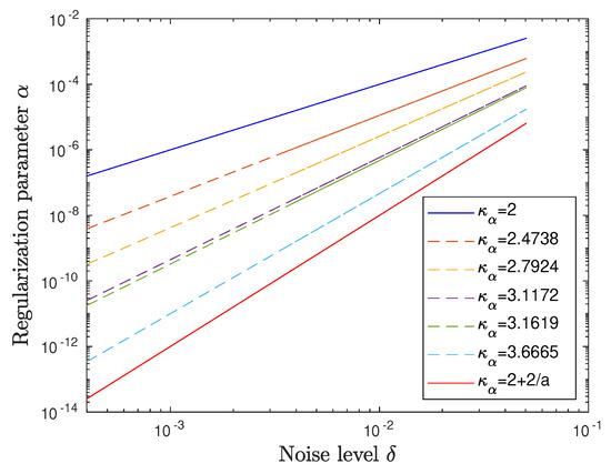
Figure 1. Regression lines for decay rates of ${\alpha }_{discr}$ for $\delta \to 0$ and different values $\beta$ from Table 1 on a double-logarithmic scale.

Figure 2 and Figure 3 give some more insight into the situation for the special case $\beta =0.2$, which approximately corresponds with the smoothness $x^{†}\in X_{0.31}$. In Figure 2 (left), the realized errors $\parallel x_{\alpha }^{\delta }-x^{†}{\parallel }_X$ are visualized for a discrete set of noise levels and compared with the associated regression line in a double-logarithmic scale. It becomes evident that the approximation using Hölder rates is highly accurate. The right image of Figure 2 visualizes the behavior of $\frac{{\delta }^2}{{\alpha }_{discr}}$ for various noise levels on a logarithmic scale. The tendency that $\frac{{\delta }^2}{{\alpha }_{discr}}\to \infty$ as $\delta \to 0$ seems to be convincing. Figure 3 (left) displays the realized ${\alpha }_{discr}$-values for this particular situation together with the best approximating regression line according to Equation (37). We see again a very good fit for this type of approximation. The right subfigure shows the exact and regularized solution for $\delta ={10}^{-3.5}$. The excellent fit of the regularized solution confirms our confidence in the numerical implementation, especially considering the problems associated with this type of exact solution.

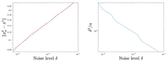
Figure 2. Approximation error $\parallel x_{\alpha }^{\delta }-x^{†}{\parallel }_X$ in red and approximate rate in blue/dashed (left) and $\frac{{\delta }^2}{{\alpha }_{discr}}$ (right), both depending on various $\delta$ on a log-log scale.

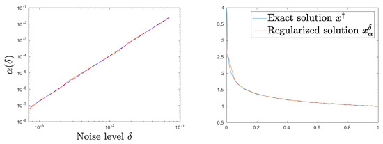
Figure 3. ${\alpha }_{discr}(\delta ,y^{\delta })$ in red for various $\delta$ and best approximating regression line in blue/dashed on a log-log scale (left). Regularized (red) compared with exact solution (blue) for $\delta ={10}^{-3.5}$ (right).

6.2. A Comparison with Results from A Priori Parameter Choices

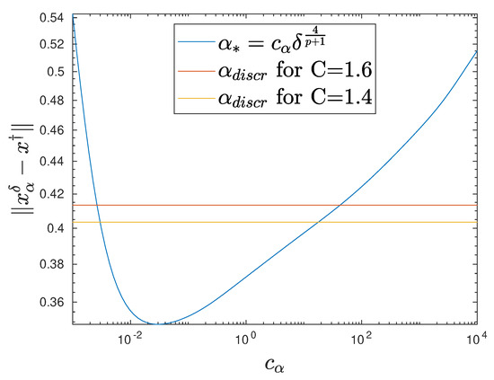
The question of whether the a posteriori choices using the discrepancy principle or appropriate a priori choices according to Equation (19) yield better results is of interest. The influence of the constant $c_{\alpha }$ when using a priori choice according to Equation (37) remains especially unclear. To numerically investigate this, we remain in the setting of Section 6.1; i.e., we consider $x^{†}\left(t\right)=c{t}^{-\beta }(0<t\le 1)$ as an exact solution. Figure 4 illuminates this situation for $\beta =0.2$. The error $\parallel x_{\alpha }^{\delta }-x^{†}{\parallel }_X$ is plotted for various constants $c_{\alpha }$, where we use ${\alpha }_{\ast }=\alpha \left(\delta \right)=c_{\alpha }{\delta }^{\frac{4}{1+p}}$. The error curve shows a clear minimum, which is connected with smaller values $\parallel x_{\alpha }^{\delta }-x^{†}{\parallel }_X$ compared with those obtained by exploiting the discrepancy principle with $C=1.4$ and $C=1.6$. It is completely unclear how to find suitable multipliers $c_{\alpha }$ in practice, whereas the discrepancy principle can always be applied as a robust parameter choice rule for practical applications.

Figure 4. Regularization error $\parallel x_{\alpha }^{\delta }-x^{†}{\parallel }_X$ using the a priori rate expressed in Equation (19) implemented in the sense of Equation (37) depending on various constants $c_{\alpha }$. Comparison with the error occurring for the discrepancy principle with C = 1.4 (orange) or C = 1.6 (red) and with noise level $\delta ={10}^{-2.5}$.

We complete our numerical experiments on a priori choices of the regularization parameter with Table 2 and Figure 5, where we list and illustrate the best regression exponents ${\kappa }_x$ according to the error norm estimate expressed in Equation (36) for different exponents ${\kappa }_{\alpha }$ in the a priori parameter choice expressed in Equation (37). In this case study, we used the exact solution $x\left(t\right)=1(0\le t\le 1)$ with the higher smoothness $p=0.5$. For the a priori parameter choice expressed in Equation (37) with varying exponents ${\kappa }_{\alpha }$, the factor $c_{\alpha }=1$ has been fixed. The discretization level $N=1000$ was considered.

Table 2. Error rates ${\kappa }_x$ by regression for $x^{†}\equiv 1$ and varying a priori exponents ${\kappa }_{\alpha }$.

a Priori $\mathit{\alpha }$-Rate ${\mathit{\kappa }}_{\mathit{\alpha }}$	2	2.5	2.66	3	3.5
convergence rate ${\kappa }_x$	0.2763	0.3304	0.3479	0.3686	0.3114

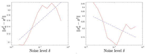
Figure 5. Regularization error $\parallel x_{\alpha }^{\delta }-x^{†}{\parallel }_X$ and regression line for different noise levels $\delta$ on a log-log scale. $x^{†}\left(t\right)=1$, a priori parameter choice according to Equation (37) with ${\kappa }_{\alpha }=3.5$ (left) and ${\kappa }_{\alpha }=5.5$ (right).

As expected, Table 2 indicates that maximal error rates occur if ${\kappa }_{\alpha }$ is close to the optimal value $\frac{4}{1+p}$. These rates also correspond with the order optimal rates according to Equation (20). For smaller exponents ${\kappa }_{\alpha }$, the error rates are falling, and for large exponents ${\kappa }_{\alpha }\ge 2+\frac{2}{a}=4$, the convergence seems to degenerate. This is visualized in Figure 5: For ${\kappa }_{\alpha }=3.5$, convergence still takes place, whereas for ${\kappa }_{\alpha }=5.5$ convergence cannot be observed anymore.

Remark 6.

As an alternative a posteriori approach for choosing the regularization parameter $\alpha$, one could also consider the balancing (Lepskiĭ) principle (cf., e.g., [27,28]). In [29], this principle is adapted to the Hilbert scale setting, but not with respect to oversmoothing penalties. In future work, we can discuss this missing facet and perform numerical experiments for the balancing principle in the case of oversmoothing penalties.

References

- Hofmann, B.; Scherzer, O. Factors influencing the ill-posedness of nonlinear problems. Inverse Probl. 1994, 10, 1277–1297. [Google Scholar] [CrossRef]
- Morozov, V.A. Methods for Solving Incorrectly Posed Problems; Springer: New York, NY, USA, 1984. [Google Scholar]
- Hofmann, B.; Mathé, P. Tikhonov regularization with oversmoothing penalty for non-linear ill-posed problems in Hilbert scales. Inverse Probl. 2018, 34, 015007. [Google Scholar] [CrossRef]
- Anzengruber, S.W.; Hofmann, B.; Mathé, P. Regularization properties of the sequential discrepancy principle for Tikhonov regularization in Banach spaces. Appl. Anal. 2014, 93, 1382–1400. [Google Scholar] [CrossRef]
- Anzengruber, S.W.; Ramlau, R. Morozov’s discrepancy principle for Tikhonov-type functionals with nonlinear operators. Inverse Probl. 2010, 26, 025001. [Google Scholar] [CrossRef]
- Hofmann, B.; Plato, R. Convergence results and low order rates for nonlinear Tikhonov regularization with oversmoothing penalty term. Electron. Trans. Numer. Anal. 2020, 93. [Google Scholar]
- Engl, H.W.; Hanke, M.; Neubauer, A. Regularization of Inverse Problems; Volume 375 of Mathematics and Its Applications; Kluwer Academic Publishers Group: Dordrecht, The Netherlands, 1996. [Google Scholar]
- Natterer, F. Error bounds for Tikhonov regularization in Hilbert scales. Appl. Anal. 1984, 18, 29–37. [Google Scholar] [CrossRef]
- Hofmann, B.; Mathé, P. A priori parameter choice in Tikhonov regularization with oversmoothing penalty for non-linear ill-posed problems. In Springer Proceedings in Mathematics & Statistics; Cheng, J., Lu, S., Yamamoto, M., Eds.; Springer: Singapore, Singapore, 2020; pp. 169–176. [Google Scholar]
- Gerth, D.; Hofmann, B.; Hofmann, C. Case studies and a pitfall for nonlinear variational regularization under conditional stability. In Springer Proceedings in Mathematics & Statistics; Cheng, J., Lu, S., Yamamoto, M., Eds.; Springer: Singapore, Singapore, 2020; pp. 177–203. [Google Scholar]
- Schuster, T.; Kaltenbacher, B.; Hofmann, B.; Kazimierski, K.S. Regularization Methods in Banach Spaces; Volume 10 of Radon Series on Computational and Applied Mathematics; Walter de Gruyter: Berlin, Germany; Boston, MA, USA, 2012. [Google Scholar]
- Scherzer, O.; Grasmair, M.; Grossauer, H.; Haltmeier, M.; Lenzen, F. Variational Methods in Imaging; Volume 167 of Applied Mathematical Sciences; Springer: New York, NY, USA, 2009. [Google Scholar]
- Tikhonov, A.N.; Leonov, A.S.; Yagola, A.G. Nonlinear Ill-Posed Problems; Chapman & Hall: London, UK; New York, NY, USA, 1998; Volume 1. [Google Scholar]
- Cheng, J.; Yamamoto, M. One new strategy for a priori choice of regularizing parameters in Tikhonov’s regularization. Inverse Probl. 2000, 16, L31–L38. [Google Scholar] [CrossRef]
- Egger, H.; Hofmann, B. Tikhonov regularization in Hilbert scales under conditional stability assumptions. Inverse Probl. 2018, 34, 115015. [Google Scholar] [CrossRef]
- Neubauer, A. Tikhonov regularization of nonlinear ill-posed problems in Hilbert scales. Appl. Anal. 1992, 46, 59–72. [Google Scholar] [CrossRef]
- Tautenhahn, U. On a general regularization scheme for nonlinear ill-posed problems II: Regularization in Hilbert scales. Inverse Probl. 1998, 14, 1607–1616. [Google Scholar] [CrossRef]
- Adams, R.A.; Fournier, J.F.J. Sobolev Spaces; Elsevier/Academic Press: Amsterdam, The Netherlands, 2003. [Google Scholar]
- Neubauer, A. When do Sobolev spaces form a Hilbert scale? Proc. Am. Math. Soc. 1988, 103, 557–562. [Google Scholar] [CrossRef]
- Gorenflo, R.; Yamamoto, M. Operator-theoretic treatment of linear Abel integral equations of first kind. Jpn. J. Ind. Appl. Math. 1999, 16, 137–161. [Google Scholar] [CrossRef]
- Gorenflo, R.; Luchko, Y.; Yamamoto, M. Time-fractional diffusion equation in the fractional Sobolev spaces. Fract. Calc. Appl. Anal. 2015, 18, 799–820. [Google Scholar] [CrossRef]
- Hofmann, B.; Kaltenbacher, B.; Resmerita, E. Lavrentiev’s regularization method in Hilbert spaces revisited. Inverse Probl. 2016, 10, 741–764. [Google Scholar] [CrossRef]
- Plato, R.; Hofmann, B.; Mathé, P. Optimal rates for Lavrentiev regularization with adjoint source conditions. Math. Comput. 2018, 87, 785–801. [Google Scholar] [CrossRef]
- Groetsch, C.W. Inverse Problems in the Mathematical Sciences. In Vieweg Mathematics for Scientists and Engineers; Vieweg+Teubner Verlag: Wiesbaden, Germany, 1993. [Google Scholar]
- Hofmann, B. A local stability analysis of nonlinear inverse problems. In Inverse Problems in Engineering—Theory and Practice; The American Society of Mechanical Engineers: New York, NY, USA, 1998; pp. 313–320. [Google Scholar]
- Fleischer, G.; Hofmann, B. On inversion rates for the autoconvolution equation. Inverse Probl. 1996, 12, 419–435. [Google Scholar] [CrossRef]
- Mathé, P. The Lepskiĭ principle revisited. Inverse Probl. 2006, 22, L11–L15. [Google Scholar] [CrossRef]
- Lu, S.; Pereverzev, S.V.; Ramlau, R. An analysis of Tikhonov regularization for nonlinear ill-posed problems under a general smoothness assumption. Inverse Probl. 2007, 23, 217–230. [Google Scholar] [CrossRef]
- Pricop-Jeckstadt, M. Nonlinear Tikhonov regularization in Hilbert scales with balancing principle tuning parameter in statistical inverse problems. Inverse Probl. Sci. Eng. 2019, 27, 205–236. [Google Scholar] [CrossRef]
© 2020 by the authors. Licensee MDPI, Basel, Switzerland. This article is an open access article distributed under the terms and conditions of the Creative Commons Attribution (CC BY) license (http://creativecommons.org/licenses/by/4.0/).