Novel Multiple Attribute Group Decision-Making Methods Based on Linguistic Intuitionistic Fuzzy Information

Abstract

As an effective technique to qualitatively depict assessment information, a linguistic intuitionistic fuzzy number (LIFN) is more appropriate to portray vagueness and indeterminacy in actual situations than intuitionistic fuzzy number (IFN). The prominent feature of a Muirhead mean (MM) operator is that it has the powerful ability to capture the correlations between any input-data and MM operator covers other common operators by assigning the different parameter vectors. In the article, we first analyze the limitations of the existing ranking approaches of LIFN and propose a novel ranking approach to surmount these limitations. Secondly, we propound several novel MM operators to fuse linguistic intuitionistic fuzzy (LIF) information, such as the LIF Muirhead mean (LIFMM) operator, the weighted LIF Muirhead mean (WLIFMM) operator and their dual operators, the LIFDMM operator and the WLIFDMM operator. Subsequently, we discuss several desirable properties along with exceptional cases of them. Moreover, two novel multiple attribute group decision-making approaches are developed based upon these operators. Ultimately, the effectuality and practicability of the propounded methods are validated through dealing with a global supplier selection issue, and the comparative analysis and the merits of the presented approaches are demonstrated by comparing them with existing approaches.

1. Introduction

Decision-making (DM) is one of the most vital and fundamental missions of management, and it is also an important activity for an organization to achieve its ultimate goal. Multiple attribute group decision-making (MAGDM) is a significant constituent of modern decision science domains, the essence of which is to select the optimal alternatives on the basis of the assessment information obtained from a group of experts in terms of several given attributes. MAGDM problems are ubiquitous in various aspects of human life and have been paid a growing amount of attention by many scholars and fruitful research achievements have been made in this area [1,2,3,4,5,6,7,8]. As a result of the vagueness and uncertainty of DM settings and the difference of diverse experts’ knowledge levels, how to accurately represent the attribute assessment information in vague and nondeterminate environments is one of the most arduous challenges in the course of DM. For this, Zadeh [9] originally presented the definition of fuzzy sets (FS). Thereafter, a large number of research achievements on FS have been acquired, such as fuzzy reasoning [10,11,12], fuzzy decision-making [13,14,15], fuzzy algebraic [16,17,18] and so on. However, one of the defects of FS is that it only models the membership degree (MD) of an element belonging to a given objective. In order to surmount the shortcoming, Atanassov [19] extended FS to propound the intuitionistic fuzzy set (IFS) theory by adding a nonmembership degree (NMD). Since its emergence, a multitude of researchers have turned their attention to it and have made outstanding achievements in theory and application. For instance, Xia et al. [20] propounded several generalized aggregation operators for integrating intuitionistic fuzzy information based upon Archimedean t-norm and s-norm. Chen et al. [21] extended the evidential reasoning methodology to intuitionistic fuzzy environments to propound a novel DM approach. Xu et al. [22] presented some mathematical programming methods for consistency and consensus and applied intuitionistic fuzzy preference relations to build a DM approach. Liu et al. [23] combined the evidential reasoning and dynamic intuitionistic fuzzy weighted geometric operator to construct a DM approach. Garg et al. [24] propounded an extended TOPSIS approach by synthesizing the exponential distance and set pair analysis theory to address DM problems with interval-valued intuitionistic fuzzy information. Liu et al. [25] developed several intuitionistic fuzzy partitioned Maclaurin symmetric mean (MSM) operators of IFN to fuse intuitionistic fuzzy information. Dogan et al. [26] combined the Analytic Hierarchy Process (AHP) and Technique for Order Preference by Similarity to an Ideal Solution (TOPSIS) methods to settle the problem of corridor selection for locating autonomous vehicles under interval-valued intuitionistic fuzzy settings. Gao et al. [27] presented a novel target threat assessment method based on a three-way decision theory to deal with intuitionistic fuzzy DM issues. For more investigation achievements of IFS the reader can refer to References [28,29,30,31,32,33,34,35,36,37,38,39].

Although FS and IFS have been widely applied to many DM issues, all these techniques of DM models take into account the evaluation information from a quantitative point of view. Owing to the complexity of the decision context and the fuzziness of a decision-maker’s (DM’s) cognition, evaluators often express their preference for information qualitatively. When an expert assesses an accident, she/he often uses several natural language words to express his/her judgment information. For instance, when a police officer assesses a transport accident based on some conditions, he or she may use several linguistic words such as “very serious”, “serious” and “not too serious” to evaluate the accident. It is evident that the linguistic expressions are more in line with the assessment thinking of DMs and are more easily provided than fuzzy numbers and IFN. In order to resolve this drawback, Zadeh [40,41,42] firstly propounded the concept of linguistic variables (LV) and further proposed linguistic assessment methodology. For conquering the limitation of information loss, Xu [43] extended the discrete linguistic term set (LTS) to continuous LTS. Based upon the LV and IFN, Chen et al. [44] propounded the notion of a linguistic intuitionistic fuzzy number, in which the MD and NMD of a LIFN are depicted through LV; satisfying the sum of them is less than or equal to the upper boundary of LTS. It is evident that the LIFN synthesizes the superiorities of IFN and LV, which has a more predominant capability to tackle fuzzy DM problems. Since its presentation, research on it has received more and more attention and a lot of achievements have been acquired. Chen et al. [44] propounded the several basis aggregation operators of LIFN such as weighted averaging, weighted geometric and hybrid operators. Li et al. [45] developed the subtraction and division of LIFN and presented an extended VIKOR approach based on the entropy measure. Liu and Qin [46] propounded several Maclaurin symmetric mean (MSM) operators for aggregating LIF information, which can take into consideration the correlation of input data. Zhang et al. [47] extended an outranking method with LIFNs and applied the approach to tackling the coal mine safety evaluation problem. Liu and Liu [48] proposed some scaled prioritized operators to fuse LIFNs and established a new decision model.

As an effective skill for fusing different kinds of assessment information, the aggregation operator has become an indispensable branch in the field of information fusion. It can fuse the assessment information provided by DMs into a collective or integrate all assessment information of every alternative into a single comprehensive value. Because it takes into account two hierarchies of problems, it involves the comprehensive value of evaluation information and the order relation of alternatives. Therefore, many research achievements on the aggregation operator have been made by various domain scholars. Classical aggregation operators like weighted average, weighted geometric and ordered weighted average operators have been widely applied to the procedure of information fusion. However, these operators can only be utilized to tackle situations in which the attributes are independent. For practical DM problems, DMs frequently take into account the relevance of diverse attributes during the course of information integration. To conquer this issue, several special aggregation functions such as Bonferroni mean (BM) operator [49,50,51], Heronian mean (HM) operator [52,53,54,55] and MSM operator [56,57] are proposed in order to consider the interrelation of different attributes. Aiming at the aforementioned operators, we find that the BM operator and HM operator have the same characteristics in that they can only capture the interrelationship between any two attributes but they fail to consider the correlation between multiple input arguments. As a well-known aggregation operator, the MM operator was originally proposed by Muirhead [58] in 1902 and it has the following distinctive advantages: (1) it can consider the interrelationships between multiple input arguments during the procedure of information aggregation; (2) it is a generalized operator because it can get the existing operators by assigning different parameter vectors; (3) the adjustable parameters make the information fusion procedure more flexible. Since its introduction, Liu and Li [59] have put forward the dual MM (DMM) operator and several MM operators to aggregate IFNs. Hong et al. [60] propounded a weighted dual MM operator under the hesitant fuzzy environment. Wang et al. [61] developed several novel MM operators to integrate q-rung orthopair fuzzy information. Liu and Teng [62] developed extended MM operators to a probabilistic linguistic context for establishing a linguistic DM approach. Liu et al. [63] presented some uncertain 2-tuple linguistic MM operators based on the extended 2-tuple linguistic model. Up to now, the MM operator has not been utilized to address the DM problems with the assessment information portrayed by LIFN.

In a complex decision environment, the correlations of diverse attributes always exist in real-life applications. For instance, when we assess the quality of a computer, the performance and software configuration of the computer have a certain internal relationship. Therefore, it is vital for evaluators to consider the correlations of the attributes to attain a reasonable decision result. Additionally, the assessment information provided by the evaluator in the form of IFN is sometimes difficult to acquire, but they can easily give their judgment by the linguistic variable, such as “good”, “bad” and so forth. Hence, it is necessary to propound a novel linguistic decision approach to take into account the interrelationships of diverse attributes when evaluators desire to obtain rational decision results. Based upon the aforementioned analyses, we can derive the following results: (1) the LIFN synthesize the advantage of IFN and LV, which can efficiently express qualitative assessment information in complex fuzzy environment; (2) MM operator can seize the correlations of multi-data through the parameter vector, and it is a universalization operator of several existing operators.

Based upon the above-mentioned analyses, it is meaningful and necessary to generalize MM operator to LIF environment to process DM problems with LIFN information. So we combine the LIFN with MM operator to propound several novel aggregation operators to resolve the actual decision problems that consider the correlations of attribute in the decision process. Meanwhile, we build up new decision approaches on the basis of these operators to make the decision procedure more general and flexible. Accordingly, the objectives and contributions of this study are displayed below:

• to develop a novel ranking method for LIFNs to eliminate the defects of existing methods;
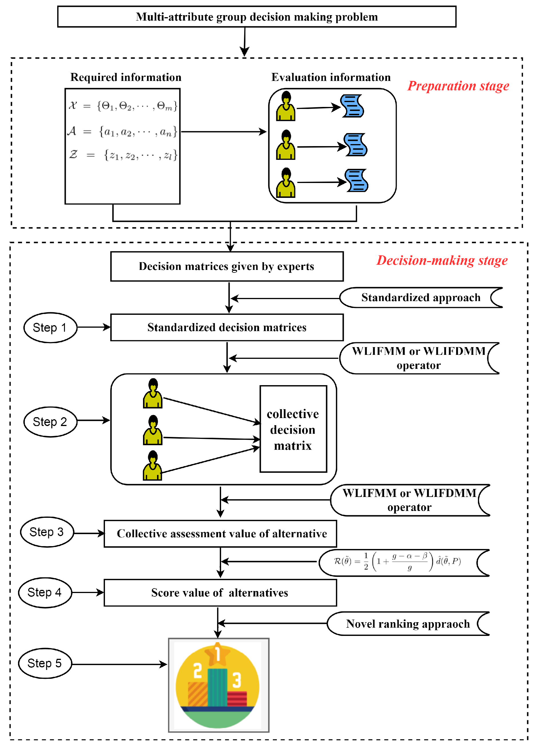
• to proffer several novel aggregation operators such as the LIFMM operator, the WLIFMM operator, the LIFDMM operator and the WLIFDMM operator.
• to study several paramount properties and particular instances of the developed operators;
• to propose two MAGDM approaches based upon the WLIFMM operator and the WLIFDMM operator;
• to demonstrate the significant merits of the presented methods through a comparative analysis and parameter analysis.

To accomplish the above objective, the surplus sections of this manuscript is allocated as below. Section 2 looks back on several fundamental notions of LIFN and MM operator. In Section 3, a novel comparison approach for LIFN is developed after analyzing the shortcomings of the existing ranking approach. In Section 4, the LIFMM operator, WLIFMM operator, LIFDMM operator and the WLIFDMM operator are developed and several properties and particular cases are discussed. In Section 5, two MAGDM approaches based on the WLIFMM operator and WLIFDMM operator are presented. In Section 6, a numerical example is given to demonstrate the availability and superiority of the presented method. Conclusively, several conclusions of this paper are given in the end.

2. Preliminaries

This part succinctly looks back on several fundamental concepts about LIFN and MM operator, which make readers easier to understand this research and lay a good foundation for the follow-up research.

2.1. LIFNs

The concept of LIFN firstly proposed by Chen et al. [44] in 2015, which is defined as below.

Definition 1

([44]). Assume that $\widehat{\mathcal{S}}=\left\{s_{\alpha }\right|\alpha \in [0,g]\}$ be a continuous linguistic terms set. For $s_{\alpha },s_{\beta }\in \widehat{\mathcal{S}}$, $\tilde{\theta }=(s_{\alpha },s_{\beta })$ is called a LIFN, if $\alpha +\beta \le g$. For simplicity, ${\overline{\mathsf{{\rm Y}}}}_{[0,g]}$ denotes the set of all LIFNs.

Remark 1.

Because $\alpha \in [0,g]$, then another expression of LIFN is shown as $\tilde{\theta }=(s_{\alpha },\mathrm{neg}\left(s_{\alpha }\right))$, where $\mathrm{neg}\left(s_{\alpha }\right)=s_{g-\alpha }$.

Definition 2

([44]). Assume that ${\tilde{\theta }}_i=(s_{{\alpha }_i},s_{{\beta }_i})(i=1,2)$$\in {\overline{\mathsf{{\rm Y}}}}_{[0,g]}$ with $\kappa >0$, then the operations of ${\tilde{\theta }}_1,{\tilde{\theta }}_2$ are shown as below.

1.

${\tilde{\theta }}_1\oplus {\tilde{\theta }}_2=\left(s_{{\alpha }_1+{\alpha }_2-\frac{{\alpha }_1{\alpha }_2}{g}},s_{\frac{{\beta }_1{\beta }_2}{g}}\right)$;

2.

${\tilde{\theta }}_1\otimes {\tilde{\theta }}_2=\left(s_{\frac{{\alpha }_1{\alpha }_2}{g}},s_{{\beta }_1+{\beta }_2-\frac{{\beta }_1{\beta }_2}{g}}\right)$;

3.

$\kappa {\tilde{\theta }}_1=\left(s_{g-g{(1-\frac{{\alpha }_1}{g})}^{\kappa }},s_{g{\left(\frac{{\beta }_1}{g}\right)}^{\kappa }}\right)$;

4.

${\tilde{\theta }}_1^{\kappa }=\left(s_{g{\left(\frac{{\alpha }_1}{g}\right)}^{\kappa }},s_{g-g{(1-\frac{{\beta }_1}{g})}^{\kappa }}\right)$.

Example 1.

Assume that ${\tilde{\theta }}_1=(s_4,s_3),{\tilde{\theta }}_2=(s_6,s_2)\in {\overline{\mathsf{{\rm Y}}}}_{[0,8]}$, with $\kappa =2$, then we have

1.

${\tilde{\theta }}_1\oplus {\tilde{\theta }}_2=\left(s_{4+6-\frac{4\times 6}{8}},s_{\frac{3\times 2}{8}}\right)=\left(s_7,s_{0.75}\right)$;

2.

${\tilde{\theta }}_1\otimes {\tilde{\theta }}_2=\left(s_{\frac{4\times 6}{8}},s_{3+2-\frac{3\times 2}{8}}\right)=\left(s_3,s_{4.25}\right)$;

3.

$2·{\tilde{\theta }}_1=\left(s_{8-8{(1-\frac{4}{8})}^2},s_{8{\left(\frac{3}{8}\right)}^2}\right)=\left(s_6,s_{1.125}\right)$;

4.

${\tilde{\theta }}_1^2=\left(s_{8{\left(\frac{4}{8}\right)}^2},s_{8-8{(1-\frac{3}{8})}^2}\right)=\left(s_2,s_{4.875}\right)$.

It is easy to prove the mentioned operational results are also LIFNs.

Theorem 1

([44]). Let ${\tilde{\theta }}_i=(s_{{\alpha }_i},s_{{\beta }_i})(i=1,2,3)$ be any three LIFNs and $\kappa ,{\kappa }_1,{\kappa }_2>0$, then

1.

${\tilde{\theta }}_1\oplus {\tilde{\theta }}_2={\tilde{\theta }}_2\oplus {\tilde{\theta }}_1$;

2.

${\tilde{\theta }}_1\otimes {\tilde{\theta }}_2={\tilde{\theta }}_2\otimes {\tilde{\theta }}_1$;

3.

${\tilde{\theta }}_1\oplus ({\tilde{\theta }}_2\oplus {\tilde{\theta }}_3)=({\tilde{\theta }}_1\oplus {\tilde{\theta }}_2)\oplus {\tilde{\theta }}_3$;

4.

${\tilde{\theta }}_1\otimes ({\tilde{\theta }}_2\oplus {\tilde{\theta }}_3)=({\tilde{\theta }}_1\otimes {\tilde{\theta }}_2)\oplus {\tilde{\theta }}_3$;

5.

$\kappa ({\tilde{\theta }}_1\oplus {\tilde{\theta }}_2)=k{\tilde{\theta }}_1\oplus \kappa {\tilde{\theta }}_2$;

6.

${({\tilde{\theta }}_1\otimes {\tilde{\theta }}_2)}^{\kappa }={\tilde{\theta }}_1^{\kappa }\otimes {\tilde{\theta }}_2^{\kappa }$;

7.

${\kappa }_1\tilde{\theta }\oplus {\kappa }_2\tilde{\theta }=({\kappa }_1+{\kappa }_2)\tilde{\theta }$;

8.

${\kappa }^{{\tilde{\theta }}_1}\otimes {\kappa }^{{\tilde{\theta }}_2}={\kappa }^{{\tilde{\theta }}_1+{\tilde{\theta }}_2}$;

9.

${\kappa }_1\left({\kappa }_2\tilde{\theta }\right)={\kappa }_1{\kappa }_2\tilde{\theta }$;

10.

${\left({\kappa }^{{\tilde{\theta }}_2}\right)}^{{\tilde{\theta }}_1}={\kappa }^{{\tilde{\theta }}_1{\tilde{\theta }}_2}$.

2.2. MM Operator

As a distinguished aggregation function, the notion of MM operator was originally propounded by Muirhead [58] in 1902.

Definition 3.

Suppose that ${\epsilon }_i(i=1,2,\dots ,n)$ is a group of positive numbers, $\mathcal{P}=(p_1,p_2,\dots ,p_n)\in {\mathbb{R}}^n$ is a parameters vector. The MM operators is expounded as:

$$\begin{array}{c}\hfill M{M}^{\mathcal{P}}\left({\epsilon }_1,{\epsilon }_2,\dots ,{\epsilon }_n\right)={\left(\frac{1}{n!}{\displaystyle \sum _{\xi \in S_n}}{\displaystyle \prod _{\tau =1}^n}{\epsilon }_{\xi \left(\tau \right)}^{p_{\tau }}\right)}^{\frac{1}{{\displaystyle \sum _{\tau =1}^n}{p}_{\tau }}},\end{array}$$

(1)

where $\xi \left(\tau \right)$ is denoted as any permutation of $(1,2,\dots ,n)$ and $S_n$ is the collection of all permutation of $(1,2,\dots ,n)$.

3. A Novel Ranking Approach of LIFN

The ultimate result of the DM problem is to pick the best alternative from a finite collection of alternatives. A reasonable comparison law is important for solving DM problems. In this section, we firstly analyze the shortcomings of the existing ranking approaches. Aiming at the analyzed shortcomings, a novel ranking approach for ranking LIFNs is presented to overcome the above defects.

Chen et al. [44] originally introduced the approach of ranking for LIFNs.

•   Ranking Approach I

Definition 4.

Let $\tilde{\theta }=(s_{\alpha },s_{\beta })$ be a LIFN, then the score function and accuracy function of $\tilde{\theta }$ are defined as below:

$$\begin{array}{cc}\hfill & \mathcal{LS}\left(\tilde{\theta }\right)=\alpha -\beta ;\hfill \\ \hfill & \mathcal{LH}\left(\tilde{\theta }\right)=\alpha +\beta .\hfill \end{array}$$

Based upon the score function and accuracy function of LIFN, the comparison method is defined as follows:

Definition 5.

Let ${\tilde{\theta }}_1=(s_{{\alpha }_1},s_{{\beta }_1}),{\tilde{\theta }}_2=(s_{{\alpha }_2},s_{{\beta }_2})\in {\overline{\mathsf{{\rm Y}}}}_{[0,t]}$. Then

1.

If $\mathcal{LS}\left({\tilde{\theta }}_1\right)<\mathcal{LS}\left({\tilde{\theta }}_2\right)$, then ${\tilde{\theta }}_1\prec {\tilde{\theta }}_2$;

2.

If $\mathcal{LS}\left({\tilde{\theta }}_1\right)=\mathcal{LS}\left({\tilde{\theta }}_2\right)$, then,

• If $\mathcal{LH}\left(\tilde{\theta }1\right)>\mathcal{LH}\left({\tilde{\theta }}_2\right)$, then ${\tilde{\theta }}_1\succ {\tilde{\theta }}_2$;
• If $\mathcal{LH}\left({\tilde{\theta }}_1\right)=\mathcal{LH}\left({\tilde{\theta }}_2\right)$, then ${\tilde{\theta }}_1\sim {\tilde{\theta }}_2$.

The aforementioned comparison approach has two shortcomings: (1) it must synthesize the $\mathcal{LS}$ and $\mathcal{LH}$ to rank LIFN; (2) it fails to take into consideration the indeterminacy index of LIFN, i.e., it can produce an unreasonable ranking result. In the following, we will illustrate the aforementioned drawbacks by utilizing an example from [44].

Example 2.

For ${\tilde{\theta }}_1=(s_5,s_3),{\tilde{\theta }}_2=(s_5,s_2),{\tilde{\theta }}_3=(s_4,s_1)\in {\overline{\mathsf{{\rm Y}}}}_{[0,8]}$, we can obtain that:

$$\begin{array}{cc}\hfill & \mathcal{LS}\left({\tilde{\theta }}_1\right)=2,\mathcal{LS}\left({\tilde{\theta }}_2\right)=3,\mathcal{LS}\left({\tilde{\theta }}_3\right)=3,\hfill \\ \hfill & \mathcal{LH}\left({\tilde{\theta }}_1\right)=8,\mathcal{LH}\left({\tilde{\theta }}_2\right)=7,\mathcal{LS}\left({\tilde{\theta }}_3\right)=5.\hfill \end{array}$$

By the Ranking approach I, we can acquire that ${\tilde{\theta }}_2>{\tilde{\theta }}_3>{\tilde{\theta }}_1$.

•   Ranking Approach II

In order to perfect the operational laws of LIFNs, Li et al. [45] presented the subtraction and division operations of LIFNs and given another approach to sort LIFNs.

Definition 6.

Let $\tilde{\theta }=(s_{\alpha },s_{\beta })$ be a LIFNs, then

$$\begin{array}{cc}\hfill & \mathcal{L}\left(\tilde{\theta }\right)=\frac{\alpha +t-\beta }{2};\hfill \\ \hfill & \mathcal{H}\left(\tilde{\theta }\right)=\frac{\alpha +\beta }{2}.\hfill \end{array}$$

Based on the Definition 6, the comparison method of LIFNs is defined as below:

Definition 7.

Let ${\tilde{\theta }}_1=(s_{{\alpha }_1},s_{{\beta }_1}),{\tilde{\theta }}_2=(s_{{\alpha }_2},s_{{\beta }_2})\in {\overline{\mathsf{{\rm Y}}}}_{[0,t]}$. Then,

1.

If $\mathcal{L}\left({\tilde{\theta }}_1\right)>\mathcal{L}\left({\tilde{\theta }}_2\right)$, then ${\tilde{\theta }}_1\succ {\tilde{\theta }}_2$;

2.

If $\mathcal{L}\left({\tilde{\theta }}_1\right)=\mathcal{L}\left({\tilde{\theta }}_2\right)$, then,

• If $\mathcal{H}\left({\tilde{\theta }}_1\right)<\mathcal{H}\left({\tilde{\theta }}_2\right)$, then ${\tilde{\theta }}_1\prec {\tilde{\theta }}_2$;
• If $\mathcal{H}\left({\tilde{\theta }}_1\right)=\mathcal{H}\left({\tilde{\theta }}_2\right)$, then ${\tilde{\theta }}_1\sim {\tilde{\theta }}_2$.

•   Ranking Approach III

The ranking result obtained by Ranking approach I in Example 1 is ${\tilde{\theta }}_2>{\tilde{\theta }}_3>{\tilde{\theta }}_1$, which need combine the $\mathcal{LS}$ and $\mathcal{LH}$ to sort LIFNs. Although we can obtain the final ranking result, the loss of consistency will be produced in the process of comparison. Furthermore, the ranking result of ${\tilde{\theta }}_1$ and ${\tilde{\theta }}_3$ is ${\tilde{\theta }}_1<{\tilde{\theta }}_3$. However, when we consider the consistency of information, we have ${\tilde{\theta }}_1>{\tilde{\theta }}_3$. In this situation, we draw a unreasonable ranking result between ${\tilde{\theta }}_1$ and ${\tilde{\theta }}_3$.

When we use Ranking approach II to solve Example 1, we have $\mathcal{L}\left({\tilde{\theta }}_1\right)=5,\mathcal{L}\left({\tilde{\theta }}_2\right)=5.5$. So the ranking result is ${\tilde{\theta }}_2>{\tilde{\theta }}_3>{\tilde{\theta }}_1$. Although this approach only uses the score function to obtain the ranking result, the inconsistency of information is also produced.

Accordingly, a better ranking approach needs to be investigated for ranking LIFNs. By the means of the academic think in [64], we present a novel ranking approach which synthetically takes into account the hesitancy degree and positive ideal solution of LIFN. The proposed ranking approach can conquer the aforementioned drawbacks in Ranking Approach I. In what follows, we first propound a novel distance called generalized LIF distance.

Definition 8.

Assume that ${\tilde{\theta }}_i=(s_{{\alpha }_i},s_{{\beta }_i})(i=1,2)$ be two LIFNs. The generalized LIF distance between ${\tilde{\theta }}_1$ and ${\tilde{\theta }}_2$ is elaborated as below:

$$\begin{array}{c}\hfill \widehat{d}({\tilde{\theta }}_1,{\tilde{\theta }}_2)={\left\{\frac{1}{2g}\left(|{\alpha }_1-{\alpha }_2{|}^{\chi }+|{\beta }_1-{\beta }_1{|}^{\chi }+{|{\pi }_1-{\pi }_2|}^{\chi }\right)\right\}}^{\frac{1}{\chi }},\end{array}$$

(2)

where ${\pi }_i=g-{\alpha }_i-{\beta }_i(i=1,2)$ and $\chi \ge 1$.

Several particular cases of the generalized LIF distance shall be given by assigning different values $\chi$.

Case 1.

When $\chi =1$, the generalized LIF distance will degenerate into the LIF Hamming distance,

$$\begin{array}{c}\hfill \widehat{d}({\tilde{\theta }}_1,{\tilde{\theta }}_2)=\frac{1}{2g}\left(|{\alpha }_1-{\alpha }_2|+|{\beta }_1-{\beta }_1|+|{\pi }_1-{\pi }_2|\right).\end{array}$$

(3)

Case 2.

When $\chi =2$, the generalized LIF distance will degenerate into the LIF Euclidean distance,

$$\begin{array}{c}\hfill \widehat{d}({\tilde{\theta }}_1,{\tilde{\theta }}_2)={\left\{\frac{1}{2g}\left(|{\alpha }_1-{\alpha }_2{|}^2+|{\beta }_1-{\beta }_1{|}^2+{|{\pi }_1-{\pi }_2|}^2\right)\right\}}^{\frac{1}{2}}.\end{array}$$

(4)

Theorem 2.

Let ${\tilde{\theta }}_1,{\tilde{\theta }}_2$ be two LIFNs. The generalized LIF distance meets the following properties;

(P1) ${\tilde{\theta }}_1={\tilde{\theta }}_2$ iff $\widehat{d}({\tilde{\theta }}_1,{\tilde{\theta }}_2)=0$;

(P2) $\widehat{d}({\tilde{\theta }}_1,{\tilde{\theta }}_2)=\widehat{d}({\tilde{\theta }}_2,{\tilde{\theta }}_1)$;

(P3) $0\le \widehat{d}({\tilde{\theta }}_1,{\tilde{\theta }}_2)\le 1$.

Proof. 

P1 and P2 are obvious. We only prove P3.

(P3) For two LIFNs ${\tilde{\theta }}_1$ and ${\tilde{\theta }}_2$, we have

$$\begin{array}{cc}\hfill \widehat{d}({\tilde{\theta }}_1,{\tilde{\theta }}_2)& ={\left\{\frac{1}{2g}\left(|{\alpha }_1-{\alpha }_2{|}^{\chi }+|{\beta }_1-{\beta }_2{|}^{\chi }+{|{\pi }_1-{\pi }_2|}^{\chi }\right)\right\}}^{\frac{1}{\chi }}\hfill \\ \hfill & ={\left\{\frac{1}{2g}\left(|{\alpha }_1-{\alpha }_2{|}^{\chi }+|{\beta }_1-{\beta }_2{|}^{\chi }+{|(g-{\alpha }_1-{\beta }_1)-(g-{\alpha }_2-{\beta }_2)|}^{\chi }\right)\right\}}^{\frac{1}{\chi }}\hfill \\ \hfill & ={\left\{\frac{1}{2g}\left(|{\alpha }_1-{\alpha }_2{|}^{\chi }+|{\beta }_1-{\beta }_2{|}^{\chi }+{\left|({\alpha }_2-{\alpha }_1+{\beta }_2-{\beta }_1)\right|}^{\chi }\right)\right\}}^{\frac{1}{\chi }}\hfill \\ \hfill & \le {\left\{\frac{1}{2g}\left(|{\alpha }_1-{\alpha }_2{|}^{\chi }+|{\beta }_1-{\beta }_2{|}^{\chi }+|{\alpha }_1-{\alpha }_2{|}^{\chi }+{|{\beta }_1-{\beta }_2|}^{\chi }\right)\right\}}^{\frac{1}{\chi }}\hfill \\ \hfill & ={\left\{\frac{1}{g}\left(|{\alpha }_1-{\alpha }_2{|}^{\chi }+{|{\beta }_1-{\beta }_2|}^{\chi }\right)\right\}}^{\frac{1}{\chi }}.\hfill \end{array}$$

 □

According to $0\le {\alpha }_i,{\beta }_i,{\pi }_i\le g$ and ${\alpha }_i+{\beta }_i+{\pi }_i=g(i=1,2)$.

It is calculated that

$$0\le |{\alpha }_1-{\alpha }_2{|}^{\chi }+{|{\beta }_1-{\beta }_2|}^{\chi }\le g.$$

Accordingly, we get

$$0\le \frac{1}{g}{\left\{|{\alpha }_1-{\alpha }_2{|}^{\chi }+{|{\beta }_1-{\beta }_2|}^{\chi }\right\}}^{\frac{1}{\chi }}\le 1.$$

Therefore, it is acquired that $0\le \widehat{d}({\tilde{\theta }}_1,{\tilde{\theta }}_2)\le 1$.

Now, we give the definition of novel ranking approach on the basis of the generalized LIF distance.

Definition 9.

Let $\tilde{\theta }=(s_{\alpha },s_{\beta })$ be a LIFN. $P=(s_g,s_0)$ is the positive ideal point. The ranking index $\mathcal{R}$ of $\tilde{\theta }$ is expressed as below.

$$\begin{array}{c}\hfill \mathcal{R}\left(\tilde{\theta }\right)=\frac{1}{2}\left(1+\frac{g-\alpha -\beta }{g}\right)\widehat{d}(\tilde{\theta },P),\end{array}$$

(5)

in which $\widehat{d}(\tilde{\theta },P)$ is the generalized LIF distance between $\tilde{\theta }$ and P.

It is easy to know that the small the distance from $\tilde{\theta }$ to P, the alternative is closer to the ideal point. Hence, we can know that the small the value of $\mathcal{R}\left(\tilde{\theta }\right)$, the better the alternative $\tilde{\theta }$.

Example 3.

Let ${\tilde{\theta }}_1=(s_5,s_3),{\tilde{\theta }}_2=(s_5,s_2),{\tilde{\theta }}_3=(s_4,s_1)\in {\overline{\mathsf{{\rm Y}}}}_{[0,8]}$, we have $\mathcal{R}\left({\tilde{\theta }}_1\right)=0.1875$, $\mathcal{R}\left({\tilde{\theta }}_2\right)=0.2109$, $\mathcal{R}\left({\tilde{\theta }}_3\right)=0.3438$. By the above Ranking approach 3, we can acquire a more reasonable result ${\tilde{\theta }}_1>{\tilde{\theta }}_2>{\tilde{\theta }}_3$.

Example 4.

Assume that ${\tilde{\theta }}_1=(s_5,s_3),{\tilde{\theta }}_2=(s_7,s_1),{\tilde{\theta }}_3=(s_2,s_6),{\tilde{\theta }}_4=(s_3,s_4)\in {\overline{\mathsf{{\rm Y}}}}_{[0,8]}$, we utilize the above Ranking approaches to obtain the ranking result, respectively:

(1) Utilize the Ranking approach I, we have $\mathcal{LS}\left({\tilde{\theta }}_1\right)=2,\mathcal{LS}\left({\tilde{\theta }}_2\right)=6,\mathcal{LS}\left({\tilde{\theta }}_3\right)=-4,\mathcal{LS}\left({\tilde{\theta }}_4\right)=-1$, hence, the ranking result is ${\tilde{\theta }}_2>{\tilde{\theta }}_1>{\tilde{\theta }}_4>{\tilde{\theta }}_3$.

(2) Utilize the Ranking approach II, we have $\mathcal{L}\left({\tilde{\theta }}_1\right)=5,\mathcal{L}\left({\tilde{\theta }}_2\right)=7,\mathcal{L}\left({\tilde{\theta }}_3\right)=2,\mathcal{L}\left({\tilde{\theta }}_4\right)=3.5$, hence, the ranking result is ${\tilde{\theta }}_2>{\tilde{\theta }}_1>{\tilde{\theta }}_4>{\tilde{\theta }}_3$.

(3) Utilize the Ranking approach III, when $\chi =3$, by utilizing the Comparison Approach III, the we have $\mathcal{R}\left({\tilde{\theta }}_1\right)=0.1181,\mathcal{R}\left({\tilde{\theta }}_2\right)=0.0394,\mathcal{R}\left({\tilde{\theta }}_3\right)=0.2362,\mathcal{R}\left({\tilde{\theta }}_4\right)=0.2021$, hence, the ranking result is ${\tilde{\theta }}_2>{\tilde{\theta }}_1>{\tilde{\theta }}_4>{\tilde{\theta }}_3$.

According to the above analysis and the utilization of Example 4, the proposed novel ranking approach has the following superiorities: (1) Compared with the score function proposed by [44,45], we can obtain that the final comparison result only need one step and it can reduce information loss; (2) The problem consistency of information is addressed valid; (3) The hesitation degree of DMs can be taken into consideration in the process of decision-making.

4. Linguistic Intuitionistic Fuzzy Muirhead Mean Operators

In this section, we shall develop some linguistic intuitionistic fuzzy Muirhead mean operators and explore some desirable properties of them.

4.1. Linguistic Intuitionistic Fuzzy Muirhead Mean Operator

Definition 10.

Assume that ${\tilde{\theta }}_i=(s_{{\alpha }_i},s_{{\beta }_i})(i=1,2,\dots ,n)$ be a set of LIFNs, and $\mathcal{P}=(p_1,p_2,\dots ,p_n)\in {\mathbb{R}}^n$ be a parameters vector, then the LIFMM operator is expressed as:

$$\begin{array}{c}\hfill LIFM{M}^{\mathcal{P}}\left({\tilde{\theta }}_1,{\tilde{\theta }}_2,\dots ,{\tilde{\theta }}_n\right)={\left(\frac{1}{n!}{\displaystyle \sum _{\xi \in S_n}}{\displaystyle \prod _{\tau =1}^n}{\tilde{\theta }}_{\xi \left(\tau \right)}^{p_{\tau }}\right)}^{\frac{1}{{\displaystyle \sum _{\tau =1}^n}{p}_{\tau }}},\end{array}$$

where $\xi \left(\tau \right)(\tau =1,2,\dots ,n)$ and $S_n$ is denoted any permutation and a collection of all permutation of $(1,2,\dots ,n)$, respectively.

Theorem 3.

Assume that ${\tilde{\theta }}_i=(s_{{\alpha }_i},s_{{\beta }_i})(i=1,2,\dots ,n)$ be a collection of LIFNs, then the fused result by LIFMM operators is also a LIFN, and it can be gained by

$$\begin{array}{c}LIFM{M}^{\mathcal{P}}\left({\tilde{\theta }}_1,{\tilde{\theta }}_2,\dots ,{\tilde{\theta }}_n\right)=\left(s_{g{\left(1-{\left({\displaystyle \prod _{\xi \in S_n}}\left(1-{\displaystyle \prod _{\tau =1}^n}{\left(\frac{{\alpha }_{\xi \left(\tau \right)}}{g}\right)}^{p_{\tau }}\right)\right)}^{\frac{1}{n!}}\right)}^{\frac{1}{{\displaystyle \sum _{\tau =1}^n}{p}_{\tau }}}},s_{g-g{\left(1-{\left({\displaystyle \prod _{\xi \in S_n}}\left(1-{\displaystyle \prod _{\tau =1}^n}{\left(1-\frac{{\beta }_{\xi \left(\tau \right)}}{g}\right)}^{p_{\tau }}\right)\right)}^{\frac{1}{n!}}\right)}^{\frac{1}{{\displaystyle \sum _{\tau =1}^n}{p}_{\tau }}}}\right).\end{array}$$

(6)

Proof. 

(1) We shall prove that the Equation (6) holds; (2) Equation (6) is an LIFN.

(1) According to the operational rules of LIFNs, we gain

$$\begin{array}{c}\hfill {\tilde{\theta }}_{\xi \left(\tau \right)}^{p_{\tau }}=\left(s_{g{\left(\frac{{\alpha }_{\xi \left(\tau \right)}}{g}\right)}^{p_{\tau }}},s_{g\left(1-{\left(1-\frac{{\beta }_{\xi \left(\tau \right)}}{g}\right)}^{p_{\tau }}\right)}\right)\end{array}$$

and

$$\begin{array}{c}\hfill {\displaystyle \prod _{\tau =1}^n}{\tilde{\theta }}_{\xi \left(\tau \right)}^{p_{\tau }}=\left(s_{g{\displaystyle \prod _{\tau =1}^n}{\left(\frac{{\alpha }_{\xi \left(\tau \right)}}{g}\right)}^{p_{\tau }}},s_{g\left(1-{\displaystyle \prod _{\tau =1}^n}{\left(1-\frac{{\beta }_{\xi \left(\tau \right)}}{g}\right)}^{p_{\tau }}\right)}\right).\end{array}$$

Then

$$\begin{array}{c}\hfill {\displaystyle \sum _{\xi \in S_n}}{\displaystyle \prod _{\tau =1}^n}{\tilde{\theta }}_{\xi \left(\tau \right)}^{p_{\tau }}=\left(s_{g\left(1-{\displaystyle \prod _{\xi \in S_n}}\left(1-{\displaystyle \prod _{\tau =1}^n}{\left(\frac{{\alpha }_{\xi \left(\tau \right)}}{g}\right)}^{p_{\tau }}\right)\right)},s_{g\left({\displaystyle \prod _{\xi \in S_n}}\left(1-{\displaystyle \prod _{\tau =1}^n}{\left(1-\frac{{\beta }_{\xi \left(\tau \right)}}{g}\right)}^{p_{\tau }}\right)\right)}\right).\end{array}$$

Further

$$\begin{array}{c}\hfill \frac{1}{n!}{\displaystyle \sum _{\xi \in S_n}}{\displaystyle \prod _{\tau =1}^n}{\tilde{\theta }}_{\xi \left(\tau \right)}^{p_{\tau }}=\left(s_{g{\left(1-{\displaystyle \prod _{\xi \in S_n}}\left(1-{\displaystyle \prod _{\tau =1}^n}{\left(\frac{{\alpha }_{\xi \left(\tau \right)}}{g}\right)}^{p_{\tau }}\right)\right)}^{\frac{1}{n!}}},s_{g\left({\displaystyle \prod _{\xi \in S_n}}{\left(1-{\displaystyle \prod _{\tau =1}^n}{\left(1-\frac{{\beta }_{\xi \left(\tau \right)}}{g}\right)}^{p_{\tau }}\right)}^{\frac{1}{n!}}\right)}\right).\end{array}$$

Hence, we get

$$\begin{array}{c}\hfill LIFM{M}^P\left({\tilde{\theta }}_1,{\tilde{\theta }}_2,\dots ,{\tilde{\theta }}_n\right)=\left(s_{g{\left(1-{\left({\displaystyle \prod _{\xi \in S_n}}\left(1-{\displaystyle \prod _{\tau =1}^n}{\left(\frac{{\alpha }_{\xi \left(\tau \right)}}{g}\right)}^{p_{\tau }}\right)\right)}^{\frac{1}{n!}}\right)}^{\frac{1}{{\displaystyle \sum _{\tau =1}^n}{p}_{\tau }}}},s_{g-g{\left(1-{\left({\displaystyle \prod _{\xi \in S_n}}\left(1-{\displaystyle \prod _{\tau =1}^n}{\left(1-\frac{{\beta }_{\xi \left(\tau \right)}}{g}\right)}^{p_{\tau }}\right)\right)}^{\frac{1}{n!}}\right)}^{\frac{1}{{\displaystyle \sum _{\tau =1}^n}{p}_{\tau }}}}\right).\end{array}$$

(2) In the following, we prove that Equation (6) is a LIFN. Suppose that

$$\begin{array}{cc}\hfill & \aleph =g{\left(1-{\left({\displaystyle \prod _{\xi \in S_n}}\left(1-{\displaystyle \prod _{\tau =1}^n}{\left(\frac{{\alpha }_{\xi \left(\tau \right)}}{g}\right)}^{p_{\tau }}\right)\right)}^{\frac{1}{n!}}\right)}^{\frac{1}{{\displaystyle \sum _{\tau =1}^n}{p}_{\tau }}},\hfill \\ \hfill & \hslash =g-g{\left(1-{\left({\displaystyle \prod _{\xi \in S_n}}\left(1-{\displaystyle \prod _{\tau =1}^n}{\left(1-\frac{{\beta }_{\xi \left(\tau \right)}}{g}\right)}^{p_{\tau }}\right)\right)}^{\frac{1}{n!}}\right)}^{\frac{1}{{\displaystyle \sum _{\tau =1}^n}{p}_{\tau }}}.\hfill \end{array}$$

Then, we need to prove that the listed conditions are kept.

(i) $0\le \aleph \le g,0\le \hslash \le g$;

(ii) $0\le \aleph +\hslash \le g$.

(i) Because ${\alpha }_{\xi \left(\tau \right)}\in [0,g]$, we can obtain

$$\begin{array}{cc}\hfill & {\displaystyle \prod _{\tau =1}^n}{\left(\frac{{\alpha }_{\xi \left(\tau \right)}}{g}\right)}^{p_{\tau }}\in [0,1]\Rightarrow 1-{\displaystyle \prod _{\tau =1}^n}{\left(\frac{{\alpha }_{\xi \left(\tau \right)}}{g}\right)}^{p_{\tau }}\in [0,1]\hfill \\ \hfill & \Rightarrow {\displaystyle \prod _{\xi \in S_n}}\left(1-{\displaystyle \prod _{\tau =1}^n}{\left(\frac{{\alpha }_{\xi \left(\tau \right)}}{g}\right)}^{p_{\tau }}\right)\in [0,1]\Rightarrow {\left({\displaystyle \prod _{\xi \in S_n}}\left(1-{\displaystyle \prod _{\tau =1}^n}{\left(\frac{{\alpha }_{\xi \left(\tau \right)}}{g}\right)}^{p_{\tau }}\right)\right)}^{\frac{1}{n!}}\in [0,1]\hfill \\ \hfill & \Rightarrow 1-{\left({\displaystyle \prod _{\xi \in S_n}}\left(1-{\displaystyle \prod _{\tau =1}^n}{\left(\frac{{\alpha }_{\xi \left(\tau \right)}}{g}\right)}^{p_{\tau }}\right)\right)}^{\frac{1}{n!}}\in [0,1]\Rightarrow {\left(1-{\left({\displaystyle \prod _{\xi \in S_n}}\left(1-{\displaystyle \prod _{\tau =1}^n}{\left(\frac{{\alpha }_{\xi \left(\tau \right)}}{g}\right)}^{p_{\tau }}\right)\right)}^{\frac{1}{n!}}\right)}^{\frac{1}{{\displaystyle \sum _{\tau =1}^n}{p}_{\tau }}}\in [0,1]\hfill \\ \hfill & \Rightarrow g{\left(1-{\left({\displaystyle \prod _{\xi \in S_n}}\left(1-{\displaystyle \prod _{\tau =1}^n}{\left(\frac{{\alpha }_{\xi \left(\tau \right)}}{g}\right)}^{p_{\tau }}\right)\right)}^{\frac{1}{n!}}\right)}^{\frac{1}{{\displaystyle \sum _{\tau =1}^n}{p}_{\tau }}}\in [0,g].\hfill \end{array}$$

Similarly, we can easily gain

$$\begin{array}{c}\hfill g-g{\left(1-{\left({\displaystyle \prod _{\xi \in S_n}}\left(1-{\displaystyle \prod _{\tau =1}^n}{\left(1-\frac{{\beta }_{\xi \left(\tau \right)}}{g}\right)}^{p_{\tau }}\right)\right)}^{\frac{1}{n!}}\right)}^{\frac{1}{{\displaystyle \sum _{\tau =1}^n}{p}_{\tau }}}\in [0,g].\end{array}$$

Hence, the condition (i) is satisfied.

(ii) Since $0\le {\alpha }_{\xi \left(\tau \right)}+{\beta }_{\xi \left(\tau \right)}\le g$, then ${\alpha }_{\xi \left(\tau \right)}\le g-{\beta }_{\xi \left(\tau \right)}$. Then

$$\begin{array}{c}\aleph +\hslash =g{\left(1-{\left({\displaystyle \prod _{\xi \in S_n}}\left(1-{\displaystyle \prod _{\tau =1}^n}{\left(\frac{{\alpha }_{\xi \left(\tau \right)}}{g}\right)}^{p_{\tau }}\right)\right)}^{\frac{1}{n!}}\right)}^{\frac{1}{{\displaystyle \sum _{\tau =1}^n}{p}_{\tau }}}+g-g{\left(1-{\left({\displaystyle \prod _{\xi \in S_n}}\left(1-{\displaystyle \prod _{\tau =1}^n}{\left(1-\frac{{\beta }_{\xi \left(\tau \right)}}{g}\right)}^{p_{\tau }}\right)\right)}^{\frac{1}{n!}}\right)}^{\frac{1}{{\displaystyle \sum _{\tau =1}^n}{p}_{\tau }}}\\ \le g{\left(1-{\left({\displaystyle \prod _{\xi \in S_n}}\left(1-{\displaystyle \prod _{\tau =1}^n}{\left(\frac{g-{\beta }_{\xi \left(\tau \right)}}{g}\right)}^{p_{\tau }}\right)\right)}^{\frac{1}{n!}}\right)}^{\frac{1}{{\displaystyle \sum _{\tau =1}^n}{p}_{\tau }}}+g-g{\left(1-{\left({\displaystyle \prod _{\xi \in S_n}}\left(1-{\displaystyle \prod _{\tau =1}^n}{\left(1-\frac{{\beta }_{\xi \left(\tau \right)}}{g}\right)}^{p_{\tau }}\right)\right)}^{\frac{1}{n!}}\right)}^{\frac{1}{{\displaystyle \sum _{\tau =1}^n}{p}_{\tau }}}=g.\end{array}$$

(7)

Hence, We obtain $0\le \aleph +\hslash \le g.$

It is evident that the fused value by the LIFMM operator is still an LIFN. Accordingly, Theorem 2 is proved by analyzing (1) and (2). □

In the next, we shall investigate several anticipated properties of LIFMM operator.

Theorem 4

(Idempotency). If ${\tilde{\theta }}_i=(s_{{\alpha }_i},s_{{\beta }_i})(i=1,2,\dots ,n)$ are equal to $\tilde{\theta }=(s_{\alpha },s_{\beta })$, then

$$\begin{array}{c}\hfill LIFM{M}^{\mathcal{P}}\left({\tilde{\theta }}_1,{\tilde{\theta }}_2,\dots ,{\tilde{\theta }}_n\right)=\tilde{\theta }.\end{array}$$

(8)

Proof. 

Since ${\tilde{\theta }}_i=\tilde{\theta }=(s_{\alpha },s_{\beta })$, we have

$$\begin{array}{cc}\hfill LIFM{M}^g\left({\tilde{\theta }}_1,{\tilde{\theta }}_2,\dots ,{\tilde{\theta }}_n\right)& =\left(s_{g{\left(1-{\left({\displaystyle \prod _{\xi \in S_n}}\left(1-{\displaystyle \prod _{\tau =1}^n}{\left(\frac{{\alpha }_{\xi \left(\tau \right)}}{g}\right)}^{p_{\tau }}\right)\right)}^{\frac{1}{n!}}\right)}^{\frac{1}{{\displaystyle \sum _{\tau =1}^n}{p}_{\tau }}}},s_{g-g{\left(1-{\left({\displaystyle \prod _{\xi \in S_n}}\left(1-{\displaystyle \prod _{\tau =1}^n}{\left(1-\frac{{\beta }_{\xi \left(\tau \right)}}{g}\right)}^{p_{\tau }}\right)\right)}^{\frac{1}{n!}}\right)}^{\frac{1}{{\displaystyle \sum _{\tau =1}^n}{p}_{\tau }}}}\right)\hfill \\ \hfill & =\left(s_{g{\left(1-{\left({\left(1-{\left(\frac{\alpha }{g}\right)}^{{\displaystyle \sum _{\tau =1}^n}{p}_{\tau }}\right)}^{n!}\right)}^{\frac{1}{n!}}\right)}^{\frac{1}{{\displaystyle \sum _{\tau =1}^n}{p}_{\tau }}}},s_{g-g{\left(1-{\left({\left(1-{\left(1-\frac{\beta }{g}\right)}^{{\displaystyle \sum _{\tau =1}^n}{p}_{\tau }}\right)}^{n!}\right)}^{\frac{1}{n!}}\right)}^{\frac{1}{{\displaystyle \sum _{\tau =1}^n}{p}_{\tau }}}}\right)\hfill \\ \hfill & =\left(s_{g{\left(1-\left(1-{\left(\frac{\alpha }{g}\right)}^{{\displaystyle \sum _{\tau =1}^n}{p}_{\tau }}\right)\right)}^{\frac{1}{{\displaystyle \sum _{\tau =1}^n}{p}_{\tau }}}},s_{g-g{\left(1-\left(1-{\left(1-\frac{\beta }{g}\right)}^{{\displaystyle \sum _{\tau =1}^n}{p}_{\tau }}\right)\right)}^{\frac{1}{{\displaystyle \sum _{\tau =1}^n}{p}_{\tau }}}}\right)\hfill \\ \hfill & =\left(s_{g{\left({\left(\frac{\alpha }{g}\right)}^{{\displaystyle \sum _{\tau =1}^n}{p}_{\tau }}\right)}^{\frac{1}{{\displaystyle \sum _{\tau =1}^n}{p}_{\tau }}}},s_{g-g{\left({\left(1-\frac{\beta }{g}\right)}^{{\displaystyle \sum _{\tau =1}^n}{p}_{\tau }}\right)}^{\frac{1}{{\displaystyle \sum _{\tau =1}^n}{p}_{\tau }}}}\right)\hfill \\ \hfill & =\left(s_{g\left(\frac{\alpha }{g}\right)},s_{g-g\left(1-\frac{\beta }{g}\right)}\right)=(s_{\alpha },s_{\beta })=\tilde{\theta }\hfill \end{array}$$

 □

Theorem 5

(Monotonicity). Let ${\tilde{\theta }}_i=(s_{{\alpha }_i},s_{{\beta }_i})$ and ${\tilde{\theta }}_i^{{}^{\prime }}=(s_{{\alpha }_i^{{}^{\prime }}},s_{{\beta }_i^{{}^{\prime }}})$ be two collections of LIFNs. If, $s_{{\alpha }_i}\ge s_{{\alpha }_i^{{}^{\prime }}},s_{{\beta }_i}\le s_{{\beta }_i^{{}^{\prime }}}$ for each i. Then

$$\begin{array}{c}\hfill LIFM{M}^{\mathcal{P}}\left({\tilde{\theta }}_1,{\tilde{\theta }}_2,\dots ,{\tilde{\theta }}_n\right)\ge LIFM{M}^{\mathcal{P}}\left({\tilde{\theta }}_1^{{}^{\prime }},{\tilde{\theta }}_2^{{}^{\prime }},\dots ,{\tilde{\theta }}_n^{{}^{\prime }}\right).\end{array}$$

(9)

Proof. 

Since $s_{{\alpha }_i}\ge s_{{\alpha }_i^{{}^{\prime }}}\ge 0$, $s_{{\beta }_i^{{}^{\prime }}}\ge s_{{\beta }_i}\ge 0$, we have ${\alpha }_i\ge {\alpha }_i^{{}^{\prime }},{\beta }_i\le {\beta }_i^{{}^{\prime }}$, then

$$\begin{array}{cc}\hfill & \frac{{\alpha }_{\xi \left(\tau \right)}}{g}\ge \frac{{\alpha }_{\xi \left(\tau \right)}^{{}^{\prime }}}{g}\Rightarrow {\displaystyle \prod _{\tau =1}^n}{\left(\frac{{\alpha }_{\xi \left(\tau \right)}}{g}\right)}^{p_{\tau }}\ge {\displaystyle \prod _{\tau =1}^n}{\left(\frac{{\alpha }_{\xi \left(\tau \right)}^{{}^{\prime }}}{g}\right)}^{p_{\tau }}\hfill \\ \hfill & \Rightarrow {\displaystyle \prod _{\xi \in S_n}}\left(1-{\displaystyle \prod _{\tau =1}^n}{\left(\frac{{\alpha }_{\xi \left(\tau \right)}}{g}\right)}^{p_{\tau }}\right)\le {\displaystyle \prod _{\xi \in S_n}}\left(1-{\displaystyle \prod _{\tau =1}^n}{\left(\frac{{\alpha }_{\xi \left(\tau \right)}^{{}^{\prime }}}{g}\right)}^{p_{\tau }}\right)\hfill \\ \hfill & \Rightarrow 1-{\left({\displaystyle \prod _{\xi \in S_n}}\left(1-{\displaystyle \prod _{\tau =1}^n}{\left(\frac{{\alpha }_{\xi \left(\tau \right)}}{g}\right)}^{p_{\tau }}\right)\right)}^{\frac{1}{n!}}\ge 1-{\left({\displaystyle \prod _{\xi \in S_n}}\left(1-{\displaystyle \prod _{\tau =1}^n}{\left(\frac{{\alpha }_{\xi \left(\tau \right)}^{{}^{\prime }}}{g}\right)}^{p_{\tau }}\right)\right)}^{\frac{1}{n!}}\hfill \\ \hfill & \Rightarrow g{\left(1-{\left({\displaystyle \prod _{\xi \in S_n}}\left(1-{\displaystyle \prod _{\tau =1}^n}{\left(\frac{{\alpha }_{\xi \left(\tau \right)}}{g}\right)}^{p_{\tau }}\right)\right)}^{\frac{1}{n!}}\right)}^{\frac{1}{{\displaystyle \sum _{\tau =1}^n}{p}_{\tau }}}\ge g{\left(1-{\left({\displaystyle \prod _{\xi \in S_n}}\left(1-{\displaystyle \prod _{\tau =1}^n}{\left(\frac{{\alpha }_{\xi \left(\tau \right)}^{{}^{\prime }}}{g}\right)}^{p_{\tau }}\right)\right)}^{\frac{1}{n!}}\right)}^{\frac{1}{{\displaystyle \sum _{\tau =1}^n}{p}_{\tau }}}\hfill \end{array}$$

Similarly, we have

$$\begin{array}{c}\frac{{\beta }_{\xi \left(\tau \right)}}{g}\le \frac{{\beta }_{\xi \left(\tau \right)}^{{}^{\prime }}}{g}\Rightarrow {\displaystyle \prod _{\tau =1}^n}{\left(1-\frac{{\beta }_{\xi \left(\tau \right)}}{g}\right)}^{p_{\tau }}\ge {\displaystyle \prod _{\tau =1}^n}{\left(1-\frac{{\beta }_{\xi \left(\tau \right)}^{{}^{\prime }}}{g}\right)}^{p_{\tau }}\hfill \\ \Rightarrow {\displaystyle \prod _{\xi \in S_n}}\left(1-{\displaystyle \prod _{\tau =1}^n}{\left(1-\frac{{\beta }_{\xi \left(\tau \right)}}{g}\right)}^{p_{\tau }}\right)\le {\displaystyle \prod _{\xi \in S_n}}\left(1-{\displaystyle \prod _{\tau =1}^n}{\left(1-\frac{{\beta }_{\xi \left(\tau \right)}^{{}^{\prime }}}{g}\right)}^{p_{\tau }}\right)\hfill \\ \Rightarrow {\left({\displaystyle \prod _{\xi \in S_n}}\left(1-{\displaystyle \prod _{\tau =1}^n}{\left(1-\frac{{\beta }_{\xi \left(\tau \right)}}{g}\right)}^{p_{\tau }}\right)\right)}^{\frac{1}{n!}}\le {\left({\displaystyle \prod _{\xi \in S_n}}\left(1-{\displaystyle \prod _{\tau =1}^n}{\left(1-\frac{{\beta }_{\xi \left(\tau \right)}^{{}^{\prime }}}{g}\right)}^{p_{\tau }}\right)\right)}^{\frac{1}{n!}}\hfill \\ \Rightarrow {\left(1-{\left({\displaystyle \prod _{\xi \in S_n}}\left(1-{\displaystyle \prod _{\tau =1}^n}{\left(1-\frac{{\beta }_{\xi \left(\tau \right)}}{g}\right)}^{p_{\tau }}\right)\right)}^{\frac{1}{n!}}\right)}^{\frac{1}{{\displaystyle \sum _{\tau =1}^n}{p}_{\tau }}}\ge {\left(1-{\left({\displaystyle \prod _{\xi \in S_n}}\left(1-{\displaystyle \prod _{\tau =1}^n}{\left(1-\frac{{\beta }_{\xi \left(\tau \right)}^{{}^{\prime }}}{g}\right)}^{p_{\tau }}\right)\right)}^{\frac{1}{n!}}\right)}^{\frac{1}{{\displaystyle \sum _{\tau =1}^n}{p}_{\tau }}}\hfill \\ \Rightarrow g-g{\left(1-{\left({\displaystyle \prod _{\xi \in S_n}}\left(1-{\displaystyle \prod _{\tau =1}^n}{\left(1-\frac{{\beta }_{\xi \left(\tau \right)}}{g}\right)}^{p_{\tau }}\right)\right)}^{\frac{1}{n!}}\right)}^{\frac{1}{{\displaystyle \sum _{\tau =1}^n}{p}_{\tau }}}\le g-g{\left(1-{\left({\displaystyle \prod _{\xi \in S_n}}\left(1-{\displaystyle \prod _{\tau =1}^n}{\left(1-\frac{{\beta }_{\xi \left(\tau \right)}^{{}^{\prime }}}{g}\right)}^{p_{\tau }}\right)\right)}^{\frac{1}{n!}}\right)}^{\frac{1}{{\displaystyle \sum _{\tau =1}^n}{p}_{\tau }}}\hfill \end{array}$$

(10)

Let $\mathcal{LS}\left(\tilde{\theta }\right),\mathcal{LS}\left({\tilde{\theta }}^{{}^{\prime }}\right)$ be the score values of $\tilde{\theta }$ and ${\tilde{\theta }}^{{}^{\prime }}$, respectively, where $\tilde{\theta }=LIFM{M}^{\mathcal{P}}\left({\tilde{\theta }}_1,{\tilde{\theta }}_2,\dots ,{\tilde{\theta }}_n\right),{\tilde{\theta }}^{{}^{\prime }}=LIFM{M}^{\mathcal{P}}\left({\tilde{\theta }}_1^{{}^{\prime }},{\tilde{\theta }}_2^{{}^{\prime }},\dots ,{\tilde{\theta }}_n^{{}^{\prime }}\right)$, respectively. Based on the score function of LIFNs and the aforementioned inequality, we can attain that $\mathcal{LS}\left(\tilde{\theta }\right)\ge \mathcal{LS}\left({\tilde{\theta }}^{{}^{\prime }}\right)$, then we discuss the following cases:

(i) If $\mathcal{LS}\left(\tilde{\theta }\right)>\mathcal{LS}\left({\tilde{\theta }}^{{}^{\prime }}\right)$, then we can imply that

$$\begin{array}{c}\hfill LIFM{M}^{\mathcal{P}}\left({\tilde{\theta }}_1,{\tilde{\theta }}_2,\dots ,{\tilde{\theta }}_n\right)>LIFM{M}^{\mathcal{P}}\left({\tilde{\theta }}_1^{{}^{\prime }},{\tilde{\theta }}_2^{{}^{\prime }},\dots ,{\tilde{\theta }}_n^{{}^{\prime }}\right)\end{array}$$

(ii) If $\mathcal{LS}\left(\tilde{\theta }\right)=\mathcal{LS}\left({\tilde{\theta }}^{{}^{\prime }}\right)$, then

$$\begin{array}{cc}\hfill & g{\left(1-{\left({\displaystyle \prod _{\xi \in S_n}}\left(1-{\displaystyle \prod _{\tau =1}^n}{\left(\frac{{\alpha }_{\xi \left(\tau \right)}}{g}\right)}^{p_{\tau }}\right)\right)}^{\frac{1}{n!}}\right)}^{\frac{1}{{\displaystyle \sum _{\tau =1}^n}{p}_{\tau }}}-\left(g-g{\left(1-{\left({\displaystyle \prod _{\xi \in S_n}}\left(1-{\displaystyle \prod _{\tau =1}^n}{\left(1-\frac{{\beta }_{\xi \left(\tau \right)}}{g}\right)}^{p_{\tau }}\right)\right)}^{\frac{1}{n!}}\right)}^{\frac{1}{{\displaystyle \sum _{\tau =1}^n}{p}_{\tau }}}\right)\hfill \\ \hfill & =g{\left(1-{\left({\displaystyle \prod _{\xi \in S_n}}\left(1-{\displaystyle \prod _{\tau =1}^n}{\left(\frac{{\alpha }_{\xi \left(\tau \right)}}{g}\right)}^{p_{\tau }}\right)\right)}^{\frac{1}{n!}}\right)}^{\frac{1}{{\displaystyle \sum _{\tau =1}^n}{p}_{\tau }}}-\left(g-g{\left(1-{\left({\displaystyle \prod _{\xi \in S_n}}\left(1-{\displaystyle \prod _{\tau =1}^n}{\left(1-\frac{{\beta }_{\xi \left(\tau \right)}}{g}\right)}^{p_{\tau }}\right)\right)}^{\frac{1}{n!}}\right)}^{\frac{1}{{\displaystyle \sum _{\tau =1}^n}{p}_{\tau }}}\right)\hfill \end{array}$$

Since ${\alpha }_i\ge {\alpha }_i^{{}^{\prime }},{\beta }_i\le {\beta }_i^{{}^{\prime }}$ ,then based Definition 4, we can derive that

$$\begin{array}{c}\hfill g{\left(1-{\left({\displaystyle \prod _{\xi \in S_n}}\left(1-{\displaystyle \prod _{\tau =1}^n}{\left(\frac{{\alpha }_{\xi \left(\tau \right)}}{g}\right)}^{p_{\tau }}\right)\right)}^{\frac{1}{n!}}\right)}^{\frac{1}{{\displaystyle \sum _{\tau =1}^n}{p}_{\tau }}}=g{\left(1-{\left({\displaystyle \prod _{\xi \in S_n}}\left(1-{\displaystyle \prod _{\tau =1}^n}{\left(\frac{{\alpha }_{\xi \left(\tau \right)}^{{}^{\prime }}}{g}\right)}^{p_{\tau }}\right)\right)}^{\frac{1}{n!}}\right)}^{\frac{1}{{\displaystyle \sum _{\tau =1}^n}{p}_{\tau }}}\end{array}$$

and

$$\begin{array}{c}\hfill g-g{\left(1-{\left({\displaystyle \prod _{\xi \in S_n}}\left(1-{\displaystyle \prod _{\tau =1}^n}{\left(1-\frac{{\beta }_{\xi \left(\tau \right)}}{g}\right)}^{p_{\tau }}\right)\right)}^{\frac{1}{n!}}\right)}^{\frac{1}{{\displaystyle \sum _{\tau =1}^n}{p}_{\tau }}}=g-g{\left(1-{\left({\displaystyle \prod _{\xi \in S_n}}\left(1-{\displaystyle \prod _{\tau =1}^n}{\left(1-\frac{{\beta }_{\xi \left(\tau \right)}^{{}^{\prime }}}{g}\right)}^{p_{\tau }}\right)\right)}^{\frac{1}{n!}}\right)}^{\frac{1}{{\displaystyle \sum _{\tau =1}^n}{p}_{\tau }}}\end{array}$$

So, we can obtain that

$$\begin{array}{cc}\hfill & \mathcal{LH}\left(\tilde{\theta }\right)=g{\left(1-{\left({\displaystyle \prod _{\xi \in S_n}}\left(1-{\displaystyle \prod _{\tau =1}^n}{\left(\frac{{\alpha }_{\xi \left(\tau \right)}}{g}\right)}^{p_{\tau }}\right)\right)}^{\frac{1}{n!}}\right)}^{\frac{1}{{\displaystyle \sum _{\tau =1}^n}{p}_{\tau }}}+g-g{\left(1-{\left({\displaystyle \prod _{\xi \in S_n}}\left(1-{\displaystyle \prod _{\tau =1}^n}{\left(1-\frac{{\beta }_{\xi \left(\tau \right)}}{g}\right)}^{p_{\tau }}\right)\right)}^{\frac{1}{n!}}\right)}^{\frac{1}{{\displaystyle \sum _{\tau =1}^n}{p}_{\tau }}}\hfill \\ \hfill & =g{\left(1-{\left({\displaystyle \prod _{\xi \in S_n}}\left(1-{\displaystyle \prod _{\tau =1}^n}{\left(\frac{{\alpha }_{\xi \left(\tau \right)}^{{}^{\prime }}}{g}\right)}^{p_{\tau }}\right)\right)}^{\frac{1}{n!}}\right)}^{\frac{1}{{\displaystyle \sum _{\tau =1}^n}{p}_{\tau }}}+g-g{\left(1-{\left({\displaystyle \prod _{\xi \in S_n}}\left(1-{\displaystyle \prod _{\tau =1}^n}{\left(1-\frac{{\beta }_{\xi \left(\tau \right)}^{{}^{\prime }}}{g}\right)}^{p_{\tau }}\right)\right)}^{\frac{1}{n!}}\right)}^{\frac{1}{{\displaystyle \sum _{\tau =1}^n}{p}_{\tau }}}=\mathcal{LH}\left({\tilde{\theta }}^{{}^{\prime }}\right)\hfill \end{array}$$

Then, $LIFM{M}^{\mathcal{P}}\left({\tilde{\theta }}_1,{\tilde{\theta }}_2,\dots ,{\tilde{\theta }}_n\right)=LIFM{M}^{\mathcal{P}}\left({\tilde{\theta }}_1^{{}^{\prime }},{\tilde{\theta }}_2^{{}^{\prime }},\dots ,{\tilde{\theta }}_n^{{}^{\prime }}\right)$. □

Theorem 6

(Boundedness). Let ${\tilde{\theta }}_i=(s_{{\alpha }_i},s_{{\beta }_i})$ be a group of LIFNs, and ${\tilde{\theta }}^{-}=(s_{min\left({\alpha }_i\right)},s_{max\left({\beta }_i\right)})$, ${\tilde{\theta }}^{+}=(s_{max\left({\alpha }_i\right)},s_{min\left({\beta }_i\right)})$, then we can obtain

$$\begin{array}{c}\hfill {\tilde{\theta }}^{-}\le LIFM{M}^{\mathcal{P}}\left({\tilde{\theta }}_1,{\tilde{\theta }}_2,\dots ,{\tilde{\theta }}_n\right)\le {\tilde{\theta }}^{+}.\end{array}$$

(11)

Proof. 

On the basis of Theorem 4 and 5, we can get

$$\begin{array}{c}\hfill LIFM{M}^{\mathcal{P}}\left({\tilde{\theta }}_1,{\tilde{\theta }}_2,\dots ,{\tilde{\theta }}_n\right)\ge LIFM{M}^{\mathcal{P}}\left({\tilde{\theta }}^{-},{\tilde{\theta }}^{-},\dots ,{\tilde{\theta }}^{-}\right)={\tilde{\theta }}^{-}\end{array}$$

and

$$\begin{array}{c}\hfill LIFM{M}^{\mathcal{P}}\left({\tilde{\theta }}_1,{\tilde{\theta }}_2,\dots ,{\tilde{\theta }}_n\right)\le LIFM{M}^{\mathcal{P}}\left({\tilde{\theta }}^{+},{\tilde{\theta }}^{+},\dots ,{\tilde{\theta }}^{+}\right)={\tilde{\theta }}^{+}.\end{array}$$

So, we have

$$\begin{array}{c}\hfill {\theta }^{-}\le LIFM{M}^{\mathcal{P}}\left({\tilde{\theta }}_1,{\tilde{\theta }}_2,\dots ,{\tilde{\theta }}_n\right)\le {\tilde{\theta }}^{+}.\end{array}$$

 □

Theorem 7

(Commutativity). Let ${\tilde{\theta }}_i=(s_{{\alpha }_i},s_{{\beta }_i}),{\tilde{\vartheta }}_i=(s_{{\mu }_i},s_{{\nu }_i})(i=1,2,\dots ,n)$ be two groups of LIFNs. Assume $({\tilde{\vartheta }}_1,{\tilde{\vartheta }}_2,\dots ,{\tilde{\vartheta }}_n)$ is any permutation of $({\tilde{\theta }}_1,{\tilde{\theta }}_2,\dots ,{\tilde{\theta }}_n)$, then

$$\begin{array}{c}\hfill LIFM{M}^{\mathcal{P}}({\tilde{\theta }}_1,{\tilde{\theta }}_2,\dots ,{\tilde{\theta }}_n)=LIFM{M}^{\mathcal{P}}({\tilde{\vartheta }}_1,{\tilde{\vartheta }}_2,\dots ,{\tilde{\vartheta }}_n).\end{array}$$

(12)

Proof. 

Due to $({\tilde{\vartheta }}_1,{\tilde{\vartheta }}_2,\dots ,{\tilde{\vartheta }}_n)$ is any permutation of $({\tilde{\theta }}_1,{\tilde{\theta }}_2,\dots ,{\tilde{\theta }}_n)$, then

$$\begin{array}{c}\hfill {\left(\frac{1}{n!}{\displaystyle \sum _{\xi \in S_n}}{\displaystyle \prod _{\tau =1}^n}{\tilde{\theta }}_{\xi \left(\tau \right)}^{p_{\tau }}\right)}^{\frac{1}{{\displaystyle \sum _{\tau =1}^n}{p}_{\tau }}}={\left(\frac{1}{n!}{\displaystyle \sum _{\xi \in S_n}}{\displaystyle \prod _{\tau =1}^n}{\tilde{\vartheta }}_{\xi \left(\tau \right)}^{p_{\tau }}\right)}^{\frac{1}{{\displaystyle \sum _{\tau =1}^n}{p}_{\tau }}}.\end{array}$$

Hence, $LIFM{M}^P({\tilde{\theta }}_1,{\tilde{\theta }}_2,\dots ,{\tilde{\theta }}_n)=LIFM{M}^P({\tilde{\vartheta }}_1,{\tilde{\vartheta }}_2,\dots ,{\tilde{\vartheta }}_n).$ □

In what follows, we will investigate some particular cases of LIFMM operator by taking different parameter vectors.

Case 3.

If $\mathcal{P}=(1,0,\dots ,0)$, the LIFMM operator shall degenerate into LIF arithmetic average operator.

$$\begin{array}{c}\hfill LIFM{M}^{(1,0,\dots ,0)}\left({\tilde{\theta }}_1,{\tilde{\theta }}_2,\dots ,{\tilde{\theta }}_n\right)=\frac{1}{n}{\displaystyle \sum _{\tau =1}^n}{\tilde{\theta }}_{\tau }=\left(s_{g-g{\left({\displaystyle \prod _{\tau =1}^n}\left(1-\frac{{\alpha }_i}{g}\right)\right)}^{\frac{1}{n}}},s_{g{\displaystyle \prod _{\tau =1}^n}{\left(\frac{{\beta }_i}{g}\right)}^{\frac{1}{n}}}\right).\end{array}$$

Case 4.

If $\mathcal{P}=(\rho ,0,\dots ,0)$, the LIFMM operator shall degenerate into generalized LIF arithmetic average operator,

$$\begin{array}{c}\hfill LIFM{M}^{(\rho ,0,\dots ,0)}\left({\tilde{\theta }}_1,{\tilde{\theta }}_2,\dots ,{\tilde{\theta }}_n\right)={\left(\frac{1}{n}{\displaystyle \sum _{\tau =1}^n}{\tilde{\theta }}_j^{\rho }\right)}^{\frac{1}{\rho }}=\left(s_{{\left(g-g{\displaystyle \prod _{\tau =1}^n}{\left(1-\left(\frac{{\alpha }_i}{g}\right)\right)}^{\frac{1}{n}}\right)}^{\frac{1}{\rho }}},s_{g-g{\left(1-{\displaystyle \prod _{\tau =1}^n}{\left(1-{\left(1-\left(\frac{{\beta }_i}{g}\right)\right)}^{\rho }\right)}^{\frac{1}{\rho }}\right)}^{\frac{1}{\rho }}}\right).\end{array}$$

Case 5.

If $\mathcal{P}=(1,1,0,\dots ,0)$, the LIFMM operator degenerate into the LIFBM operator,

$$\begin{array}{cc}\hfill & LIFM{M}^{(1,1,0,\dots ,0)}\left({\tilde{\theta }}_1,{\tilde{\theta }}_2,\dots ,{\tilde{\theta }}_n\right)={\left(\frac{1}{n(n-1)}{\displaystyle \sum _{\genfrac{}{}{0pt}{}{i,\tau =1}{i\ne \tau }}^n}{\tilde{\theta }}_i{\tilde{\theta }}_{\tau }\right)}^{\frac{1}{2}}\hfill \\ \hfill & =\left(s_{g{\left(1-{\left({\displaystyle \sum _{\genfrac{}{}{0pt}{}{i,\tau =1}{i\ne \tau }}^n}\frac{{\theta }_i{\theta }_{\tau }}{t^3}\right)}^{\frac{1}{n(n-1)}}\right)}^{\frac{1}{2}}},s_{g-g{\left(1-{\left({\displaystyle \sum _{\genfrac{}{}{0pt}{}{i,\tau =1,}{i\ne \tau }}^n}1-\left(1-\frac{{\theta }_i}{g}\right)\left(1-\frac{{\theta }_{\tau }}{g}\right)\right)}^{\frac{1}{n(n-1)}}\right)}^{\frac{1}{2}}}\right).\hfill \end{array}$$

Case 6.

If $\mathcal{P}=(1,1,\dots ,1)$, the LIFMM operator degenerate into LIF geometric averaging operator [44],

$$\begin{array}{c}\hfill LIFM{M}^{(1,1,\dots ,1)}\left({\tilde{\theta }}_1,{\tilde{\theta }}_2,\dots ,{\tilde{\theta }}_n\right)={\left({\displaystyle \prod _{\tau =1}^n}{\tilde{\theta }}_{\tau }\right)}^{\frac{1}{n}}=\left(s_{g{\displaystyle \prod _{\tau =1}^n}{\left(\frac{{\alpha }_i}{g}\right)}^{\frac{1}{n}}},s_{g-g{\left({\displaystyle \prod _{\tau =1}^n}\left(1-\frac{{\beta }_i}{g}\right)\right)}^{\frac{1}{n}}}\right).\end{array}$$

Case 7.

If $\mathcal{P}=(\frac{1}{n},\frac{1}{n},\dots ,\frac{1}{n})$, the LIFMM operator shall degenerate into LIF geometric averaging operator [44],

$$\begin{array}{c}\hfill LIFM{M}^{(1,1,\dots ,1)}\left({\tilde{\theta }}_1,{\tilde{\theta }}_2,\dots ,{\tilde{\theta }}_n\right)={\displaystyle \prod _{\tau =1}^n}{\left({\tilde{\theta }}_{\tau }\right)}^{\frac{1}{n}}=\left(s_{g{\displaystyle \prod _{\tau =1}^n}{\left(\frac{{\alpha }_i}{g}\right)}^{\frac{1}{n}}},s_{g-g{\left({\displaystyle \prod _{\tau =1}^n}\left(1-\frac{{\beta }_i}{g}\right)\right)}^{\frac{1}{n}}}\right).\end{array}$$

Case 8.

If $\mathcal{P}=(\stackrel{k}{\overbrace{1,1,\dots ,1}},\stackrel{n-k}{\overbrace{0,0,\dots ,0}})$, the LIFMM operator shall degenerate into the LIFMSM operator [46],

$$\begin{array}{cc}\hfill & LIFM{M}^{(\stackrel{k}{\overbrace{1,1,\dots ,1}},\stackrel{n-k}{\overbrace{0,0,\dots ,0}})}\left({\tilde{\theta }}_1,{\tilde{\theta }}_2,\dots ,{\tilde{\theta }}_n\right)={\left(\frac{{\displaystyle \sum _{1\le i_1<\cdots <i_k\le n}}{\displaystyle \prod _{\tau =1}^k}{\tilde{\theta }}_j}{C_n^k}\right)}^{\frac{1}{k}}\hfill \\ \hfill & =\left(s_{g{\left(1-{\left({\displaystyle \sum _{1\le i_1<\cdots <i_k\le n}}\left(1-\frac{{\displaystyle \prod _{\tau =1}^k}{\alpha }_{i_{\tau }}}{g}\right)\right)}^{\frac{1}{C_n^k}}\right)}^{\frac{1}{k}}},s_{g-g{\left(1-{\left({\displaystyle \sum _{1\le i_1<\cdots <i_k\le n}}\left(1-{\displaystyle \prod _{\tau =1}^k}\left(1-\frac{{\beta }_{i_{\tau }}}{g}\right)\right)\right)}^{\frac{1}{C_n^k}}\right)}^{\frac{1}{k}}}\right).\hfill \end{array}$$

Example 5.

Let ${\tilde{\theta }}_1=(s_6,s_4),{\tilde{\theta }}_2=(s_5,s_2),{\tilde{\theta }}_3=(s_1,s_3)\in {\overline{\mathsf{{\rm Y}}}}_{[0,8]}$ be three LIFNs, and $P=(1.0,0.5,0.3)$, then we utilize LIFMM operator to fuse the three LIFNs.

According to the Equation (6), we have

$$\begin{array}{cc}\hfill & {\displaystyle \prod _{\xi \in S_3}}\left(1-{\displaystyle \prod _{\tau =1}^3}{\left(\frac{{\alpha }_{\xi \left(\tau \right)}}{g}\right)}^{p_{\tau }}\right)\hfill \\ \hfill & =\left\{1-{\left(\frac{6}{8}\right)}^1\times {\left(\frac{5}{8}\right)}^{0.5}\times {\left(\frac{1}{8}\right)}^{0.3}\right\}\times \left\{1-{\left(\frac{6}{8}\right)}^1\times {\left(\frac{1}{8}\right)}^{0.5}\times {\left(\frac{5}{8}\right)}^{0.3}\right\}\hfill \\ \hfill & \times \left\{1-{\left(\frac{5}{8}\right)}^1\times {\left(\frac{6}{8}\right)}^{0.5}\times {\left(\frac{1}{8}\right)}^{0.3}\right\}\times \left\{1-{\left(\frac{5}{8}\right)}^1\times {\left(\frac{1}{8}\right)}^{0.5}\times {\left(\frac{6}{8}\right)}^{0.3}\right\}\hfill \\ \hfill & \times \left\{1-{\left(\frac{1}{8}\right)}^1\times {\left(\frac{6}{8}\right)}^{0.5}\times {\left(\frac{5}{8}\right)}^{0.3}\right\}\times \left\{1-{\left(\frac{1}{8}\right)}^1\times {\left(\frac{5}{8}\right)}^{0.5}\times {\left(\frac{6}{8}\right)}^{0.3}\right\}=0.1637\hfill \end{array}$$

$$\begin{array}{cc}\hfill & {\displaystyle \prod _{\xi \in S_3}}\left(1-{\displaystyle \prod _{\tau =1}^3}{\left(1-\frac{{\beta }_{\xi \left(\tau \right)}}{g}\right)}^{p_{\tau }}\right)\hfill \\ \hfill & =\left\{1-{\left(1-\frac{4}{8}\right)}^1\times {\left(1-\frac{2}{8}\right)}^{0.5}\times {\left(1-\frac{3}{8}\right)}^{0.3}\right\}\times \left\{1-{\left(1-\frac{4}{8}\right)}^1\times {\left(1-\frac{3}{8}\right)}^{0.5}\times {\left(1-\frac{2}{8}\right)}^{0.3}\right\}\hfill \\ \hfill & \times \left\{1-{\left(1-\frac{2}{8}\right)}^1\times {\left(1-\frac{3}{8}\right)}^{0.5}\times {\left(1-\frac{4}{8}\right)}^{0.3}\right\}\times \left\{1-{\left(1-\frac{2}{8}\right)}^1\times {\left(1-\frac{4}{8}\right)}^{0.5}\times {\left(1-\frac{3}{8}\right)}^{0.3}\right\}\hfill \\ \hfill & \times \left\{1-{\left(1-\frac{3}{8}\right)}^1\times {\left(1-\frac{2}{8}\right)}^{0.5}\times {\left(1-\frac{4}{8}\right)}^{0.3}\right\}\times \left\{1-{\left(1-\frac{3}{8}\right)}^1\times {\left(1-\frac{4}{8}\right)}^{0.5}\times {\left(1-\frac{2}{8}\right)}^{0.3}\right\}=0.0371.\hfill \end{array}$$

Hence, we can gain the fused value by LIFMM operator is

$$\begin{array}{c}\hfill LIFM{M}^P\left({\tilde{\theta }}_1,{\tilde{\theta }}_2,{\tilde{\theta }}_3\right)=\left(s_{8{(1-{\left(0.1637\right)}^{\frac{1}{3!}})}^{\frac{1}{1+0.5+0.3}}},s_{8-8{(1-{\left(0.0371\right)}^{\frac{1}{3!}})}^{\frac{1}{1+0.5+0.3}}}\right)=\left(s_{3.7881},s_{3.0423}\right).\end{array}$$

4.2. The Weighted Linguistic Intuitionistic Fuzzy Muirhead Mean Operator

It is known that the attribute weight is important during the decision procedure, which directly influence the result of decision-making. However, the attribute weight is not considered in the LIFMM operator, hence, it is of importance for DMs to think over the wights of attributes in information fusion. In the next, we will develop the WLIFMM operator to consider the weight sufficiently.

Definition 11.

Suppose that ${\tilde{\theta }}_i=(s_{{\alpha }_i},s_{{\beta }_i})(i=1,2,\dots ,n)$ be a collection of LIFNs, $w={(w_1,w_2,\cdots ,w_n)}^T$ is the associated weight vector of ${\theta }_i$ which meets $w_i\in [0,1]$ and ${\sum }_{i=1}^n{w}_i=1$, and $\mathcal{P}=(p_1,p_2,\dots ,p_n)\in {\mathbb{R}}^n$ be a parameters vector. Then the WLIFMM operator is defined as

$$\begin{array}{c}\hfill WLIFM{M}^{\mathcal{P}}\left({\tilde{\theta }}_1,{\tilde{\theta }}_2,\dots ,{\tilde{\theta }}_n\right)={\left(\frac{1}{n!}{\displaystyle \sum _{\xi \in S_n}}{\displaystyle \prod _{\tau =1}^n}{\left(n{w}_{\xi \left(\tau \right)}{\tilde{\theta }}_{\xi \left(\tau \right)}\right)}^{p_{\tau }}\right)}^{\frac{1}{{\displaystyle \sum _{\tau =1}^n}{p}_{\tau }}},\end{array}$$

where $\xi \left(\tau \right)(\tau =1,2,\dots ,n)$ and $S_n$ is denoted any permutation and a collection of all permutation of $(1,2,\dots ,n)$, respectively.

Theorem 8.

Let ${\tilde{\theta }}_i=(s_{{\alpha }_i},s_{{\beta }_i})(i=1,2,\dots ,n)$ be a collection of LIFNs, then the aggregation result by utilizing WLIFMM operator is still a LIFN, and

$$\begin{array}{c}WLIFM{M}^P\left({\tilde{\theta }}_1,{\tilde{\theta }}_2,\dots ,{\tilde{\theta }}_n\right)\hfill \\ =\left(s_{g{\left(1-{\left({\displaystyle \prod _{\xi \in S_n}}\left(1-{\displaystyle \prod _{\tau =1}^n}{\left(1-{\left(1-\frac{{\alpha }_{\xi \left(\tau \right)}}{g}\right)}^{n{w}_{\xi \left(\tau \right)}}\right)}^{p_{\tau }}\right)\right)}^{\frac{1}{n!}}\right)}^{\frac{1}{{\displaystyle \sum _{\tau =1}^n}{p}_{\tau }}}},s_{g-g{\left(1-{\left({\displaystyle \prod _{\xi \in S_n}}\left(1-{\displaystyle \prod _{\tau =1}^n}{\left(1-{\left(\frac{{\beta }_{\xi \left(\tau \right)}}{g}\right)}^{n{w}_{\xi \left(\tau \right)}}\right)}^{p_{\tau }}\right)\right)}^{\frac{1}{n!}}\right)}^{\frac{1}{{\displaystyle \sum _{\tau =1}^n}{p}_{\tau }}}}\right)\hfill \end{array}$$

(13)

Proof. 

(1) We shall prove that Equation (11) holds; (2) Equation (11) is a LIFN.

(1) According to the operational rules of LIFNs, we have

$$\begin{array}{c}\hfill n{w}_{\xi \left(\tau \right)}{\tilde{\theta }}_{\xi \left(\tau \right)}=\left(s_{g\left(1-{\left(1-\frac{{\alpha }_{\xi \left(\tau \right)}}{g}\right)}^{n{w}_{\xi \left(\tau \right)}}\right)},s_{g{\left(\frac{{\beta }_{\xi \left(\tau \right)}}{g}\right)}^{n{w}_{\xi \left(\tau \right)}}}\right)\end{array}$$

and

$$\begin{array}{c}\hfill {\left(n{w}_{\xi \left(\tau \right)}{\tilde{\theta }}_{\xi \left(\tau \right)}\right)}^{p_{\tau }}=\left(s_{g{\left(1-{\left(1-\frac{{\alpha }_{\xi \left(\tau \right)}}{g}\right)}^{n{w}_{\xi \left(\tau \right)}}\right)}^{p_{\tau }}},s_{g\left(1-{\left(1-{\left(\frac{{\beta }_{\xi \left(\tau \right)}}{g}\right)}^{n{w}_{\xi \left(\tau \right)}}\right)}^{p_{\tau }}\right)}\right).\end{array}$$

Therefore,

$$\begin{array}{c}\hfill {\displaystyle \prod _{\tau =1}^n}{\left(n{w}_{\xi \left(\tau \right)}{\tilde{\theta }}_{\xi \left(\tau \right)}\right)}^{p_{\tau }}=\left(s_{g{\displaystyle \prod _{\tau =1}^n}{\left(1-{\left(1-\frac{{\alpha }_{\xi \left(\tau \right)}}{g}\right)}^{n{w}_{\xi \left(\tau \right)}}\right)}^{p_{\tau }}},s_{g\left(1-{\displaystyle \prod _{\tau =1}^n}{\left(1-{\left(\frac{{\beta }_{\xi \left(\tau \right)}}{g}\right)}^{n{w}_{\xi \left(\tau \right)}}\right)}^{p_{\tau }}\right)}\right).\end{array}$$

Further

$$\begin{array}{c}\hfill {\displaystyle \sum _{\xi \in S_n}}{\displaystyle \prod _{\tau =1}^n}{\left(n{w}_{\xi \left(\tau \right)}{\tilde{\theta }}_{\xi \left(\tau \right)}\right)}^{p_{\tau }}=\left(s_{g\left(1-{\displaystyle \prod _{\xi \in S_n}}\left(1-{\displaystyle \prod _{\tau =1}^n}{\left(1-{\left(1-\frac{{\alpha }_{\xi \left(\tau \right)}}{g}\right)}^{n{w}_{\xi \left(\tau \right)}}\right)}^{p_{\tau }}\right)\right)},s_{g{\displaystyle \prod _{\xi \in S_n}}\left(1-{\displaystyle \prod _{\tau =1}^n}{\left(1-{\left(\frac{{\beta }_{\xi \left(\tau \right)}}{g}\right)}^{n{w}_{\xi \left(\tau \right)}}\right)}^{p_{\tau }}\right)}\right).\end{array}$$

Then

$$\begin{array}{cc}\hfill & \frac{1}{n!}{\displaystyle \sum _{\xi \in S_n}}{\displaystyle \prod _{\tau =1}^n}{\left(n{w}_{\xi \left(\tau \right)}{\tilde{\theta }}_{\xi \left(\tau \right)}\right)}^{p_{\tau }}=\left(s_{g\left(1-{\left({\displaystyle \prod _{\xi \in S_n}}\left(1-{\displaystyle \prod _{\tau =1}^n}{\left(1-{\left(1-\frac{{\alpha }_{\xi \left(\tau \right)}}{g}\right)}^{n{w}_{\xi \left(\tau \right)}}\right)}^{p_{\tau }}\right)\right)}^{\frac{1}{n!}}\right)},s_{g{\left({\displaystyle \prod _{\xi \in S_n}}\left(1-{\displaystyle \prod _{\tau =1}^n}{\left(1-{\left(\frac{{\beta }_{\xi \left(\tau \right)}}{g}\right)}^{n{w}_{\xi \left(\tau \right)}}\right)}^{p_{\tau }}\right)\right)}^{\frac{1}{n!}}}\right).\hfill \end{array}$$

Thus

$$\begin{array}{cc}\hfill & {\left(\frac{1}{n!}{\displaystyle \sum _{\xi \in S_n}}{\displaystyle \prod _{\tau =1}^n}{\left(n{w}_{\xi \left(\tau \right)}{\tilde{\theta }}_{\xi \left(\tau \right)}\right)}^{p_{\tau }}\right)}^{\frac{1}{{\displaystyle \sum _{\tau =1}^n}{p}_{\tau }}}\hfill \\ \hfill & =\left(s_{g{\left(1-{\left({\displaystyle \prod _{\xi \in S_n}}\left(1-{\displaystyle \prod _{\tau =1}^n}{\left(1-{\left(1-\frac{{\alpha }_{\xi \left(\tau \right)}}{g}\right)}^{n{w}_{\xi \left(\tau \right)}}\right)}^{p_{\tau }}\right)\right)}^{\frac{1}{n!}}\right)}^{\frac{1}{{\displaystyle \sum _{\tau =1}^n}{p}_{\tau }}}},s_{g-g{\left(1-{\left({\displaystyle \prod _{\xi \in S_n}}\left(1-{\displaystyle \prod _{\tau =1}^n}{\left(1-{\left(\frac{{\beta }_{\xi \left(\tau \right)}}{g}\right)}^{n{w}_{\xi \left(\tau \right)}}\right)}^{p_{\tau }}\right)\right)}^{\frac{1}{n!}}\right)}^{\frac{1}{{\displaystyle \sum _{\tau =1}^n}{p}_{\tau }}}}\right).\hfill \end{array}$$

(2) In the following, we prove that Equation (11) is an LIFN. Suppose that

$$\begin{array}{cc}\hfill & ȷ=g{\left(1-{\left({\displaystyle \prod _{\xi \in S_n}}\left(1-{\displaystyle \prod _{\tau =1}^n}g{\left(1-{\left(1-\frac{{\alpha }_{\xi \left(\tau \right)}}{g}\right)}^{n{w}_{\xi \left(\tau \right)}}\right)}^{p_{\tau }}\right)\right)}^{\frac{1}{n!}}\right)}^{\frac{1}{{\displaystyle \sum _{\tau =1}^n}{p}_{\tau }}},\hfill \\ \hfill & \ell =g-g{\left(1-{\left({\displaystyle \prod _{\xi \in S_n}}\left(1-{\displaystyle \prod _{\tau =1}^n}{\left(1-{\left(\frac{{\beta }_{\xi \left(\tau \right)}}{t}\right)}^{n{w}_{\xi \left(\tau \right)}}\right)}^{p_{\tau }}\right)\right)}^{\frac{1}{n!}}\right)}^{\frac{1}{{\displaystyle \sum _{\tau =1}^n}{p}_{\tau }}}.\hfill \end{array}$$

Then, we need to proof the listed conditions are met.

(i) $0\le ȷ\le g,0\le \ell \le g$;

(ii) $0\le ȷ+\ell \le g$.

(i) Because ${\alpha }_{\xi \left(\tau \right)}\in [0,t]$, we can obtain

$$\begin{array}{cc}\hfill & 1-\frac{{\alpha }_{\xi \left(\tau \right)}}{t}\in [0,1]\Rightarrow 1-{\left(1-\frac{{\alpha }_{\xi \left(\tau \right)}}{g}\right)}^{n{w}_{\xi \left(\tau \right)}}\in [0,1]\Rightarrow {\left(1-{\left(1-\frac{{\alpha }_{\xi \left(\tau \right)}}{g}\right)}^{n{w}_{\xi \left(\tau \right)}}\right)}^{p_{\tau }}\in [0,1]\hfill \\ \hfill & \Rightarrow {\displaystyle \prod _{\tau =1}^n}{\left(1-{\left(1-\frac{{\alpha }_{\xi \left(\tau \right)}}{t}\right)}^{n{w}_{\xi \left(\tau \right)}}\right)}^{p_{\tau }}\in [0,1]\Rightarrow 1-{\displaystyle \prod _{\xi \in S_n}}\left(1-{\displaystyle \prod _{\tau =1}^n}{\left(1-{\left(1-\frac{{\alpha }_{\xi \left(\tau \right)}}{g}\right)}^{n{w}_{\xi \left(\tau \right)}}\right)}^{p_{\tau }}\right)\in [0,1]\hfill \\ \hfill & \Rightarrow \left(1-{\displaystyle \prod _{\xi \in S_n}}\left(1-{\displaystyle \prod _{\tau =1}^n}{\left(1-{\left(1-\frac{{\alpha }_{\xi \left(\tau \right)}}{g}\right)}^{n{w}_{\xi \left(\tau \right)}}\right)}^{p_{\tau }}\right)\right)\in [0,1]\Rightarrow \left(1-{\left({\displaystyle \prod _{\xi \in S_n}}\left(1-{\displaystyle \prod _{\tau =1}^n}{\left(1-{\left(1-\frac{{\alpha }_{\xi \left(\tau \right)}}{g}\right)}^{n{w}_{\xi \left(\tau \right)}}\right)}^{p_{\tau }}\right)\right)}^{\frac{1}{n!}}\right)\in [0,1]\hfill \\ \hfill & \Rightarrow g{\left(1-{\left({\displaystyle \prod _{\xi \in S_n}}\left(1-{\displaystyle \prod _{\tau =1}^n}{\left(1-{\left(1-\frac{{\alpha }_{\xi \left(\tau \right)}}{g}\right)}^{n{w}_{\xi \left(\tau \right)}}\right)}^{p_{\tau }}\right)\right)}^{\frac{1}{n!}}\right)}^{\frac{1}{{\displaystyle \sum _{\tau =1}^n}{p}_{\tau }}}\in [0,g]\hfill \end{array}$$

Similarly, we can easily gain

$$\begin{array}{c}\hfill g-g{\left(1-{\left({\displaystyle \prod _{\xi \in S_n}}\left(1-{\displaystyle \prod _{\tau =1}^n}{\left(1-{\left(\frac{{\beta }_{\xi \left(\tau \right)}}{g}\right)}^{n{w}_{\xi \left(\tau \right)}}\right)}^{p_{\tau }}\right)\right)}^{\frac{1}{n!}}\right)}^{\frac{1}{{\displaystyle \sum _{\tau =1}^n}{p}_{\tau }}}\in [0,g].\end{array}$$

Hence, condition (i) is satisfied.

(ii) Since $0\le {\alpha }_{\xi \left(\tau \right)}+{\beta }_{\xi \left(\tau \right)}\le g$, then ${\alpha }_{\xi \left(\tau \right)}\le g-{\beta }_{\xi \left(\tau \right)}$, we can obtain the following inequality

$$\begin{array}{cc}\hfill & ȷ+\ell =g{\left(1-{\left({\displaystyle \prod _{\xi \in S_n}}\left(1-{\displaystyle \prod _{\tau =1}^n}t{\left(1-{\left(1-\frac{{\alpha }_{\xi \left(\tau \right)}}{g}\right)}^{n{w}_{\xi \left(\tau \right)}}\right)}^{p_{\tau }}\right)\right)}^{\frac{1}{n!}}\right)}^{\frac{1}{{\displaystyle \sum _{\tau =1}^n}{p}_{\tau }}}+g-g{\left(1-{\left({\displaystyle \prod _{\xi \in S_n}}\left(1-{\displaystyle \prod _{\tau =1}^n}{\left(1-{\left(\frac{{\beta }_{\xi \left(\tau \right)}}{g}\right)}^{n{w}_{\xi \left(\tau \right)}}\right)}^{p_{\tau }}\right)\right)}^{\frac{1}{n!}}\right)}^{\frac{1}{{\displaystyle \sum _{\tau =1}^n}{p}_{\tau }}}\hfill \\ \hfill & \le g{\left(1-{\left({\displaystyle \prod _{\xi \in S_n}}\left(1-{\displaystyle \prod _{\tau =1}^n}t{\left(1-{\left(1-\frac{t-{\beta }_{\xi \left(\tau \right)}}{t}\right)}^{n{w}_{\xi \left(\tau \right)}}\right)}^{p_{\tau }}\right)\right)}^{\frac{1}{n!}}\right)}^{\frac{1}{{\displaystyle \sum _{\tau =1}^n}{p}_{\tau }}}+g-g{\left(1-{\left({\displaystyle \prod _{\xi \in S_n}}\left(1-{\displaystyle \prod _{\tau =1}^n}{\left(1-{\left(\frac{{\beta }_{\xi \left(\tau \right)}}{g}\right)}^{n{w}_{\xi \left(\tau \right)}}\right)}^{p_{\tau }}\right)\right)}^{\frac{1}{n!}}\right)}^{\frac{1}{{\displaystyle \sum _{\tau =1}^n}{p}_{\tau }}}=g.\hfill \end{array}$$

We can obtain $0\le ȷ+\ell \le g.$

It is evident that the fused value by WLIFMM operator from Equation (11) is still an LIFN. Theorem 8 is proved by analyzing (1) and (2). □

In the following, we shall explore several anticipated properties of the WLIFMM operator.

Theorem 9

(Monotonicity). Let ${\tilde{\theta }}_i=(s_{{\alpha }_i},s_{{\beta }_i})$ and ${\tilde{\theta }}_i^{{}^{\prime }}=(s_{{\alpha }_i^{{}^{\prime }}},s_{{\beta }_i^{{}^{\prime }}})(i=1,2,\dots ,n)$ be two sets of LIFNs. If $s_{{\alpha }_i}\ge s_{{\alpha }_i^{{}^{\prime }}},s_{{\beta }_i}\le s_{{\beta }_i^{{}^{\prime }}}$ for every i, then

$$\begin{array}{c}\hfill WLIFM{M}^{\mathcal{P}}\left({\tilde{\theta }}_1,{\tilde{\theta }}_2,\dots ,{\tilde{\theta }}_n\right)\ge WLIFM{M}^P\left({\tilde{\theta }}_1^{{}^{\prime }},{\tilde{\theta }}_2^{{}^{\prime }},\dots ,{\tilde{\theta }}_n^{{}^{\prime }}\right).\end{array}$$

(14)

Theorem 10

(Boundedness). Let ${\tilde{\theta }}_i=(s_{{\alpha }_i},s_{{\beta }_i})(i=1,2,\dots ,n)$ be a group of LIFNs, and ${\tilde{\theta }}^{-}=(s_{min\left({\alpha }_i\right)},s_{max\left({\beta }_i\right)})$, ${\tilde{\theta }}^{+}=(s_{max\left({\alpha }_i\right)},s_{min\left({\beta }_i\right)})$, then we can obtain

$$\begin{array}{c}\hfill \left({\alpha }_{{\tilde{\theta }}^{-}},{\beta }_{{\tilde{\theta }}^{-}}\right)\le WLIFM{M}^{\mathcal{P}}\left({\theta }_1,{\theta }_2,\dots ,{\theta }_n\right)\le \left({\alpha }_{{\tilde{\theta }}^{+}},{\beta }_{{\tilde{\theta }}^{+}}\right)\end{array}$$

(15)

in which

$$\begin{array}{cc}\hfill {\alpha }_{{\tilde{\theta }}^{-}}& =s_{g{\left(1-{\left({\displaystyle \prod _{\xi \in S_n}}\left(1-{\displaystyle \prod _{\tau =1}^n}{\left(1-{\left(1-\frac{min{\alpha }_i}{g}\right)}^{n{w}_{\xi \left(\tau \right)}}\right)}^{p_{\tau }}\right)\right)}^{\frac{1}{n!}}\right)}^{\frac{1}{{\displaystyle \sum _{\tau =1}^n}{p}_{\tau }}}},{\beta }_{{\tilde{\theta }}^{-}}=s_{g-g{\left(1-{\left({\displaystyle \prod _{\xi \in S_n}}\left(1-{\displaystyle \prod _{\tau =1}^n}{\left(1-{\left(\frac{max\left({\beta }_i\right)}{g}\right)}^{n{w}_{\xi \left(\tau \right)}}\right)}^{p_{\tau }}\right)\right)}^{\frac{1}{n!}}\right)}^{\frac{1}{{\displaystyle \sum _{\tau =1}^n}{p}_{\tau }}}},\hfill \\ \hfill {\alpha }_{{\tilde{\theta }}^{+}}& =s_{g{\left(1-{\left({\displaystyle \prod _{\xi \in S_n}}\left(1-{\displaystyle \prod _{\tau =1}^n}{\left(1-{\left(1-\frac{max{\alpha }_i}{g}\right)}^{n{w}_{\xi \left(\tau \right)}}\right)}^{p_{\tau }}\right)\right)}^{\frac{1}{n!}}\right)}^{\frac{1}{{\displaystyle \sum _{\tau =1}^n}{p}_{\tau }}}},{\beta }_{{\tilde{\theta }}^{+}}=s_{g-g{\left(1-{\left({\displaystyle \prod _{\xi \in S_n}}\left(1-{\displaystyle \prod _{\tau =1}^n}{\left(1-{\left(\frac{min\left({\beta }_i\right)}{g}\right)}^{n{w}_{\xi \left(\tau \right)}}\right)}^{p_{\tau }}\right)\right)}^{\frac{1}{n!}}\right)}^{\frac{1}{{\displaystyle \sum _{\tau =1}^n}{p}_{\tau }}}}.\hfill \end{array}$$

Proof. 

On basis of Theorem 9, we can get

$$\begin{array}{c}\hfill WLIFM{M}^{\mathcal{P}}\left({\tilde{\theta }}^{-},{\tilde{\theta }}^{-},\dots ,{\tilde{\theta }}^{-}\right)\le WLIFM{M}^{\mathcal{P}}\left({\tilde{\theta }}_1,{\tilde{\theta }}_2,\dots ,{\tilde{\theta }}_n\right)\le WLIFM{M}^{\mathcal{P}}\left({\tilde{\theta }}^{+},{\tilde{\theta }}^{+},\dots ,{\tilde{\theta }}^{+}\right),\end{array}$$

Additionally, in light of the Equation (11), one has

$$\begin{array}{cc}\hfill WLIFM{M}^P\left({\tilde{\theta }}^{-},{\tilde{\theta }}^{-},\dots ,{\tilde{\theta }}^{-}\right)& =\left(s_{g{\left(1-{\left({\displaystyle \prod _{\xi \in S_n}}\left(1-{\displaystyle \prod _{\tau =1}^n}{\left(1-{\left(1-\frac{min{\alpha }_i}{g}\right)}^{n{w}_{\xi \left(\tau \right)}}\right)}^{p_{\tau }}\right)\right)}^{\frac{1}{n!}}\right)}^{\frac{1}{{\displaystyle \sum _{\tau =1}^n}{p}_{\tau }}}},s_{g-g{\left(1-{\left({\displaystyle \prod _{\xi \in S_n}}\left(1-{\displaystyle \prod _{\tau =1}^n}{\left(1-{\left(\frac{max\left({\beta }_i\right)}{g}\right)}^{n{w}_{\xi \left(\tau \right)}}\right)}^{p_{\tau }}\right)\right)}^{\frac{1}{n!}}\right)}^{\frac{1}{{\displaystyle \sum _{\tau =1}^n}{p}_{\tau }}}}\right)\hfill \end{array}$$

and

$$\begin{array}{cc}\hfill WLIFM{M}^P\left({\tilde{\theta }}^{+},{\tilde{\theta }}^{+},\dots ,{\tilde{\theta }}^{+}\right)& =\left(s_{g{\left(1-{\left({\displaystyle \prod _{\xi \in S_n}}\left(1-{\displaystyle \prod _{\tau =1}^n}{\left(1-{\left(1-\frac{max{\alpha }_i}{g}\right)}^{n{w}_{\xi \left(\tau \right)}}\right)}^{p_{\tau }}\right)\right)}^{\frac{1}{n!}}\right)}^{\frac{1}{{\displaystyle \sum _{\tau =1}^n}{p}_{\tau }}}},s_{g-g{\left(1-{\left({\displaystyle \prod _{\xi \in S_n}}\left(1-{\displaystyle \prod _{\tau =1}^n}{\left(1-{\left(\frac{min\left({\beta }_i\right)}{g}\right)}^{n{w}_{\xi \left(\tau \right)}}\right)}^{p_{\tau }}\right)\right)}^{\frac{1}{n!}}\right)}^{\frac{1}{{\displaystyle \sum _{\tau =1}^n}{p}_{\tau }}}}\right)\hfill \end{array}$$

So, we have

$$\begin{array}{c}\hfill \left({\alpha }_{{\tilde{\theta }}^{-}},{\beta }_{{\tilde{\theta }}^{-}}\right)\le WLIFM{M}^{\mathcal{P}}\left({\theta }_1,{\theta }_2,\dots ,{\theta }_n\right)\le \left({\alpha }_{{\tilde{\theta }}^{+}},{\beta }_{{\tilde{\theta }}^{+}}\right).\end{array}$$

 □

Theorem 11.

When the weight vector $w=(\frac{1}{n},\frac{1}{n},\cdots ,\frac{1}{n})$. Then, the WLIFMM operator degenerates into the LIFMM operator.

Proof. 

$$\begin{array}{cc}\hfill & WLIFM{M}^P\left({\tilde{\theta }}_1,{\tilde{\theta }}_2,\dots ,{\tilde{\theta }}_n\right)\hfill \\ \hfill & =\left(s_{g{\left(1-{\left({\displaystyle \prod _{\xi \in S_n}}\left(1-{\displaystyle \prod _{\tau =1}^n}{\left(1-{\left(1-\frac{{\alpha }_{\xi \left(\tau \right)}}{g}\right)}^{n{w}_{\xi \left(\tau \right)}}\right)}^{p_{\tau }}\right)\right)}^{\frac{1}{n!}}\right)}^{\frac{1}{{\displaystyle \sum _{\tau =1}^n}{p}_{\tau }}}},s_{g-g{\left(1-{\left({\displaystyle \prod _{\xi \in S_n}}\left(1-{\displaystyle \prod _{\tau =1}^n}{\left(1-{\left(\frac{{\beta }_{\xi \left(\tau \right)}}{g}\right)}^{n{w}_{\xi \left(\tau \right)}}\right)}^{p_{\tau }}\right)\right)}^{\frac{1}{n!}}\right)}^{\frac{1}{{\displaystyle \sum _{\tau =1}^n}{p}_{\tau }}}}\right)\hfill \\ \hfill & =\left(s_{g{\left(1-{\left({\displaystyle \prod _{\xi \in S_n}}\left(1-{\displaystyle \prod _{\tau =1}^n}{\left(1-{\left(1-\frac{{\alpha }_{\xi \left(\tau \right)}}{g}\right)}^{n\times \frac{1}{n}}\right)}^{p_{\tau }}\right)\right)}^{\frac{1}{n!}}\right)}^{\frac{1}{{\displaystyle \sum _{\tau =1}^n}{p}_{\tau }}}},s_{g-g{\left(1-{\left({\displaystyle \prod _{\xi \in S_n}}\left(1-{\displaystyle \prod _{\tau =1}^n}{\left(1-{\left(\frac{{\beta }_{\xi \left(\tau \right)}}{g}\right)}^{n\times \frac{1}{n}}\right)}^{p_{\tau }}\right)\right)}^{\frac{1}{n!}}\right)}^{\frac{1}{{\displaystyle \sum _{\tau =1}^n}{p}_{\tau }}}}\right)\hfill \\ \hfill & =\left(s_{g{\left(1-{\left({\displaystyle \prod _{\xi \in S_n}}\left(1-{\displaystyle \prod _{\tau =1}^n}{\left(1-\left(1-\frac{{\alpha }_{\xi \left(\tau \right)}}{g}\right)\right)}^{p_{\tau }}\right)\right)}^{\frac{1}{n!}}\right)}^{\frac{1}{{\displaystyle \sum _{\tau =1}^n}{p}_{\tau }}}},s_{g-g{\left(1-{\left({\displaystyle \prod _{\xi \in S_n}}\left(1-{\displaystyle \prod _{\tau =1}^n}{\left(1-\left(\frac{{\beta }_{\xi \left(\tau \right)}}{g}\right)\right)}^{p_{\tau }}\right)\right)}^{\frac{1}{n!}}\right)}^{\frac{1}{{\displaystyle \sum _{\tau =1}^n}{p}_{\tau }}}}\right)\hfill \end{array}$$

 □

4.3. Linguistic Intuitionistic Fuzzy Dual Muirhead Mean Operator

It is known that the aggregation operator has two types including the original operator and its dual operator in the aggregation theory. In this section, we will extend the dual Muirhead mean operator to the LIF setting and discuss some desirable properties of them.

Definition 12.

Let ${\tilde{\theta }}_i=(s_{{\alpha }_i},s_{{\beta }_i})(i=1,2,\dots ,n)$ be a set of LIFNs, and $P=(p_1,p_2,\dots ,p_n)\in {\mathbb{R}}^n$ be a parameter vector. Then the definition of LIFDMM operator is expressed as follows:

$$\begin{array}{cc}\hfill LIFDM{M}^P& \left({\tilde{\theta }}_1,{\tilde{\theta }}_2,\dots ,{\tilde{\theta }}_n\right)=\frac{1}{{\displaystyle \sum _{\tau =1}^n}{p}_{\tau }}{\left({\displaystyle \prod _{\xi \in S_n}}{\displaystyle \sum _{\tau =1}^n}\left(p_{\tau }{\tilde{\theta }}_{\xi \left(\tau \right)}\right)\right)}^{\frac{1}{n!}},\hfill \end{array}$$

where $\xi \left(\tau \right)(\tau =1,2,\dots ,n)$ and $S_n$ is denoted any permutation and a collection of all permutation of $(1,2,\dots ,n)$, respectively.

Theorem 12.

Let ${\tilde{\theta }}_i=(s_{{\alpha }_i},s_{{\beta }_i})(i=1,2,\dots ,n)$ be a collection of LIFNs, then the aggregated result by LIFDMM operators is also an LIFN, and it can be obtained that

$$\begin{array}{c}LIFDM{M}^{\mathcal{P}}\left({\tilde{\theta }}_1,{\tilde{\theta }}_2,\dots ,{\tilde{\theta }}_n\right)=\left(s_{g-g{\left(1-{\left({\displaystyle \prod _{\xi \in S_n}}\left(1-{\displaystyle \prod _{\tau =1}^n}{\left(1-\frac{{\alpha }_{\xi \left(\tau \right)}}{g}\right)}^{p_{\tau }}\right)\right)}^{\frac{1}{n!}}\right)}^{\frac{1}{{\displaystyle \sum _{\tau =1}^n}{p}_{\tau }}}},s_{g{\left(1-{\left({\displaystyle \prod _{\xi in{S}_n}}\left(1-{\displaystyle \prod _{\tau =1}^n}{\left(\frac{{\beta }_{\xi \left(\tau \right)}}{g}\right)}^{p_{\tau }}\right)\right)}^{\frac{1}{n!}}\right)}^{\frac{1}{{\displaystyle \sum _{\tau =1}^n}{p}_{\tau }}}}\right).\hfill \end{array}$$

(16)

The LIFDMM operator has the same properties with LIFMM operator, It is omitted here.

In what follows, we will investigate some particular cases of LIFDMM operators by taking different parameter vectors.

Case 9.

If $\mathcal{P}=(1,0,\dots ,0)$, then LIFDMM operator will reduce to the LIF geometric averaging operator,

$$\begin{array}{c}\hfill LIFDM{M}^{(1,0,\dots ,0)}\left({\tilde{\theta }}_1,{\tilde{\theta }}_2,\dots ,{\tilde{\theta }}_n\right)=\frac{1}{n}{\displaystyle \sum _{\tau =1}^n}{\tilde{\theta }}_{\tau }=\left(s_{g{\displaystyle \prod _{\tau =1}^n}{\left(\frac{{\alpha }_i}{g}\right)}^{\frac{1}{n}}},s_{g-g{\left({\displaystyle \prod _{\tau =1}^n}\left(1-\frac{{\beta }_i}{g}\right)\right)}^{\frac{1}{n}}}\right).\end{array}$$

Case 10.

If $\mathcal{P}=(\rho ,0,\dots ,0)$, then the LIFDMM operator will reduce to the generalized LIF geometric averaging operator,

$$\begin{array}{c}\hfill LIFDM{M}^{(\rho ,0,\dots ,0)}\left({\tilde{\theta }}_1,{\tilde{\theta }}_2,\dots ,{\tilde{\theta }}_n\right)={\left(\frac{1}{n}{\displaystyle \sum _{\tau =1}^n}{\tilde{\theta }}_j^{\rho }\right)}^{\frac{1}{\rho }}=\left(s_{g-g{\left(1-{\displaystyle \prod _{\tau =1}^n}{\left(1-{\left(1-\left(\frac{{\alpha }_i}{t}\right)\right)}^{\rho }\right)}^{\frac{1}{\rho }}\right)}^{\frac{1}{\rho }}},s_{{\left(g-g{\displaystyle \prod _{\tau =1}^n}{\left(1-\left(\frac{{\beta }_i}{t}\right)\right)}^{\frac{1}{n}}\right)}^{\frac{1}{\rho }}}\right).\end{array}$$

Case 11.

If $\mathcal{P}=(1,1,0,\dots ,0)$, then LIFDMM operator will reduce to geometric LIFBM operator.

$$\begin{array}{cc}\hfill & LIFDM{M}^{(1,1,0,\dots ,0)}\left({\tilde{\theta }}_1,{\tilde{\theta }}_2,\dots ,{\tilde{\theta }}_n\right)={\left(\frac{1}{n(n-1)}{\displaystyle \sum _{\genfrac{}{}{0pt}{}{i,\tau =1}{i\ne \tau }}^n}{\tilde{\theta }}_i{\tilde{\theta }}_{\tau }\right)}^{\frac{1}{2}}\hfill \\ \hfill & =\left(s_{g-g{\left(1-{\left({\displaystyle \sum _{\genfrac{}{}{0pt}{}{i,\tau =1}{i\ne \tau }}^n}1-\left(1-\frac{{\alpha }_i}{g}\right)\left(1-\frac{{\alpha }_{\tau }}{g}\right)\right)}^{\frac{1}{n(n-1)}}\right)}^{\frac{1}{2}}},s_{g{\left(1-{\left({\displaystyle \sum _{\genfrac{}{}{0pt}{}{i,\tau =1,}{i\ne \tau }}^n}\frac{{\beta }_i{\beta }_{\tau }}{g^3}\right)}^{\frac{1}{n(n-1)}}\right)}^{\frac{1}{2}}}\right).\hfill \end{array}$$

Case 12.

If $\mathcal{P}=(\stackrel{k}{\overbrace{1,1,\dots ,1}},\stackrel{n-k}{\overbrace{0,0,\dots ,0}})$, then LIFDMM operator reduce to geometric LIF dual MSM operator.

$$\begin{array}{cc}\hfill & LIFDM{M}^{(\stackrel{k}{\overbrace{1,1,\dots ,1}},\stackrel{n-k}{\overbrace{0,0,\dots ,0}})}\left({\tilde{\theta }}_1,{\tilde{\theta }}_2,\dots ,{\tilde{\theta }}_n\right)={\left(\frac{{\displaystyle \sum _{1\le i_1<\cdots <i_k\le n}}{\displaystyle \prod _{\tau =1}^k}{\tilde{\theta }}_j}{C_n^k}\right)}^{\frac{1}{k}}\hfill \\ \hfill & =\left(s_{g{\left(1-{\left({\displaystyle \sum _{1\le i_1<\cdots <i_k\le n}}\left(1-\frac{{\displaystyle \prod _{\tau =1}^k}{\alpha }_{i_{\tau }}}{g^k}\right)\right)}^{\frac{1}{C_n^k}}\right)}^{\frac{1}{k}}},s_{g-g{\left(1-{\left({\displaystyle \sum _{1\le i_1<\cdots <i_k\le n}}\left(1-{\displaystyle \prod _{\tau =1}^k}\left(1-\frac{{\beta }_{i_{\tau }}}{g}\right)\right)\right)}^{\frac{1}{C_n^k}}\right)}^{\frac{1}{k}}}\right).\hfill \end{array}$$

Case 13.

If $\mathcal{P}=(1,1,\dots ,1)$, then LIFDMM operator will reduce to LIF arithmetic averaging operator.

$$\begin{array}{c}\hfill LIFDM{M}^{(1,1,\dots ,1)}\left({\tilde{\theta }}_1,{\tilde{\theta }}_2,\dots ,{\tilde{\theta }}_n\right)=\left(s_{g-g{\displaystyle \prod _{\tau =1}^n}{\left(1-\left(\frac{{\alpha }_i}{g}\right)\right)}^{\frac{1}{n}}},s_{g{\displaystyle \prod _{\tau =1}^n}{\left(\frac{{\beta }_i}{g}\right)}^{\frac{1}{n}}}\right)\end{array}$$

Case 14.

If $\mathcal{P}=(\frac{1}{n},\frac{1}{n},\dots ,\frac{1}{n})$, then LIFDMM operator will reduce to LIF arithmetic averaging operator.

$$\begin{array}{c}\hfill LIFDM{M}^{(1,1,\dots ,1)}\left({\tilde{\theta }}_1,{\tilde{\theta }}_2,\dots ,{\tilde{\theta }}_n\right)=\left(s_{g-g{\displaystyle \prod _{\tau =1}^n}{\left(1-\left(\frac{{\alpha }_i}{g}\right)\right)}^{\frac{1}{n}}},s_{g{\displaystyle \prod _{\tau =1}^n}{\left(\frac{{\beta }_i}{g}\right)}^{\frac{1}{n}}}\right).\end{array}$$

Example 6.

Let ${\tilde{\theta }}_1=(s_6,s_4),{\tilde{\theta }}_2=(s_5,s_2),{\tilde{\theta }}_3=(s_1,s_3)$ be three LIFNs, and $P=(1.0,0.5,0.3)$. By the same method with Example 4, we can obtain

$$\begin{array}{c}\hfill {\displaystyle \prod _{\xi \in S_3}}\left(1-{\displaystyle \prod _{\tau =1}^3}{\left(1-\frac{{\beta }_{\xi \left(\tau \right)}}{t}\right)}^{p_{\tau }}\right)=0.1934,{\displaystyle \prod _{\xi \in S_3}}\left(1-{\displaystyle \prod _{\tau =1}^3}{\left(\frac{{\alpha }_{\xi \left(\tau \right)}}{t}\right)}^{p_{\tau }}\right)=0.3335.\end{array}$$

Accordingly,

$$\begin{array}{c}\hfill LIFDM{M}^P\left({\tilde{\theta }}_1,{\tilde{\theta }}_2,{\tilde{\theta }}_3\right)=\left(s_{8-8{(1-{\left(0.1934\right)}^{\frac{1}{3!}})}^{\frac{1}{1+0.5+0.3}}},s_{8{(1-{\left(0.3335\right)}^{\frac{1}{3!}})}^{\frac{1}{1+0.5+0.3}}}\right)=\left(s_{4.3833},s_{2.9621}\right).\end{array}$$

4.4. The Weighted Linguistic Intuitionistic Fuzzy Dual Muirhead Mean Operator

Similar to the WLIFMM operator, the weighted linguistic intuitionistic fuzzy dual Muirhead mean (WLIFDMM) operator is defined as below.

Definition 13.

Let ${\tilde{\theta }}_i=(s_{{\alpha }_i},s_{{\beta }_i})(i=1,2,\dots ,n)$ be a collection of LIFNs, $w={(w_1,w_2,\cdots ,w_n)}^T$ is the associated weight vector of ${\theta }_i$ which meets $w_i\in [0,1]$ and ${\sum }_{i=1}^n{w}_i=1$, and $P=(p_1,p_2,\dots ,p_n)\in {\mathbb{R}}^n$ be a parameters vector. Then

$$\begin{array}{cc}\hfill & WLIFDM{M}^{\mathcal{P}}\left({\tilde{\theta }}_1,{\tilde{\theta }}_2,\dots ,{\tilde{\theta }}_n\right)\frac{1}{{\displaystyle \sum _{\tau =1}^n}{p}_{\tau }}{\left({\displaystyle \prod _{\xi \in S_n}}{\displaystyle \sum _{\tau =1}^n}\left(p_{\tau }{\tilde{\theta }}_{\xi \left(\tau \right)}^{n{w}_{\xi \left(\tau \right)}}\right)\right)}^{\frac{1}{n!}},\hfill \end{array}$$

is call WLIFDMM operator, $\xi \left(\tau \right)(\tau =1,2,\dots ,n)$ and $S_n$ is denoted any permutation of $(1,2,\dots ,n)$ and a collection of all permutation of $(1,2,\dots ,n)$, respectively.

Theorem 13.

Let ${\tilde{\theta }}_i=(s_{{\alpha }_i},s_{{\beta }_i})(i=1,2,\dots ,n)$ be a collection of LIFNs, then the aggregation result by utilizing WLIFMM operator is still a LIFN, and it can be obtained by

$$\begin{array}{c}WLIFDM{M}^{\mathcal{P}}\left({\tilde{\theta }}_1,{\tilde{\theta }}_2,\dots ,{\tilde{\theta }}_n\right)\hfill \\ =\left(s_{g-g{\left(1-{\left({\displaystyle \prod _{\xi \in S_n}}\left(1-{\displaystyle \prod _{\tau =1}^n}{\left(1-{\left(\frac{{\alpha }_{\xi \left(\tau \right)}}{g}\right)}^{n{w}_{\xi \left(\tau \right)}}\right)}^{p_{\tau }}\right)\right)}^{\frac{1}{n!}}\right)}^{\frac{1}{{\displaystyle \sum _{\tau =1}^n}{p}_{\tau }}}},s_{g{\left(1-{\left({\displaystyle \prod _{\xi \in S_n}}\left(1-{\displaystyle \prod _{\tau =1}^n}{\left(1-{\left(1-\frac{{\beta }_{\xi \left(\tau \right)}}{g}\right)}^{n{w}_{\xi \left(\tau \right)}}\right)}^{p_{\tau }}\right)\right)}^{\frac{1}{n!}}\right)}^{\frac{1}{{\displaystyle \sum _{\tau =1}^n}{p}_{\tau }}}}\right)\hfill \end{array}$$

(17)

Theorem 14.

When the weight vector is $w=(\frac{1}{n},\frac{1}{n},\cdots ,\frac{1}{n})$. Then the WLIFDMM operator degenerate to the LIFDMM operator.

5. The Developed MAGDM Approaches

Assume that $\mathcal{X}=\{{\mathsf{\Theta }}_1,{\mathsf{\Theta }}_2,\cdots ,{\mathsf{\Theta }}_m\}$ be a set of alternatives, and $\mathcal{A}=\{a_1,a_2,\cdots ,a_n\}$ be a group of attributes whose weighting vector is $w={(w_1,w_2,\cdots ,w_n)}^T$, with $w_j\in [0,1](j=1,2,\cdots ,n),{\sum }_{i=1}^n{w}_j=1$. Supposed that there is a group of l experts $\mathcal{Z}=\{{\mathcal{Z}}_1,{\mathcal{Z}}_2,\cdots ,{\mathcal{Z}}_l\}$ with weighting vector $\mu ={({\mu }_1,{\mu }_2,\cdots ,{\mu }_l)}^T$, with ${\mu }_k\in [0,1],k=1,2,\cdots ,l,{\sum }_{k=1}^l{\mu }_k=1$. The expert ${\mathcal{Z}}_k$ provides the assessment information on alternative ${\mathcal{X}}_i$ with respect to the attribute $A_j$ in the form of LIFN, ${\tilde{\theta }}_{ij}^k=(s_{{\alpha }_{ij}}^k,s_{{\beta }_{ij}}^k),(i=1,2,\cdots ,m$; $j=1,2,\cdots ,n$; $k=1,2,\cdots ,l$). Then the LIF decision matrices ${\mathcal{Q}}^k={\left({\theta }_{ij}^k\right)}_{m\times n}(k=1,2,\cdots ,l)$ are constructed. Then the aim is to give a order relation for all alternatives and obtain the optimal one(s).

In the next, two novel MAGDM methods are developed based on the WLIFMM operator and WLIFDMM operator and the flowchart of the developed approaches is given in Figure 1.

Approach I

The detailed decision steps are displayed as below:

Step 1. Normalize the decision information. In order to eliminate the influence of different kinds of attributes, we need transform decision matrices ${\mathcal{Q}}^k$ into ${\breve{\mathcal{Q}}}^k={\left({\breve{\theta }}_{ij}^k\right)}_{m\times n}$, where

$${\breve{\theta }}_{ij}^k=\left\{\begin{array}{cc}(s_{{\alpha }_{ij}}^k,s_{{\beta }_{ij}}^k)\hfill & \mathrm{for}\mathrm{benefit}\mathrm{attribute}{a}_j\hfill \\ (s_{{\beta }_{ij}}^k,s_{{\alpha }_{ij}}^k)\hfill & \mathrm{for}\mathrm{cost}\mathrm{attribute}{a}_j\hfill \end{array}\right.$$

Step 2. Utilize the WLIFMM operator to fuse DM’s decision matrices ${\breve{\mathcal{Q}}}^k={\left({\breve{\theta }}_{ij}^k\right)}_{m\times n}$ to $\tilde{\mathcal{Q}}={\left({\tilde{\theta }}_{ij}\right)}_{m\times n}$,

$$\begin{array}{c}\hfill {\tilde{\theta }}_{ij}=WLIFM{M}^{\mathcal{P}}({\tilde{\theta }}_{ij}^1,{\tilde{\theta }}_{ij}^2,\cdots ,{\tilde{\theta }}_{ij}^l).\end{array}$$

Step 3. Utilize the WLIFMM operator to compute the overall preference value ${\tilde{\theta }}_i$,

$$\begin{array}{c}\hfill {\tilde{\theta }}_i=WLIFM{M}^{\mathcal{P}}({\tilde{\theta }}_{i1},{\tilde{\theta }}_{i2},\cdots ,{\tilde{\theta }}_{in}).\end{array}$$

Step 4. Calculating the score value $\mathcal{R}\left({\tilde{\theta }}_i\right)$ of each alternative ${\mathsf{\Theta }}_i$ by the Ranking approach III.

Step 5. Rank all alternative and confirm the optimal one(s).

Approach II

Similar to Approach I, the steps of method 2 on basis of the WLIFDMM operator is given as below:

Step 1. Same as the Approach I.

Step 2. Utilize the WLIFDMM operator to fuse DM’s decision matrices ${\breve{\mathcal{Q}}}^k={\left({\breve{\theta }}_{ij}^k\right)}_{m\times n}$ to $\tilde{\mathcal{Q}}={\left({\tilde{\theta }}_{ij}\right)}_{m\times n}$,

$$\begin{array}{c}\hfill {\tilde{\theta }}_{ij}=WLIFDM{M}^{\mathcal{P}}({\tilde{\theta }}_{ij}^1,{\tilde{\theta }}_{ij}^2,\cdots ,{\tilde{\theta }}_{ij}^l).\end{array}$$

Step 3. Utilize the WLIFMM operator to compute the overall preference value ${\tilde{\theta }}_i$,

$$\begin{array}{c}\hfill {\tilde{\theta }}_i=WLIFDM{M}^{\mathcal{P}}({\tilde{\theta }}_{i1},{\tilde{\theta }}_{i2},\cdots ,{\tilde{\theta }}_{in}).\end{array}$$

Step 4. Calculating the score value $\mathcal{R}\left({\tilde{\theta }}_i\right)$ of each alternative ${\mathsf{\Theta }}_i$ by the Ranking approach III.

Step 5. Rank all alternative and confirm the best one(s).

6. Numerical Example and Comparative Analysis

In this part, we shall apply a numerical example to demonstrate the developed MAGDM approaches.

The practical example in this paper is cited from [44] which is about a company to choose a optimal global supplier from the alternatives. Assume that $\mathcal{X}=\{{\mathsf{\Theta }}_1,{\mathsf{\Theta }}_2,{\mathsf{\Theta }}_3,{\mathsf{\Theta }}_4\}$ be a collection of alternatives, and $\mathcal{A}=\{a_1,a_2,a_3,a_4,a_5\}$ be a collection of attributes, where the attributes indicate “the profile of supplier”, “product quality”, “supplier service quality”, “supplier benefit”, “safe factor”, respectively. The weight vector of attribute is $w={(0.25,0.2,0.15,0.18,0.22)}^T$ and the weight vector of experts is $\mu ={(0.25,0.3,0.2,0.25)}^T$. The assessment information are provided by four experts with LIFNs according to the linguistic term set: $S=\{s_t\mid t=0,1,\cdots ,8\}$ under five attributes. Then the LIF decision-making matrices ${\mathcal{Q}}_k={\left({\tilde{\theta }}_{ij}^k\right)}_{4\times 5}(k=1,2,3,4)$ is constructed and listed in

Table 1. Decision matrix provided ${\mathcal{Z}}_1$.

	${\mathit{a}}_1$	${\mathit{a}}_2$	${\mathit{a}}_3$	${\mathit{a}}_4$	${\mathit{a}}_5$
$x_1$	$(s_7,s_1)$	$(s_6,s_2)$	$(s_4,s_3)$	$(s_7,s_1)$	$(s_5,s_2)$
$x_2$	$(s_6,s_2)$	$(s_5,s_2)$	$(s_6,s_1)$	$(s_6,s_2)$	$(s_7,s_1)$
$x_3$	$(s_6,s_1)$	$(s_5,s_3)$	$(s_7,s_1)$	$(s_5,s_1)$	$(s_3,s_4)$
$x_4$	$(s_5,s_2)$	$(s_7,s_1)$	$(s_4,s_3)$	$(s_6,s_1)$	$(s_4,s_4)$

,

Table 2. Decision matrix provided ${\mathcal{Z}}_2$.

	${\mathit{a}}_1$	${\mathit{a}}_2$	${\mathit{a}}_3$	${\mathit{a}}_4$	${\mathit{a}}_5$
$x_1$	$(s_7,s_1)$	$(s_4,s_4)$	$(s_6,s_2)$	$(s_5,s_1)$	$(s_3,s_5)$
$x_2$	$(s_7,s_1)$	$(s_5,s_1)$	$(s_6,s_1)$	$(s_5,s_2)$	$(s_4,s_3)$
$x_3$	$(s_6,s_2)$	$(s_6,s_1)$	$(s_7,s_1)$	$(s_5,s_3)$	$(s_4,s_4)$
$x_4$	$(s_5,s_2)$	$(s_4,s_3)$	$(s_5,s_2)$	$(s_7,s_1)$	$(s_5,s_3)$

,

Table 3. Decision matrix provided ${\mathcal{Z}}_3$.

	${\mathit{a}}_1$	${\mathit{a}}_2$	${\mathit{a}}_3$	${\mathit{a}}_4$	${\mathit{a}}_5$
$x_1$	$(s_6,s_1)$	$(s_5,s_2)$	$(s_3,s_4)$	$(s_7,s_1)$	$(s_5,s_2)$
$x_2$	$(s_7,s_1)$	$(s_6,s_2)$	$(s_7,s_1)$	$(s_6,s_2)$	$(s_5,s_1)$
$x_3$	$(s_5,s_3)$	$(s_5,s_2)$	$(s_6,s_1)$	$(s_4,s_3)$	$(s_3,s_1)$
$x_4$	$(s_6,s_2)$	$(s_7,s_1)$	$(s_5,s_1)$	$(s_5,s_2)$	$(s_5,s_3)$

and

Table 4. Decision matrix provided ${\mathcal{Z}}_4$.

	${\mathit{a}}_1$	${\mathit{a}}_2$	${\mathit{a}}_3$	${\mathit{a}}_4$	${\mathit{a}}_5$
$x_1$	$(s_5,s_3)$	$(s_4,s_4)$	$(s_7,s_1)$	$(s_5,s_1)$	$(s_4,s_2)$
$x_2$	$(s_6,s_1)$	$(s_7,s_1)$	$(s_6,s_1)$	$(s_5,s_2)$	$(s_6,s_1)$
$x_3$	$(s_5,s_2)$	$(s_3,s_4)$	$(s_6,s_2)$	$(s_3,s_3)$	$(s_5,s_2)$
$x_4$	$(s_4,s_3)$	$(s_5,s_1)$	$(s_4,s_2)$	$(s_6,s_2)$	$(s_5,s_2)$

. Then the aim of this issue is to choose a optimal supplier.

6.1. Process of Decision-Making Based on the WLIFMM Operator

Step 1. Because the five attributes are all benefit kind, then the LIF decision-making matrices ${\mathcal{Z}}_1-{\mathcal{Z}}_4$ need not to be normalized.

Step 2. Utilize the WLIFMM operator to fuse DM’s decision matrices ${\breve{\mathcal{Q}}}^k={\left({\breve{\theta }}_{ij}^k\right)}_{m\times n}$ to $\tilde{\mathcal{Q}}={\left({\tilde{\theta }}_{ij}\right)}_{m\times n}$ which is shown in

Table 5. Collective matrix Q by utilizing the weighted linguistic intuitionistic fuzzy Muirhead mean (WLIFMM) operator.

	${\mathit{a}}_1$	${\mathit{a}}_2$	${\mathit{a}}_3$	${\mathit{a}}_4$	${\mathit{a}}_5$
$x_1$	$(s_{6.2399},s_{1.5647})$	$(s_{4.6288},s_{3.1933})$	$(s_{4.9052},s_{2.5062})$	$(s_{5.8147},s_{1.3163})$	$(s_{4.0568},s_{3.1265})$
$x_2$	$(s_{6.4807},s_{1.2646})$	$(s_{5.6408},s_{1.4691})$	$(s_{6.1879},s_{1.0000})$	$(s_{5.4275},s_{2.0000})$	$(s_{5.3238},s_{1.6721})$
$x_3$	$(s_{5.2332},s_{1.9875})$	$(s_{4.6480},s_{2.5748})$	$(s_{6.5309},s_{1.2646})$	$(s_{4.2085},s_{2.5612})$	$(s_{3.7159},s_{3.0490})$
$x_4$	$(s_{5.1800},s_{2.2673})$	$(s_{5.4407},s_{1.6721})$	$(s_{4.4721},s_{2.0879})$	$(s_{6.0590},s_{1.4691})$	$(s_{4.7287},s_{3.0508})$

.

Step 3. Utilize the WLIFMM operator to compute the comprehensive value ${\tilde{\theta }}_i$ which are shown as below.

$$\begin{array}{cc}\hfill & {\tilde{\theta }}_1=(s_{5.0926},s_{2.3868}),{\tilde{\theta }}_2=(s_{5.8063},s_{1.4958}),\hfill \\ \hfill & {\tilde{\theta }}_3=(s_{4.7114},s_{2.3620}),{\tilde{\theta }}_4=(s_{5.1590},s_{2.1777}).\hfill \end{array}$$

Step 4. Computing the score values of $\mathcal{R}\left({\theta }_i\right)(i=1,2,3,4)$ by the Ranking approach III, where the LIF distance parameter is taken as $\chi =3$.

$$\begin{array}{c}\hfill \mathcal{R}\left({\theta }_1\right)=0.1122,\mathcal{R}\left({\theta }_2\right)=0.0824,\mathcal{R}\left({\theta }_3\right)=0.1281,\mathcal{R}\left({\theta }_4\right)=0.1091.\end{array}$$

Step 5. Rank all alternative ${\mathsf{\Theta }}_i(i=1,2,\cdots ,m)$ on the basis of the score value, we have

$$\begin{array}{c}\hfill {\mathsf{\Theta }}_2>{\mathsf{\Theta }}_4>{\mathsf{\Theta }}_1>{\mathsf{\Theta }}_3.\end{array}$$

Hence, the best alternative is ${\mathsf{\Theta }}_2$.

6.2. Process of Decision-Making Based on the WLIFDMM Operator

Step 1. Same as the Approach I.

Step 2. Utilize the WLIFDMM operator to fuse DM’s decision matrices ${\breve{\mathcal{Q}}}^k={\left({\breve{\theta }}_{ij}^k\right)}_{m\times n}$ to $\tilde{\mathcal{Q}}={\left({\tilde{\theta }}_{ij}\right)}_{m\times n}$ which is displayed in

Table 6. Collective matrix Q by utilizing the WLIFDMM operator.

	${\mathit{a}}_1$	${\mathit{a}}_2$	${\mathit{a}}_3$	${\mathit{a}}_4$	${\mathit{a}}_5$
$x_1$	$(s_{6.2399},s_{1.5647})$	$(s_{4.6288},s_{3.1933})$	$(s_{4.9052},s_{2.5062})$	$(s_{5.8147},s_{1.3163})$	$(s_{4.0568},s_{3.1265})$
$x_2$	$(s_{6.4807},s_{1.2646})$	$(s_{5.6408},s_{1.4691})$	$(s_{6.1879},s_{1.0000})$	$(s_{5.4275},s_{2.0000})$	$(s_{5.3238},s_{1.6721})$
$x_3$	$(s_{5.2332},s_{1.9875})$	$(s_{4.6480},s_{2.5748})$	$(s_{6.5309},s_{1.2646})$	$(s_{4.2085},s_{2.5612})$	$(s_{3.7159},s_{3.0490})$
$x_4$	$(s_{5.1800},s_{2.2673})$	$(s_{5.4407},s_{1.6721})$	$(s_{4.4721},s_{2.0879})$	$(s_{6.0590},s_{1.4691})$	$(s_{4.7287},s_{3.0508})$

.

Step 3. Utilize the WLIFDMM operator to compute the comprehensive value ${\tilde{\theta }}_i$ which are shown as below.

$$\begin{array}{cc}\hfill & {\tilde{\theta }}_1=(s_{5.6229},s_{1.9116}),{\tilde{\theta }}_2=(s_{6.0628},s_{1.3539}),\hfill \\ \hfill & {\tilde{\theta }}_3=(s_{5.1154},s_{1.9786}),{\tilde{\theta }}_4=(s_{5.4759},s_{1.9238}).\hfill \end{array}$$

Step 4. Computing the score values of $\mathcal{R}\left({\mathsf{\Theta }}_i\right)(i=1,2,3,4)$ by the Ranking approach III, where the LIF distance parameter is taken as $\chi =3$.

$$\begin{array}{c}\hfill \mathcal{R}\left({\theta }_1\right)=0.0786,\mathcal{R}\left({\theta }_2\right)=0.0650,\mathcal{R}\left({\theta }_3\right)=0.1004,\mathcal{R}\left({\theta }_4\right)=0.0848.\end{array}$$

Step 5. Rank all alternative ${\mathsf{\Theta }}_i(i=1,2,\cdots ,m)$ on the basis of the score value, one has

$$\begin{array}{c}\hfill {\mathsf{\Theta }}_2>{\mathsf{\Theta }}_1>{\mathsf{\Theta }}_4>{\mathsf{\Theta }}_3.\end{array}$$

Hence, the best alternative is ${\mathsf{\Theta }}_2$.

6.3. Influence of Parameter Vector for the Decision-Making Results

In this section, we shall discuss the influence of parameter vector $\mathcal{P}$ and parameter $\chi$ for the final decision result.

Parameter vector $\mathcal{P}$ can make the fusion stage more elastic and it is vital for ultimate ranking results. This part will analyze the effect of different parameter vectors on decision results, we assign distinct parameter vectors $\mathcal{P}$ to obtain the ranking results, which are displayed in

Table 7. Order relation obtained by using different parameter vector P based on the LIFMM operator.

Parameter Vector $\mathcal{P}$	Score Value of ${\mathsf{\Theta }}_{\mathit{i}}$	Order Relation
$\mathcal{P}=(1,0,0,0,0)$	$\mathcal{R}\left({\mathsf{\Theta }}_1\right)=0.3037$, $\mathcal{R}\left({\mathsf{\Theta }}_2\right)=0.3020$, $\mathcal{R}\left({\mathsf{\Theta }}_3\right)=0.3073$, $\mathcal{R}\left({\mathsf{\Theta }}_4\right)=0.3048$	${\mathsf{\Theta }}_2>{\mathsf{\Theta }}_1>{\mathsf{\Theta }}_4>{\mathsf{\Theta }}_3$
$\mathcal{P}=(1,1,0,0,0)$	$\mathcal{R}\left({\mathsf{\Theta }}_1\right)=0.2984$, $\mathcal{R}\left({\mathsf{\Theta }}_2\right)=0.2961$, $\mathcal{R}\left({\mathsf{\Theta }}_3\right)=0.3017$, $\mathcal{R}\left({\mathsf{\Theta }}_4\right)=0.2999$	${\mathsf{\Theta }}_2>{\mathsf{\Theta }}_1>{\mathsf{\Theta }}_4>{\mathsf{\Theta }}_3$
$\mathcal{P}=(1,1,1,0,0)$	$\mathcal{R}\left({\mathsf{\Theta }}_1\right)=0.0063$, $\mathcal{R}\left({\mathsf{\Theta }}_2\right)=0.0048$, $\mathcal{R}\left({\mathsf{\Theta }}_3\right)=0.0077$, $\mathcal{R}\left({\mathsf{\Theta }}_4\right)=0.0066$	${\mathsf{\Theta }}_2>{\mathsf{\Theta }}_1>{\mathsf{\Theta }}_4>{\mathsf{\Theta }}_3$
$\mathcal{P}=(1,1,1,1,1)$	$\mathcal{R}\left({\mathsf{\Theta }}_1\right)=0.1122$, $\mathcal{R}\left({\mathsf{\Theta }}_2\right)=0.0824$, $\mathcal{R}\left({\mathsf{\Theta }}_3\right)=0.1281$, $\mathcal{R}\left({\mathsf{\Theta }}_4\right)=0.1091$	${\mathsf{\Theta }}_2>{\mathsf{\Theta }}_1>{\mathsf{\Theta }}_4>{\mathsf{\Theta }}_3$
$\mathcal{P}=(2,2,2,2,2)$	$\mathcal{R}\left({\mathsf{\Theta }}_1\right)=0.1122$, $\mathcal{R}\left({\mathsf{\Theta }}_2\right)=0.0824$, $\mathcal{R}\left({\mathsf{\Theta }}_3\right)=0.1281$, $\mathcal{R}\left({\mathsf{\Theta }}_4\right)=0.1091$	${\mathsf{\Theta }}_2>{\mathsf{\Theta }}_1>{\mathsf{\Theta }}_4>{\mathsf{\Theta }}_3$
$\mathcal{P}=(10,10,10,10,10)$	$\mathcal{R}\left({\mathsf{\Theta }}_1\right)=0.1122$, $\mathcal{R}\left({\mathsf{\Theta }}_2\right)=0.0824$, $\mathcal{R}\left({\mathsf{\Theta }}_3\right)=0.1281$, $\mathcal{R}\left({\mathsf{\Theta }}_4\right)=0.1091$	${\mathsf{\Theta }}_2>{\mathsf{\Theta }}_1>{\mathsf{\Theta }}_4>{\mathsf{\Theta }}_3$
$\mathcal{P}=(0.2,0.2,0.2,0.2,0.2)$	$\mathcal{R}\left({\mathsf{\Theta }}_1\right)=0.1122$, $\mathcal{R}\left({\mathsf{\Theta }}_2\right)=0.0824$, $\mathcal{R}\left({\mathsf{\Theta }}_3\right)=0.1281$, $\mathcal{R}\left({\mathsf{\Theta }}_4\right)=0.1091$	${\mathsf{\Theta }}_2>{\mathsf{\Theta }}_1>{\mathsf{\Theta }}_4>{\mathsf{\Theta }}_3$
$\mathcal{P}=(3,0,0,0,0)$	$\mathcal{R}\left({\mathsf{\Theta }}_1\right)=0.2301$, $\mathcal{R}\left({\mathsf{\Theta }}_2\right)=0.2235$, $\mathcal{R}\left({\mathsf{\Theta }}_3\right)=0.2421$, $\mathcal{R}\left({\mathsf{\Theta }}_4\right)=0.2348$	${\mathsf{\Theta }}_2>{\mathsf{\Theta }}_1>{\mathsf{\Theta }}_4>{\mathsf{\Theta }}_3$
$\mathcal{P}=(5,0,0,0,0)$	$\mathcal{R}\left({\mathsf{\Theta }}_1\right)=0.1850$, $\mathcal{R}\left({\mathsf{\Theta }}_2\right)=0.1787$, $\mathcal{R}\left({\mathsf{\Theta }}_3\right)=0.1995$, $\mathcal{R}\left({\mathsf{\Theta }}_4\right)=0.1915$	${\mathsf{\Theta }}_2>{\mathsf{\Theta }}_1>{\mathsf{\Theta }}_4>{\mathsf{\Theta }}_3$

and

Table 8. Order relation obtained by using different parameter vector P based on the LIFDMM operator.

Parameter Vector $\mathcal{P}$	Score Value of ${\mathsf{\Theta }}_{\mathit{i}}$	Order Relation
$\mathcal{P}=(1,0,0,0,0)$	$\mathcal{R}\left({\mathsf{\Theta }}_1\right)=0.0096$, $\mathcal{R}\left({\mathsf{\Theta }}_2\right)=0.0065$, $\mathcal{R}\left({\mathsf{\Theta }}_3\right)=0.0121$, $\mathcal{R}\left({\mathsf{\Theta }}_4\right)=0.0098$.	${\mathsf{\Theta }}_2>{\mathsf{\Theta }}_4>{\mathsf{\Theta }}_1>{\mathsf{\Theta }}_3$
$\mathcal{P}=(1,1,0,0,0)$	$\mathcal{R}\left({\mathsf{\Theta }}_1\right)=0.2998$, $\mathcal{R}\left({\mathsf{\Theta }}_2\right)=0.2964$, $\mathcal{R}\left({\mathsf{\Theta }}_3\right)=0.3041$, $\mathcal{R}\left({\mathsf{\Theta }}_4\right)=0.2991$.	${\mathsf{\Theta }}_2>{\mathsf{\Theta }}_4>{\mathsf{\Theta }}_1>{\mathsf{\Theta }}_3$
$\mathcal{P}=(1,1,1,0,0)$	$\mathcal{R}\left({\mathsf{\Theta }}_1\right)=0.0935$, $\mathcal{R}\left({\mathsf{\Theta }}_2\right)=0.0829$, $\mathcal{R}\left({\mathsf{\Theta }}_3\right)=0.00985$, $\mathcal{R}\left({\mathsf{\Theta }}_4\right)=0.0940$.	${\mathsf{\Theta }}_2>{\mathsf{\Theta }}_4>{\mathsf{\Theta }}_1>{\mathsf{\Theta }}_3$
$\mathcal{P}=(1,1,1,1,1)$	$\mathcal{R}\left({\mathsf{\Theta }}_1\right)=0.0786$, $\mathcal{R}\left({\mathsf{\Theta }}_2\right)=0.0650$, $\mathcal{R}\left({\mathsf{\Theta }}_3\right)=0.1004$, $\mathcal{R}\left({\mathsf{\Theta }}_4\right)=0.0848$.	${\mathsf{\Theta }}_2>{\mathsf{\Theta }}_4>{\mathsf{\Theta }}_1>{\mathsf{\Theta }}_3$
$\mathcal{P}=(2,2,2,2,2)$	$\mathcal{R}\left({\mathsf{\Theta }}_1\right)=0.0786$, $\mathcal{R}\left({\mathsf{\Theta }}_2\right)=0.0650$, $\mathcal{R}\left({\mathsf{\Theta }}_3\right)=0.1004$, $\mathcal{R}\left({\mathsf{\Theta }}_4\right)=0.0848$.	${\mathsf{\Theta }}_2>{\mathsf{\Theta }}_4>{\mathsf{\Theta }}_1>{\mathsf{\Theta }}_3$
$\mathcal{P}=(10,10,10,10,10)$	$\mathcal{R}\left({\mathsf{\Theta }}_1\right)=0.0786$, $\mathcal{R}\left({\mathsf{\Theta }}_2\right)=0.0650$, $\mathcal{R}\left({\mathsf{\Theta }}_3\right)=0.1004$, $\mathcal{R}\left({\mathsf{\Theta }}_4\right)=0.0848$.	${\mathsf{\Theta }}_2>{\mathsf{\Theta }}_4>{\mathsf{\Theta }}_1>{\mathsf{\Theta }}_3$
$\mathcal{P}=(0.2,0.2,0.2,0.2,0.2)$	$\mathcal{R}\left({\mathsf{\Theta }}_1\right)=0.0786$, $\mathcal{R}\left({\mathsf{\Theta }}_2\right)=0.0650$, $\mathcal{R}\left({\mathsf{\Theta }}_3\right)=0.1004$, $\mathcal{R}\left({\mathsf{\Theta }}_4\right)=0.0848$.	${\mathsf{\Theta }}_2>{\mathsf{\Theta }}_4>{\mathsf{\Theta }}_1>{\mathsf{\Theta }}_3$
$\mathcal{P}=(3,0,0,0,0)$	$\mathcal{R}\left({\mathsf{\Theta }}_1\right)=0.0527$, $\mathcal{R}\left({\mathsf{\Theta }}_2\right)=0.0362$, $\mathcal{R}\left({\mathsf{\Theta }}_3\right)=0.0588$, $\mathcal{R}\left({\mathsf{\Theta }}_4\right)=0.0460$.	${\mathsf{\Theta }}_2>{\mathsf{\Theta }}_4>{\mathsf{\Theta }}_1>{\mathsf{\Theta }}_3$
$\mathcal{P}=(5,0,0,0,0)$	$\mathcal{R}\left({\mathsf{\Theta }}_1\right)=0.0827$, $\mathcal{R}\left({\mathsf{\Theta }}_2\right)=0.0572$, $\mathcal{R}\left({\mathsf{\Theta }}_3\right)=0.0892$, $\mathcal{R}\left({\mathsf{\Theta }}_4\right)=0.0699$.	${\mathsf{\Theta }}_2>{\mathsf{\Theta }}_4>{\mathsf{\Theta }}_1>{\mathsf{\Theta }}_3$

. Although we get a diverse score of alternatives by taking different parameter vectors, the sorting results are basically the same. When the parameter vector $\mathcal{P}=(1,0,0,0,0)$, the WLIFMM operator will yield to LIFWA operator [44] and the WLIFDMM operator will yield to LIF geometric average operator [44]. However, when $\mathcal{P}=(1,0,0,0,0)$, the interrelationship among different attributes is not taken into account in the process of decision-making. The WLIFMM operator and WLIFDMM operator can consider more relationships between any attributes.

Furthermore, we analyze the decision results obtained by assigning different parameter values of $\chi$, which are listed in

Table 9. Order relation obtained by using different parameter $\chi$ based on the WLIFMM operator and Ranking approach III.

Parameter $\mathit{\chi }$	Score Value of ${\mathsf{\Theta }}_{\mathit{i}}$	Order Relation
$\chi =1$	$\mathcal{R}\left({\mathsf{\Theta }}_1\right)=0.1572$, $\mathcal{R}\left({\mathsf{\Theta }}_2\right)=0.1229$, $\mathcal{R}\left({\mathsf{\Theta }}_3\right)=0.2007$, $\mathcal{R}\left({\mathsf{\Theta }}_4\right)=0.1696$	${\mathsf{\Theta }}_2>{\mathsf{\Theta }}_1>{\mathsf{\Theta }}_4>{\mathsf{\Theta }}_3$
$\chi =5$	$\mathcal{R}\left({\mathsf{\Theta }}_1\right)=0.0833$, $\mathcal{R}\left({\mathsf{\Theta }}_2\right)=0.0670$, $\mathcal{R}\left({\mathsf{\Theta }}_3\right)=0.1003$, $\mathcal{R}\left({\mathsf{\Theta }}_4\right)=0.0888$	${\mathsf{\Theta }}_2>{\mathsf{\Theta }}_1>{\mathsf{\Theta }}_4>{\mathsf{\Theta }}_3$
$\chi =10$	$\mathcal{R}\left({\mathsf{\Theta }}_1\right)=0.0795$, $\mathcal{R}\left({\mathsf{\Theta }}_2\right)=0.0651$, $\mathcal{R}\left({\mathsf{\Theta }}_3\right)=0.1006$, $\mathcal{R}\left({\mathsf{\Theta }}_4\right)=0.0853$	${\mathsf{\Theta }}_2>{\mathsf{\Theta }}_1>{\mathsf{\Theta }}_4>{\mathsf{\Theta }}_3$
$\chi =50$	$\mathcal{R}\left({\mathsf{\Theta }}_1\right)=0.0786$, $\mathcal{R}\left({\mathsf{\Theta }}_2\right)=0.0650$, $\mathcal{R}\left({\mathsf{\Theta }}_3\right)=0.1004$, $\mathcal{R}\left({\mathsf{\Theta }}_4\right)=0.0848$	${\mathsf{\Theta }}_2>{\mathsf{\Theta }}_1>{\mathsf{\Theta }}_4>{\mathsf{\Theta }}_3$
$\chi =100$	$\mathcal{R}\left({\mathsf{\Theta }}_1\right)=0.0786$, $\mathcal{R}\left({\mathsf{\Theta }}_2\right)=0.0650$, $\mathcal{R}\left({\mathsf{\Theta }}_3\right)=0.1004$, $\mathcal{R}\left({\mathsf{\Theta }}_4\right)=0.0848$	${\mathsf{\Theta }}_2>{\mathsf{\Theta }}_1>{\mathsf{\Theta }}_4>{\mathsf{\Theta }}_3$

and

Table 10. Order relation obtained by using different parameter $\chi$ based on the WLIFDMM operator and Ranking approach III.

Parameter $\mathit{\chi }$	Score Value of ${\mathsf{\Theta }}_{\mathit{i}}$	Order Relation
$\chi =1$	$\mathcal{R}\left({\mathsf{\Theta }}_1\right)=0.1935$, $\mathcal{R}\left({\mathsf{\Theta }}_2\right)=0.1491$, $\mathcal{R}\left({\mathsf{\Theta }}_3\right)=0.2293$, $\mathcal{R}\left({\mathsf{\Theta }}_4\right)=0.1923$	${\mathsf{\Theta }}_2>{\mathsf{\Theta }}_4>{\mathsf{\Theta }}_1>{\mathsf{\Theta }}_3$
$\chi =5$	$\mathcal{R}\left({\mathsf{\Theta }}_1\right)=0.1031$, $\mathcal{R}\left({\mathsf{\Theta }}_2\right)=0.0767$, $\mathcal{R}\left({\mathsf{\Theta }}_3\right)=0.1188$, $\mathcal{R}\left({\mathsf{\Theta }}_4\right)=0.1008$	${\mathsf{\Theta }}_2>{\mathsf{\Theta }}_4>{\mathsf{\Theta }}_1>{\mathsf{\Theta }}_3$
$\chi =10$	$\mathcal{R}\left({\mathsf{\Theta }}_1\right)=0.0980$, $\mathcal{R}\left({\mathsf{\Theta }}_2\right)=0.0747$, $\mathcal{R}\left({\mathsf{\Theta }}_3\right)=0.1151$, $\mathcal{R}\left({\mathsf{\Theta }}_4\right)=0.0968$	${\mathsf{\Theta }}_2>{\mathsf{\Theta }}_4>{\mathsf{\Theta }}_1>{\mathsf{\Theta }}_3$
$\chi =50$	$\mathcal{R}\left({\mathsf{\Theta }}_1\right)=0.0968$, $\mathcal{R}\left({\mathsf{\Theta }}_2\right)=0.0745$, $\mathcal{R}\left({\mathsf{\Theta }}_3\right)=0.1147$, $\mathcal{R}\left({\mathsf{\Theta }}_4\right)=0.0961$	${\mathsf{\Theta }}_2>{\mathsf{\Theta }}_4>{\mathsf{\Theta }}_1>{\mathsf{\Theta }}_3$
$\chi =100$	$\mathcal{R}\left({\mathsf{\Theta }}_1\right)=0.0968$, $\mathcal{R}\left({\mathsf{\Theta }}_2\right)=0.0745$, $\mathcal{R}\left({\mathsf{\Theta }}_3\right)=0.1147$, $\mathcal{R}\left({\mathsf{\Theta }}_4\right)=0.0961$	${\mathsf{\Theta }}_2>{\mathsf{\Theta }}_4>{\mathsf{\Theta }}_1>{\mathsf{\Theta }}_3$

. We can obtain that the ultimate decision results have no changes under diverse $\chi$ values, which implies that the decision result is relatively stable.

6.4. Comparative Analysis with Existing Approaches

In order to further clarify the validity and the significant merits of the developed methods in this article. we will utilize three existing methods to address the example in this article and analyze the ranking results obtained by these approaches. The three existing operators include the LIFWA operator and LIF hybrid average (LIFHA) operator in [44], the WLIFMSM operator in [46], the weighted intuitionistic uncertain linguistic fuzzy BM (WIULBM) operator in [65]. The final decision result is displayed in

Table 11. Decision results by different approaches.

Aggregation Operator	Parameter	Order Relation
LIFWA operator [44]	NO	${\mathsf{\Theta }}_2>{\mathsf{\Theta }}_1>{\mathsf{\Theta }}_4>{\mathsf{\Theta }}_3$
LIFWG operator [44]	NO	${\mathsf{\Theta }}_2>{\mathsf{\Theta }}_1>{\mathsf{\Theta }}_4>{\mathsf{\Theta }}_3$
LIFHA operator [44]	NO	${\mathsf{\Theta }}_2>{\mathsf{\Theta }}_1>{\mathsf{\Theta }}_4>{\mathsf{\Theta }}_3$
WLIFMSM operator [46]	$k=4$	${\mathsf{\Theta }}_2>{\mathsf{\Theta }}_1>{\mathsf{\Theta }}_4>{\mathsf{\Theta }}_3$
WIULBM operator [65]	$p=q=1$	${\mathsf{\Theta }}_2>{\mathsf{\Theta }}_1>{\mathsf{\Theta }}_4>{\mathsf{\Theta }}_3$
LIFWPA operator [66]	NO	${\mathsf{\Theta }}_2>{\mathsf{\Theta }}_1>{\mathsf{\Theta }}_4>{\mathsf{\Theta }}_3$
LIFWPG operator [66]	NO	${\mathsf{\Theta }}_2>{\mathsf{\Theta }}_1>{\mathsf{\Theta }}_4>{\mathsf{\Theta }}_3$
WLIFMM operator	$P=(1,1,1,1,1)$	${\mathsf{\Theta }}_2>{\mathsf{\Theta }}_1>{\mathsf{\Theta }}_4>{\mathsf{\Theta }}_3$
WLIFDMM operator	$P=(1,1,1,1,1)$	${\mathsf{\Theta }}_2>{\mathsf{\Theta }}_4>{\mathsf{\Theta }}_1>{\mathsf{\Theta }}_3$

.

From Table 11, we can find that the decision results obtained by these methods are slightly different. However, the optimal alternative is ${\mathsf{\Theta }}_2$, which proves the feasibility and validity of the proposed methods.

From

Table 12. Comparison of characteristics with different MAGDM approaches.

Approaches	Whether Quantitative Description Information	Whether to Capture the Interrelationship between Two Attributes	Whether to Capture the Interrelationship between Multiple Attributes	Whether Has Generalized Characteristics by the Parameter Vector
IFWA operator [28]	NO	NO	NO	NO
LIFHA operator [44]	YES	NO	NO	NO
WLIFMSM operator [46]	YES	YES	YES	YES
WIFMM operator [59]	NO	YES	YES	YES
WIULBM operator [65]	YES	YES	NO	NO
WLIFMM operator	YES	YES	YES	YES
WLIFDMM operator	YES	YES	YES	YES

, we compare the listed characteristics of different methods and further highlight the superiority of the proposed methods.

Based on Table 11 and Table 12, we further perform a detailed analysis in the following.

Firstly, compared with the approach presented by Chen et al. [44] based on the LIFWA and LIFWG operator. Although LIFWA operator and LIFWG operator can aggregation vague information effectively and its computational process is relatively uncomplicated, they fail to take into consideration the relevances among all input-data and ignore the non-independence of inputting arguments. However, the propounded approaches can fully take into consideration the interrelationships among all input arguments and it is a generalization fusion function because it can transform into several existing operators by different parameter vectors. In addition, LIFWA operators and LIFWG operators are a particular instance of WLIFMM operators and WLIFDMM operators, respectively. Accordingly, the proposed methods are more universal and flexible to address MAGDM problems.

Secondly, compared with the approach proposed by Liu et al. [46] based on the WLIFMSM operator. Although the interrelationships of multiple attributes can be considered, the proffered method can make the fusion process more flexible in the process of decision-making by utilizing a parameter vector. Besides, the WLIFMM operator can yield to WLIFMSM operator when the parameter vector $\mathcal{P}=(\stackrel{k}{\overbrace{1,1,\dots ,1}},\stackrel{n-k}{\overbrace{0,0,\dots ,0}})$. Hence, the proposed methods are more general than previous approaches.

Thirdly, compared with the approach proposed by Liu et al. [65] based on the WIULFBM operator. Although the WIULFBM operator can consider the interrelationships of diverse attributes, it only captures the interrelationships between any two attributes, which will lead to an unreasonable decision result. The WLIFMM operator can overcome the weakness of the WIULFBM operator to consider the interrelationships among multiple attributes. Additionally, the WLIFMM operator can reduce to WLIFBM operator when the parameter vector $\mathcal{P}=(1,1,\cdots 0,0)$. That means the WLIFBM operator is a special case of the WLIFMM operator. Thus, the presented approaches are more universal and flexible to tackle MAGDM issues than the above-mentioned approaches.

To sum up, according to the above comparative analysis, the propounded approaches in this paper have the following merits: (1) they can more validity to depict the assessment information provided by decision-makers in quantitative circumstance; (2) they can consider interrelationships among any amount of the attributes; (3) they can provide greater robustness and flexibility to deal with uncertain and ambiguous information by an adjustable parameter vector $\mathcal{P}$.

7. Conclusions

As a research hot topic in information fusion problems, integration operators have received more attention in various decision-making issues and more aggregation operators have been investigated in detail. MM operator has a conspicuous merits which can take into account the interrelationship among multiple argument values and it can address decision problems during the aggregation process more nimble by the adjustable parameter vector. LIFNs can portray complex, fuzzy information more effectively by combining the linguistic variables and intuitionistic fuzzy numbers. In this study, we first introduce a novel ranking approach to sort LIFNs; secondly, we propound several novel MM operators under the linguistic intuitionistic fuzzy setting and investigate several desirable properties of them. Thirdly, we develop two novel MAGDM approaches based on the presented operators. Finally, the presented methods are applied to tackle a global supplier selection problem to show its validity. The comparative analysis and characteristic analysis are given by comparing it with existing approaches. The proposed operators have notable features which it can capture the correlation of multiple input attributes by a parameter vector $\mathcal{P}$. When we take different vectors to the MM operator, it can consider the interrelationship between one or more attributes, so it is more flexible in dealing with MAGDM problems by altering the parameter vector $\mathcal{P}$. Apart from those, the presented operators can qualitatively describe vague evaluation information by LIFN. Nevertheless, the limitation of this study is that the weights of attributes and decision-makers are directly provided by experts, which has a certain subjectivity. Aiming at the situation that weights are unknown, we should determinate the weights by several approaches to comprehensively consider the objectivity and subjectivity of weights.

In the future, we can apply the proposed methods to deal with real-life issues, such as low carbon supplier selection, performance evaluation and so forth. Additionally, we can generalize the MM operator to other fuzzy setting [67,68] to display its merits in information fusion fields. Meanwhile, we will further explore several novel decision approaches and extended them to other linguistic decision-making issues.

References

1. Cabrerizo, F.J.; Ureña, R.; Pedrycz, W.; Herrera-Viedma, E. Building consensus in group decision making with an allocation of information granularity. Fuzzy Sets Syst. 2014, 255, 115–127. [Google Scholar] [CrossRef]
2. Cabrerizo, F.J.; Al-Hmouz, R.; Morfeq, A.; Martínez, M.Á.; Pedrycz, W.; Herrera-Viedma, E. Estimating incomplete information in group decision making: A framework of granular computing. Appl. Soft Comput. 2020, 86, 105930. [Google Scholar] [CrossRef]
3. Morente-Molinera, J.A.; Kou, G.; Pérez, I.J.; Samuylov, K.; Selamat, A.; Herrera-Viedma, E. A group decision making support system for the Web: How to work in environments with a high number of participants and alternatives. Appl. Soft Comput. 2018, 68, 191–201. [Google Scholar] [CrossRef]
4. Pei, Z.; Liu, J.; Hao, F.; Zhou, B. FLM-TOPSIS: The fuzzy linguistic multiset TOPSIS method and its application in linguistic decision making. Inf. Fusion 2019, 45, 266–281. [Google Scholar] [CrossRef]
5. Liu, Y.; Liu, J.; Qin, Y. Pythagorean fuzzy linguistic Muirhead mean operators and their applications to multiattribute decision-making. Int. J. Intell. Syst. 2020, 35, 300–332. [Google Scholar] [CrossRef]
6. Liu, P.; Diao, H.; Zou, L.; Deng, A. Uncertain multi-attribute group decision making based on linguistic-valued intuitionistic fuzzy preference relations. Inf. Sci. 2020, 508, 293–308. [Google Scholar] [CrossRef]
7. Liao, H.; Gou, X.; Xu, Z.; Zeng, X.J.; Herrera, F. Hesitancy degree-based correlation measures for hesitant fuzzy linguistic term sets and their applications in multiple criteria decision making. Inf. Sci. 2020, 508, 275–292. [Google Scholar] [CrossRef]
8. Rong, Y.; Pei, Z.; Liu, Y. Linguistic Pythagorean Einstein Operators and Their Application to Decision Making. Information 2020, 11, 46. [Google Scholar] [CrossRef] [Green Version]
9. Zadeh, L.A. Fuzzy sets. Inf. Control 1965, 8, 338–353. [Google Scholar] [CrossRef] [Green Version]
10. Mizumoto, M.; Zimmermann, H.J. Comparison of fuzzy reasoning methods. Fuzzy Sets Syst. 1982, 8, 253–283. [Google Scholar] [CrossRef]
11. Phuong, N.H.; Nguyen, A.; Thuy, T.H. An Approach to Pulse Symbols Based Fuzzy Reasoning in Diagnosis of Traditional Vietnamese Medicine Including the Importance of Symptoms. In International Fuzzy Systems Association World Congress; Springer: Cham, Switzerland, 2019; pp. 406–416. [Google Scholar]
12. Luo, M.; Zhao, R.; Liu, B.; Liang, J. Interval-valued fuzzy reasoning algorithms based on Schweizer–Sklar t-norms and its application. Eng. Appl. Artif. Intell. 2020, 87, 103313. [Google Scholar] [CrossRef]
13. Chen, C.T. Extensions of the TOPSIS for group decision-making under fuzzy environment. Fuzzy Sets Syst. 2000, 114, 1–9. [Google Scholar] [CrossRef]
14. Yager, R.R. OWA aggregation with an uncertainty over the arguments. Inf. Fusion 2019, 52, 206–212. [Google Scholar] [CrossRef]
15. Sun, B.; Zhou, X.; Lin, N. Diversified binary relation-based fuzzy multigranulation rough set over two universes and application to multiple attribute group decision making. Inf. Fusion 2020, 55, 91–104. [Google Scholar] [CrossRef]
16. Lee, S. Application and verification of fuzzy algebraic operators to landslide susceptibility mapping. Environ. Geol. 2007, 52, 615–623. [Google Scholar] [CrossRef]
17. Bashir, Z.; Malik, M.A.; Afridi, F.; Rashid, T. The algebraic and lattice structures of type-2 intuitionistic fuzzy sets. Comput. Appl. Math. 2020, 39, 26. [Google Scholar] [CrossRef]
18. Gulzar, M.; Abbas, G.; Dilawar, F. Algebraic Properties of ϖ-Q-fuzzy subgroups. Comput. Sci. 2020, 15, 265–274. [Google Scholar]
19. Atanassov, K.T. Intuitionistic fuzzy sets. Fuzzy Sets Syst. 1986, 20, 87–96. [Google Scholar] [CrossRef]
20. Xia, M.; Xu, Z.; Zhu, B. Some issues on intuitionistic fuzzy aggregation operators based on Archimedean t-conorm and t-norm. Knowl.-Based Syst. 2012, 31, 78–88. [Google Scholar] [CrossRef]
21. Chen, S.M.; Cheng, S.H.; Chiou, C.H. Fuzzy multiattribute group decision making based on intuitionistic fuzzy sets and evidential reasoning methodology. Inf. Fusion 2016, 27, 215–227. [Google Scholar] [CrossRef]
22. Xu, G.L.; Wan, S.P.; Wang, F.; Dong, J.Y.; Zeng, Y.F. Mathematical programming methods for consistency and consensus in group decision making with intuitionistic fuzzy preference relations. Knowl.-Based Syst. 2016, 98, 30–43. [Google Scholar] [CrossRef]
23. Liu, Y.; Liu, J.; Qin, Y. Dynamic intuitionistic fuzzy multiattribute decision making based on evidential reasoning and MDIFWG operator. J. Intell. Fuzzy Syst. 2019, 36, 2161–2172. [Google Scholar] [CrossRef]
24. Garg, H.; Kumar, K. A novel exponential distance and its based TOPSIS method for interval-valued intuitionistic fuzzy sets using connection number of SPA theory. Artif. Intell. Rev. 2020, 53, 595–624. [Google Scholar] [CrossRef]
25. Liu, P.; Chen, S.M.; Wang, Y. Multiattribute group decision making based on intuitionistic fuzzy partitioned Maclaurin symmetric mean operators. Inf. Sci. 2020, 512, 830–854. [Google Scholar] [CrossRef]
26. Dogan, O.; Deveci, M.; Canıtez, F.; Kahraman, C. A corridor selection for locating autonomous vehicles using an interval-valued intuitionistic fuzzy AHP and TOPSIS method. Soft Comput. 2019. [Google Scholar] [CrossRef]
27. Gao, Y.; Li, D.S.; Zhong, H. A novel target threat assessment method based on three-way decisions under intuitionistic fuzzy multi-attribute decision making environment. Eng. Appl. Artif. Intell. 2020, 87, 103276. [Google Scholar] [CrossRef]
28. Xu, Z. Intuitionistic fuzzy aggregation operators. IEEE Trans. Fuzzy Syst. 2007, 15, 1179–1187. [Google Scholar]
29. Vlachos, I.K.; Sergiadis, G.D. Intuitionistic fuzzy information–applications to pattern recognition. Pattern Recognit. Lett. 2007, 28, 197–206. [Google Scholar] [CrossRef]
30. Wu, J.; Chiclana, F.; Liao, H. Isomorphic multiplicative transitivity for intuitionistic and interval-valued fuzzy preference relations and its application in deriving their priority vectors. IEEE Trans. Fuzzy Syst. 2016, 26, 193–202. [Google Scholar] [CrossRef]
31. Joshi, D.; Kumar, S. Interval-valued intuitionistic hesitant fuzzy Choquet integral based TOPSIS method for multi-criteria group decision making. Eur. J. Oper. Res. 2016, 248, 183–191. [Google Scholar] [CrossRef]
32. Garg, H. Novel intuitionistic fuzzy decision making method based on an improved operation laws and its application. Eng. Appl. Artif. Intell. 2017, 60, 164–174. [Google Scholar] [CrossRef]
33. Das, S.; Kar, S.; Pal, T. Robust decision making using intuitionistic fuzzy numbers. Granul. Comput. 2017, 2, 41–54. [Google Scholar] [CrossRef] [Green Version]
34. Kumar, K.; Garg, H. Connection number of set pair analysis based TOPSIS method on intuitionistic fuzzy sets and their application to decision making. Appl. Intell. 2018, 48, 2112–2119. [Google Scholar] [CrossRef]
35. Liu, H.C.; You, J.X.; Duan, C.Y. An integrated approach for failure mode and effect analysis under interval-valued intuitionistic fuzzy environment. Int. J. Prod. Econ. 2019, 207, 163–172. [Google Scholar] [CrossRef]
36. Ngan, R.T.; Cuong, B.C.; Ali, M. H-max distance measure of intuitionistic fuzzy sets in decision making. Appl. Soft Comput. 2018, 69, 393–425. [Google Scholar] [CrossRef]
37. Fei, L.; Wang, H.; Chen, L.; Deng, Y. A new vector valued similarity measure for intuitionistic fuzzy sets based on OWA operators. Iran. J. Fuzzy Syst. 2019, 16, 113–126. [Google Scholar]
38. Zhang, L.; Zhan, J.; Yao, Y. Intuitionistic fuzzy TOPSIS method based on CVPIFRS models: An application to biomedical problems. Inf. Sci. 2020. [Google Scholar] [CrossRef]
39. Huang, B.; Wu, W.Z.; Yan, J.; Li, H.; Zhou, X. Inclusion measure-based multi-granulation decision-theoretic rough sets in multi-scale intuitionistic fuzzy information tables. Inf. Sci. 2020, 507, 421–448. [Google Scholar] [CrossRef]
40. Zadeh, L.A. The concept of a linguistic variable and its application to approximate reasoning-I. Inf. Sci. 1975, 8, 199–249. [Google Scholar] [CrossRef]
41. Zadeh, L.A. The concept of a linguistic variable and its application to approximate reasoning—II. Inf. Sci. 1975, 8, 301–357. [Google Scholar] [CrossRef]
42. Zadeh, L.A. The concept of a linguistic variable and its application to approximate reasoning—III. Inf. Sci. 1975, 9, 43–80. [Google Scholar] [CrossRef]
43. Xu, Z. Deviation measures of linguistic preference relations in group decision making. Omega 2005, 33, 249–254. [Google Scholar] [CrossRef]
44. Chen, Z.; Liu, P.; Pei, Z. An approach to multiple attribute group decision making based on linguistic intuitionistic fuzzy numbers. Int. J. Comput. Intell. Syst. 2015, 8, 747–760. [Google Scholar] [CrossRef] [Green Version]
45. Li, Z.; Liu, P.; Qin, X. An extended VIKOR method for decision making problem with linguistic intuitionistic fuzzy numbers based on some new operational laws and entropy. J. Intell. Fuzzy Syst. 2017, 33, 1919–1931. [Google Scholar] [CrossRef]
46. Liu, P.; Qin, X. Maclaurin symmetric mean operators of linguistic intuitionistic fuzzy numbers and their application to multiple-attribute decision-making. J. Exp. Theor. Artif. Intell. 2017, 29, 1173–1202. [Google Scholar] [CrossRef]
47. Zhang, H.Y.; Peng, H.G.; Wang, J.; Wang, J.Q. An extended outranking approach for multi-criteria decision-making problems with linguistic intuitionistic fuzzy numbers. Appl. Soft Comput. 2017, 59, 462–474. [Google Scholar] [CrossRef]
48. Liu, P.; Liu, W. Scaled prioritized operators based on the linguistic intuitionistic fuzzy numbers and their applications to multi-attribute decision making. Int. J. Fuzzy Syst. 2018, 20, 1539–1550. [Google Scholar] [CrossRef]
49. Xu, Z.; Yager, R.R. Intuitionistic fuzzy Bonferroni means. IEEE Trans. Syst. Man Cybern. Part Cybern. 2010, 41, 568–578. [Google Scholar]
50. Liu, P.; Gao, H.; Ma, J. Novel green supplier selection method by combining quality function deployment with partitioned Bonferroni mean operator in interval type-2 fuzzy environment. Inf. Sci. 2019, 490, 292–316. [Google Scholar] [CrossRef]
51. Liu, P.; Gao, H. Some intuitionistic fuzzy power Bonferroni mean operators in the framework of Dempster–Shafer theory and their application to multicriteria decision making. Appl. Soft Comput. 2019, 85, 105790. [Google Scholar] [CrossRef]
52. Wei, G.; Gao, H.; Wei, Y. Some q-rung orthopair fuzzy Heronian mean operators in multiple attribute decision making. Int. J. Intell. Syst. 2018, 33, 1426–1458. [Google Scholar] [CrossRef]
53. Deng, X.; Wang, J.; Wei, G. Some 2-tuple linguistic Pythagorean Heronian mean operators and their application to multiple attribute decision-making. J. Exp. Theor. Artif. Intell. 2019, 31, 555–574. [Google Scholar] [CrossRef]
54. Liu, P.; Liu, J.; Merigó, J.M. Partitioned Heronian means based on linguistic intuitionistic fuzzy numbers for dealing with multi-attribute group decision making. Appl. Soft Comput. 2018, 62, 395–422. [Google Scholar] [CrossRef]
55. Liu, P.; You, X. Some linguistic intuitionistic fuzzy Heronian mean operators based on Einstein T-norm and T-conorm and their application to decision-making. J. Intell. Fuzzy Syst. 2018, 35, 2433–2445. [Google Scholar] [CrossRef]
56. Maclaurin, C. A second letter to Martin Folkes, Esq.; concerning the roots of equations, with demonstration of other rules of algebra. Philos. Trans. R. Soc. Lond. Ser. 1729, 36, 59–96. [Google Scholar]
57. Wang, J.Q.; Yang, Y.; Li, L. Multi-criteria decision-making method based on single-valued neutrosophic linguistic Maclaurin symmetric mean operators. Neural Comput. Appl. 2018, 30, 1529–1547. [Google Scholar] [CrossRef]
58. Muirhead, R.F. Some methods applicable to identities and inequalities of symmetric algebraic functions of n letters. Proc. Edinb. Math. Soc. 1902, 21, 144–162. [Google Scholar] [CrossRef] [Green Version]
59. Liu, P.; Li, D. Some Muirhead mean operators for intuitionistic fuzzy numbers and their applications to group decision making. PLoS ONE 2017, 12, e0168767. [Google Scholar] [CrossRef] [Green Version]
60. Zhiyong, H.; Yuan, R.; Ya, Q.; Yi, L. Hesitant fuzzy dual Muirhead mean operators and its application to multiple attribute decision making. J. Intell. Fuzzy Syst. 2018, 35, 2161–2172. [Google Scholar]
61. Wang, J.; Zhang, R.; Zhu, X.; Zhou, Z.; Shang, X.; Li, W. Some q-rung orthopair fuzzy Muirhead means with their application to multi-attribute group decision making. J. Intell. Fuzzy Syst. 2019, 36, 1599–1614. [Google Scholar] [CrossRef]
62. Liu, P.; Teng, F. Some Muirhead mean operators for probabilistic linguistic term sets and their applications to multiple attribute decision-making. Appl. Soft Comput. 2018, 68, 396–431. [Google Scholar] [CrossRef]
63. Liu, Y.; Liu, J.; Qin, Y.; Xu, Y. A novel method based on extended uncertain 2-tuple linguistic muirhead mean operators to magdm under uncertain 2-tuple linguistic environment. Int. J. Comput. Intell. Syst. 2019, 12, 498–512. [Google Scholar] [CrossRef] [Green Version]
64. Szmidt, E.; Kacprzyk, J. Ranking of intuitionistic fuzzy alternatives in a multi-criteria decision making problem. In Proceedings of the NAFIPS 2009—2009 Annual Meeting of the North American Fuzzy Information Processing Society, Cincinnati, OH, USA, 14–17 June 2009; pp. 1–6. [Google Scholar]
65. Liu, P.; Zhang, X. Some intuitionistic uncertain linguistic Bonferroni mean operators and their application to group decision making. Soft Comput. 2019, 23, 3869–3886. [Google Scholar] [CrossRef]
66. Liu, P.; Qin, X. Power average operators of linguistic intuitionistic fuzzy numbers and their application to multiple-attribute decision making. J. Intell. Fuzzy Syst. 2017, 32, 1029–1043. [Google Scholar] [CrossRef]
67. Wu, M.Q.; Chen, T.Y.; Fan, J.P. Divergence measure of T-Spherical Fuzzy Sets and its applications in Pattern Recognition. IEEE Access 2019, 7, 108001–108013. [Google Scholar] [CrossRef]
68. Liu, P.; Mahmood, T.; Ali, Z. Complex q-Rung Orthopair Fuzzy Aggregation Operators and Their Applications in Multi-Attribute Group Decision Making. Information 2020, 11, 5. [Google Scholar] [CrossRef] [Green Version]
Figure 1. The decision process of the propounded multiple attribute group decision-making (MAGDM) approach.
Mathematics 08 00322 g001