From Fractional Quantum Mechanics to Quantum Cosmology: An Overture

Abstract

Fractional calculus is a couple of centuries old, but its development has been less embraced and it was only within the last century that a program of applications for physics started. Regarding quantum physics, it has been only in the previous decade or so that the corresponding literature resulted in a set of defying papers. In such a context, this manuscript constitutes a cordial invitation, whose purpose is simply to suggest, mostly through a heuristic and unpretentious presentation, the extension of fractional quantum mechanics to cosmological settings. Being more specific, we start by outlining a historical summary of fractional calculus. Then, following this motivation, a (very) brief appraisal of fractional quantum mechanics is presented, but where details (namely those of a mathematical nature) are left for literature perusing. Subsequently, the application of fractional calculus in quantum cosmology is introduced, advocating it as worthy to consider: if the progress of fractional calculus serves as argument, indeed useful consequences will also be drawn (to cite from Leibnitz). In particular, we discuss different difficulties that may affect the operational framework to employ, namely the issues of minisuperspace covariance and fractional derivatives, for instance. An example of investigation is provided by means of a very simple model. Concretely, we restrict ourselves to speculate that with minimal fractional calculus elements, we may have a peculiar tool to inspect the flatness problem of standard cosmology. In summary, the subject of fractional quantum cosmology is herewith proposed, merely realised in terms of an open program constituted by several challenges.

1. Historical (Introduction)

Fractional calculus follows from a question [1]: Can the meaning of derivatives (of integral order $\left.\frac{d^{n}y}{d{x}^n}\right)$ be extended to have the case where n is any number, i.e., irrational, fractional or complex?

L’Hospital asked Leibnitz (Leibnitz invented the above notation) about the possibility that n be a fraction, who, delphically, then suggested “(⋯) useful consequences will be drawn.” As if complying to the oracle, Lacroix later advocated the formula ($\mathsf{\Gamma }$ is Legendre’s symbol, a generalized factorial)

$$\frac{d^{\frac{1}{2}}y}{d{x}^{\frac{1}{2}}}=\frac{\mathsf{\Gamma }(a+1)}{\mathsf{\Gamma }\left(a+\frac{1}{2}\right)}{x}^{a-\frac{1}{2}},$$

(1)

which expresses the derivative of order $1/2$ of the function $x^a$. For $y=x$

$$\frac{d^{\frac{1}{2}}x}{d{x}^{\frac{1}{2}}}=\frac{2\sqrt{x}}{\sqrt{\pi }}.$$

(2)

Abel applied fractional calculus to the tautochrone problem [1], whose elegant solution enthused Liouville. Riemann while a student set the path to the present day Riemann-Liouville definition of a fractional derivative [1].

Nonetheless, fractional calculus is not yet generally known. The challenge is to establish results, serving as justifications, so as to lead and popularize the topic. This would, hopefully, further enthuse scientists to either explore or apply it into their research. Fractional calculus has assisted in rheology, quantitative biology, electrochemistry, scattering theory, diffusion, transport theory, probability, potential theory and elasticity [1]. Thus, whereas the theory of fractional calculus has been developing, its subsequent use needs encouragement, specifically towards physical phenomena that can be treated with the elegance of fractional calculus [2,3].

Therefore, it was only sensible to embrace fractional calculus and explore it within quantum mechanics, which has led to very interesting features indeed (we mention the possibility of relating fractal features to fractional (quantum) mechanics, see [4] and references therein) cf. [4,5,6,7,8], see also [9,10]. As we will briefly point out, a generalized path integral lays importantly at the essence of fractional quantum mechanics [4].

On the other hand, it has been established how the Wheeler–DeWitt equation, a paradigmatic tool in quantum cosmology, can be assembled from the Brownian–Feynman path integral [11,12,13]. So, could that procedure (the generalized path integral, central in fractional quantum mechanics) be extended towards a fractional (minisuperspace) quantum cosmology set-up? What would be the obstacles to address? Should heuristic insights be taken aboard, providing complementary targets to investigate? Trustfully, importing from Leibnitz’s omen [1], useful consequences would be drawn, whatever the conclusions to be extracted.

The paper is organized as follows. In Section 1 a very brief historical summary of fractional calculus is presented; an outstanding review can be found in [1], but we also suggest [4]. Fractional quantum mechanics (and calculus) is unveiled in Section 2, constituting now a subject with a vast domain and whose literature is getting wider; for further technical aspects, we suggest the works [4,6] indicated in the bibliography. Then, in Section 3, we describe a few features of quantum cosmology and path integral formalism [11,12], in particular discussing them within the scope of a (general) path integral, that intrinsically assists fractional quantum mechanics [4,6,9,10]. In Section 4 we speculate on the application of fractional calculus in quantum cosmology. An example is heuristically provided, whereby we only consider (as application) the flatness problem of standard cosmology. Finally, in Section 5 we conclude the work and speculate on future challenges to be addressed.

2. Fractional Quantum Mechanics

Canonically, the Hamiltonian function has the form

$$H(\mathbf{p},\mathbf{r}):=\frac{{\mathbf{p}}^2}{2m}+V\left(\mathbf{r}\right),$$

(3)

where $\mathbf{p}$ and $\mathbf{r}$ are, respectively, the momentum and space coordinate of a particle with mass m and $V\left(\mathbf{r}\right)$ is the potential energy. Quantum mechanically, $\mathbf{p}$ and $\mathbf{r}$ become operators $\widehat{\mathbf{p}}$ and $\widehat{\mathbf{r}}$ and the Hamiltonian proceeds towards

$$\widehat{H}(\widehat{\mathbf{p}},\widehat{\mathbf{r}}):=\frac{{\widehat{\mathbf{p}}}^2}{2m}+\widehat{V}\left(\widehat{\mathbf{r}}\right),$$

(4)

where $\widehat{V}\left(\widehat{\mathbf{r}}\right)$ is the potential energy operator.

As in the previous section, let us import another quite ‘unexpected’ question: are there other forms (for the kinematic term in Equations (3) and (4)) which do not contradict the fundamental principles of classical mechanics and quantum mechanics [4]?

In essence, addressing that challenge has been achieved and let us present a very succinct summary. Being more concrete, fractional quantum mechanics emerged from a generalized path integral framework, from which a (generalized) fractional Schrödinger equation can extracted [4,6,9,10]. So, as far as the current approach to fractional quantum mechanics is concerned, it is necessary to consider two stages. On the one hand, to widen the tooling range from the straight, albeit useful, canonical methodology, towards the language of the path integral. The canonical representation and the path integral description are inter-related [13]. For instance, the Schrödinger equation follows from either. Nevertheless, the path integral is far wider as operational application (allowing to sum different paths; for example, different geometries within distinctive topological classes, concerning quantum cosmology). On the other hand, to navigate the path integral within fractional calculus, we need to employ the larger context of Lévy paths.

2.1. Lévy Paths

Lévy and Brownian paths (the latter is a particular case of the former) are associated with stochastic (or Wiener) processes, with segment-like motion proceeding between spatial points, described from a few mathematical assumptions. Namely, some degree of continuity (for the Brownian process) or not at all: Brownian motion has continuous paths, whereas others (fitting within the wide Lévy scope) may not. The admission of ‘jumps’ in the wider Lévy (and not Brownian) context for paths, has been of interest in exploring, namely in quantum physics [4]. If the reader is interested, please consult [2,4,6,14,15,16] and references therein.

A brief selection of a few particulars follows [14]:

• Feynman’s path integral operates over Brownian-like paths. Nevertheless, Brownian motion is a special case of $\alpha$-stable (In probability theory, a distribution is said to be stable if a linear combination of two independent random variables with this distribution has the same distribution; please see [14]) probability distributions;

  -

  Will the sum of N independent identically distributed random quantities $X=X_1+X_2+\cdots +X_N$ have the same probability distribution as each single $p_i\left(X_i\right),i=1,$...N?

  -

  Each $p_i\left(X_i\right)$ proceeds to be a Gaussian (cf. central limit theorem);

  -

  Furthermore, a sum of N Gaussian functions is again a Gaussian.

• However, there exist the possibility to generalize the central limit theorem;

  -

  There is a class of non-Gaussian $\alpha$-stable probability distributions, bearing a parameter $\alpha$, designated as Lévy index, with range as $0<\alpha \le 2$;

  -

  When $\alpha =2$, we recover Brownian motion (If the fractal dimension [4] of the Brownian path is $d_{fractal}=2$, then the Lévy motion has fractal dimension $d=\alpha$, where $\alpha$ now $1<\alpha \le 2$)

Therefore, the Lévy index $\alpha$ would become a fundamental parameter in (fractional) classical and quantum mechanics. And with a distinction between the (fractal) dimensions of the Brownian and Lévy paths [4], that would imply significant differences concerning the behaviour of physical systems.

Let us mention, also briefly, that having been pursued within applied mathematics domains, fractional quantum mechanics has not been systematically explored with a view towards laboratory experiments. Nevertheless, discussions and papers have emerged; references [17,18] constitute a sample from the literature, although not reporting actual work, directly involving fractional quantum features. Specifically, in [17], solid state physics was regarded, involving the effective mass $m\left(k\right)$, in concrete Bose-Einstein condensate systems. To the best of our knowledge, virtually no concrete observational or experimental progress has been attempted; solely theoretical features and a few quantities with specific formulae or ranges were computed. Fractional quantum mechanics has not yet been tested, but it is falsifiable plus consistent, in that includes standard quantum mechanics (as clear limiting cases through parameter variation).

2.2. (Quantum) Mechanics

The Hamiltonian function specifically becomes $H_{\alpha }(\mathbf{p},\mathbf{r})$, as

$$H_{\alpha }(\mathbf{p},\mathbf{r}):=D_{\alpha }{\left|\mathbf{p}\right|}^{\alpha }+V\left(\mathbf{r}\right),1<\alpha \le 2,$$

(5)

with $D_{\alpha }$ being a coefficient. We stress that Lévy path integrals allow to generalize standard quantum mechanics, based on the well-known Feynman path integral: the latter yields the Schrödinger equation, whereas the former (over Lévy trajectories) leads to the corresponding fractional Schrödinger equation.

Therefore, let us just unveil that the fractional Schrödinger equation will include a derivative over spatial coordinates but of order $\alpha$, instead of the usual second order space derivative.

The operators are introduced as follows,

$$E\to iħ\frac{\partial }{\partial t},\mathbf{p}\to -iħ\nabla ,$$

(6)

with, as usual, $\nabla =\frac{\partial }{\partial \mathbf{r}}$ and ℏ being Planck’s constant over $2\pi$. The fractional Schrödinger equation is written as

$$iħ\frac{\partial \psi (\mathbf{r},t)}{\partial t}={\widehat{H}}_{\alpha }(\widehat{\mathbf{p}},\widehat{\mathbf{r}})\psi (\mathbf{r},t):=D_{\alpha }{(-{ħ}^2\mathsf{\Delta })}^{\alpha /2}\psi (\mathbf{r},t)+V(\mathbf{r},t)\psi (\mathbf{r},t),$$

(7)

with $1<\alpha \le 2$ and ${(-{ħ}^2\mathsf{\Delta })}^{\alpha /2}$ being a generalization of the fractional (quantum) Riesz derivative [4], written as

$${(-{ħ}^2\mathsf{\Delta })}^{\alpha /2}\psi (\mathbf{r},t)=\frac{1}{{\left(2\pi ħ\right)}^3}\int d^{3}p{e}^{i\frac{\mathbf{p}·\mathbf{r}}{ħ}}{\left|\mathbf{p}\right|}^{\alpha }\phi (\mathbf{p},t),$$

(8)

by means of Fourier transforms, to relate $\psi (\mathbf{r},t)$ and $\phi (\mathbf{p},t)$; $\mathsf{\Delta }$ is the Laplacian. For the special case when $\alpha =2$ and $D_2=1/2m$, where m is the particle mass (Extracting from [19], in Brownian-like motion a diffusion constant D is associated, proportional to ℏ, as $ħ=DM$, M with mass dimensions, varying from case (i.e., particle) to case. M can be matched experimentally with good accuracy to the inertial mass; the inertial mass (equal to the gravitational mass) would thus be associated with the ‘quantum’ mass and both originating from energy momentum tensor emerging in the Wheeler–DeWitt equation), we recover the standard Schrödinger equation.

Before proceeding, let us mention a pertinent aspect within fractional calculus. From a purely mathematical point of view, the use of dimensions and hence of homogeneity within formulae with dimensional quantities (physical observables) is meaningless. However, this may be different if proceeding eventually towards equations for a physical system to be tested. This issue could become of importance when bringing fractional quantum mechanics (and cosmology) towards realistic experiments. It would be therefore of relevance to investigate issues of dimensionality arising from fractional derivatives; if (and how), they could become hidden in the constants, taken as parameters to fit. Cf. (e.g., [20,21]).

2.3. The Case of $H_{\alpha }=0$

Let us very briefly comment on the special case [4] when the Hamiltonian $H_{\alpha }$ does not depend explicitly on the time (Although the content in this subsection is entirely non-relativistic (see [4]), this case study is of interest (strictly in formal terms, we emphasize) in quantum cosmology, whereby the Wheeler–DeWitt equation also bears a $H=0$ character, albeit quite different in context and meaning) Accordingly, there exist the solution of the form (we take the one-dimensional case for ease of notation)

$$\psi (x,t)=exp\left(-\frac{iEt}{ħ}\right)\varphi \left(x\right),$$

(9)

where $\varphi \left(x\right)$ satisfies (please cf. [4] for details)

$$H_{\alpha }\varphi \left(x\right):=-D_{\alpha }{(ħ\nabla )}^{\alpha }\varphi \left(x\right)+(V\left(x\right)-E)\varphi \left(x\right)=0,$$

(10)

with, recalling, $1<\alpha \le 2$.

Equation (10) is the time-independent fractional Schrödinger equation. Likewise, we could speculate and assign, in this ‘fractional’ context, the probability to find a particle at x as the absolute square of the wave function ${\left|\psi \right|}^2$ or ${\left|\varphi \right|}^2$, as above.

2.4. Harmonic Oscillator and Beyond

A physical application of traditional fruitfulness is with a potential given by [4]

$$V\left(\right|{\mathbf{r}}_i-{\mathbf{r}}_j\left|\right)\simeq |{\mathbf{r}}_i-{\mathbf{r}}_j{|}^{\beta },$$

(11)

with $\beta >0$.

The corresponding fractional Hamiltonian operator $H_{\alpha ,\beta }$ is provided as

$$H_{\alpha ,\beta }=D_{\alpha }{(-{ħ}^2\mathsf{\Delta })}^{\alpha /2}+{\left|\mathbf{r}\right|}^{\beta }.$$

(12)

For the special case, when $\alpha =\beta$, assuming $1<\alpha \le 2$, the Hamiltonian can be considered as the fractional generalization of the harmonic oscillator Hamiltonian of standard quantum mechanics.

The one-dimensional fractional oscillator [4] provides pertinent semiclassical features. Setting $E\equiv D_{\alpha }{\left|p\right|}^{\alpha }+{\left|x\right|}^{\beta }$, remembering that $\left|p\right|=0$ at the turning points, the standard Bohr-Sommerfeld quantization rule instructs to take

$$2\pi ħ\left(n+\frac{1}{2}\right)=\oint pdx=4{\int }_0^{x_m}pdx=4{\int }_0^{x_m}{D}_{\alpha }^{-1/\alpha }{(E-|x|}^{\beta }{)}^{1/\alpha }dx,$$

(13)

where ∮ indicates the integral over one complete period of the classical motion; $x_m\sim E^{1/\beta }$ is the turning point of classical motion. There are turning points at $\left|x\right|=x_m$ and the integral in (13) is from 0 to $x_m$, not in between the turning points. The latter would make a factor of 2 to be used but in (13), a different description was clearly taken; please see [4,13].

The energy can be presented as

$$E_n={\left(\frac{\pi ħ\beta D_{\alpha }^{1/\alpha }}{2B\left(\frac{1}{\beta },\frac{1}{\alpha }+1\right)}\right)}^{\frac{\alpha \beta }{\alpha +\beta }}{\left(n+\frac{1}{2}\right)}^{\frac{\alpha \beta }{\alpha +\beta }}$$

(14)

and for $\alpha =\beta =2$ we recover the result (The B-function is defined by $B(u,v)={\int }_0^{1}dy{y}^{u-1}{(1-y)}^{v-1}$) of the standard quantum mechanical oscillator. It is curious to emphasize that for

$$\frac{1}{\alpha }+\frac{1}{\beta }=1,$$

(15)

the spectrum is equidistant, and that when assuming $1<\alpha ,\beta \le 2$, that is only allowed for $\alpha =\beta =2$.

2.5. Tunneling

The tunneling of a particle is a paradigmatic feature of quantum mechanics. The tunneling problem within fractional quantum mechanics has been solved for various potential configurations (cf. [9,10] and references therein). Interestingly, the Hartman effect (concretely, the tunneling time being independent of the width of the barrier for sufficient thickness) seems non-existent in fractional quantum mechanics [4,9,10]. In particular, for a square barrier with potential $V\left(x\right)=V$ (V a constant) confined to $0\le x\le b$ and zero elsewhere, the general solution of the corresponding fractional Schrödinger equation is

$$\psi \left(x\right)=\left\{\begin{array}{cc}A{e}^{i{k}_{\alpha }}+BA{e}^{-i{k}_{\alpha }},\hfill & x<0,\hfill \\ Ccos{\overline{k}}_{\alpha }+Dsin{\overline{k}}_{\alpha },\hfill & 0<x<b,\hfill \\ F{e}^{i{k}_{\alpha }}+G{e}^{-i{k}_{\alpha }},\hfill & x>b,\hfill \end{array}\right.$$

(16)

where

$$k_{\alpha }={\left(\frac{E}{D_{\alpha }{ħ}^{\alpha }}\right)}^{\frac{1}{\alpha }}$$

(17)

and

$${\overline{k}}_{\alpha }={\left(\frac{E-V}{D_{\alpha }{ħ}^{\alpha }}\right)}^{\frac{1}{\alpha }}.$$

(18)

From (16)–(18) (or the explicit expressions associated with other potentials and cases) we can extract, e.g., transmission coefficients, depending on $\alpha$ [9,10].

The essential feature to bear in mind is that in fractional quantum mechanics the path integral is taken over Lévy paths, meaning a higher probability for particles to travel farther per ‘jump’ in contrast to Brownian–Feynman paths [4,6,9,10]. This emerges from the fact that Lévy paths are generalizations of Brownian-segments, meaning that they account for probability distributions, allowing infinite variance and inducing a non-negligible probability to reach far away points over a longer step, in comparison to the standard ones from Brownian–Feynman’s (cf. [4,6,9,10,14]).

Another interesting feature is retrieved in the case of delta and double-delta [10] potential: There is tunneling, even at zero energy. This comes from the application of the uncertainty principle, which in fractional quantum mechanics is [10]

$${\langle \left|\mathsf{\Delta }x\right|}^{\mu }{\rangle }^{\frac{1}{\mu }}\langle |\mathsf{\Delta }{p}_x{{|}^{\mu }\rangle }^{\frac{1}{\mu }}>\frac{ħ}{{\left(2\alpha \right)}^{\frac{1}{\mu }}},$$

(19)

with $\mu <\alpha$, $1<\alpha \le 2$; the standard quantum mechanics expression is recovered for $\mu =\alpha =2$. It should then be noticed that for $E=0$, we can have energies as

$$\mathsf{\Delta }E\sim \frac{{\langle \left|\mathsf{\Delta }p\right|}^{\mu }{\rangle }^{\frac{2}{\mu }}}{2m},$$

(20)

with momentum ${\langle \left|\mathsf{\Delta }p\right|}^{\mu }{\rangle }^{\frac{1}{\mu }}$.

3. Quantum Cosmology and (General) Path Integral

Generically, a relationship between the canonical (specifically, Dirac-like) and path-integral quantization was discussed in [11,12] for minisuperspace models (i.e., quantum cosmology). Merely extracting and summarizing the essential guideline from the abstract in [11], let us add the main point. It was shown that the path-integral framework allowed to obtain expressions, that were shown to satisfy the constraints, namely the Wheeler–DeWitt equation. Notwithstanding the significant and fundamental contribution from [11], a derivation of the Wheeler–DeWitt equation in full quantum gravity was not given, either there or elsewhere [11,12]. Moreover, criticisms and appraisals were raised for other (strictly formal) approaches and papers therein cited, concerning their purposes.

On the grounds of the results obtained in [11] as well as the framework constructed for such, we can (in view of the previous sections) ponder on the surmise towards using Lévy paths in the context of minisuperspace cosmology. Concretely, investigating if a fractional quantum cosmology, with a (consistently) generalized Wheeler–DeWitt equation, can be obtained. In more detail, this would mean extending the general path integral (at the basis of the current line conveying fractional quantum mechanics) towards minisuperspace configurations. In other words, exploring if the notion of Lévy paths can be used thereby. The task of ascending this summit would be immense, if we aim at retrieving a generalized (fractional) version for the Wheeler–DeWitt equation, in view of the obstacles described in [11,12]. Hence, it would either be this route or, instead, perhaps complementary heuristic insights could be employed, to provide any meaningful results (or at least, useful bearings) to guide us.

In line with the previous paragraph, let us moreover add the following. In the procedure to retrieve the Schrödinger equation, within the Brownian–Feynman path integral (for standard quantum mechanics), segments as $x_i\left(t\right)$, denoting spatial coordinates in classical time, are used. Whereas a relativistic extension could presume the use of space-time coordinates $X_{\mu }\left(\tau \right)$, $\tau$ an affine parameter (or just a proper time) for word-line segments in a Minkoswskian framework (assuming no curvature effects); the symmetries in the former would be merely translations and spatial rotations, whereas in the latter Lorentzian boosts would be necessary. If including curvature, then generic diffeomorphisms would be required.

4. Fractional Quantum Cosmology: An Heuristic Approach

This section bears twofold content. On the one hand, in Section 4.1 we speculate how a fractional Wheeler–DeWitt could be written. We take, if we can express ourselves in these terms, a ’mathematically heuristic’ stand: it advances a discussion, declared not to be optimal, but which is nevertheless able to bring issues to ponder about. On the other hand, in Section 4.2 we try to be a bit more savvy. Establishing a perfect setting to investigate is impractical and thus, heuristic methods are instead used to finding a simple case for discussion. These are shortcuts that ease our analysis, we do declare it.

4.1. Speculating about a Fractional Wheeler–DeWitt Equation

An extension of Lévy paths towards a description of relativistic space-time (or even a (mini)superspace) is still quite absent. Therefore, much that can be proposed meanwhile is entirely heuristic, some in the form of ‘educated guesses’, which is what convey in this subsection.

In most of fractional quantum mechanics, the energy operator still merely becomes $\frac{\partial }{\partial t}$ (as in the usual set up), whereas the Laplacian instead becomes (see Equations (7) and (8))

$$D_{\alpha }{\left(-{ħ}^2\mathsf{\Delta }\right)}^{\frac{\alpha }{2}}\equiv D_{\alpha }{\left(-{ħ}^2\sum _i\frac{{\partial }^2}{\partial x_i^2}\right)}^{\frac{\alpha }{2}}.$$

(21)

However, the Wheeler–DeWitt is (formally) a Klein–Gordon-like equation. In particular, the d’Alembertian can be cast (simplified) as (It is important to remember that the Schrödinger equation is a variant of the ‘heat equation’ i.e., a parabolic type of PDE, whereas the Klein–Gordon is a wave equation, an hyperbolic PDE (which upon Wick rotation can become elliptic); this characteristic is shared by the Wheeler–DeWitt equation for quantum cosmology. This is pertinent, in terms of proceeding to either extract it from a suitable Lévy process or, as we discuss in this section, heuristically build a suitable quantum cosmological framework for that. Concerning the latter, the nature of the mathematical PDE types, plus bearing a (classical) Euclidean space or a ‘relativistic’ Lorentzian signature for minisuperspace is of importance. All this can be relevant when opting to discuss a whole fractional Wheeler–DeWitt equation or, instead, just a fractional Schrödinger equation, bearing gravitational quantum induced corrections [19]. In addition, expression (21) bears an Euclidean signature, whereas in (22) a Lorentzian (Riemannian) manner widens the scope), e.g.,

$$\square \equiv -\frac{{\partial }^2}{\partial a^2}+\sum _i\frac{{\partial }^2}{\partial {\varphi }_i^2}:={\mathbf{g}}^{ij}(a,{\varphi }_k)\frac{\partial }{\partial q_i}\frac{\partial }{\partial q_j},$$

(22)

with ${\mathbf{g}}^{ij}$ being a metric for a $(a,{\varphi }_i)$ minisuperspace. The challenge is that there is yet no relativistic fractional quantum mechanics formulation. It it would, that could guide us into better (beyond heuristic or just mere speculative) lines towards fractional quantum cosmology. In particular, would the Riesz derivative be placed, too simply, as

$${\square }_{\alpha }\equiv -\frac{{\partial }^2}{\partial a^2}+D_{\alpha }{\left(-{ħ}^2\sum _i\frac{{\partial }^2}{\partial x_i^2}\right)}^{\frac{\alpha }{2}}$$

(23)

or instead, still simplified,

$${\square }_{\alpha }\equiv D_{\alpha }{\left({ħ}^2\frac{{\partial }^2}{\partial a^2}-{ħ}^2\sum _i\frac{{\partial }^2}{\partial {\varphi }_i^2}\right)}^{\frac{\alpha }{2}},$$

(24)

with ${\square }_{\alpha }$ as generalized d’Alembertian, induced from Lévy path integrals. Perhaps more reasonably, something as

$${\square }_{\widehat{\alpha }}\equiv {\left(D_{\tilde{\alpha }}^{\left(q_i\right)}\right)}^{\frac{1}{2}}{\left(D_{\overline{\alpha }}^{\left(q_j\right)}\right)}^{\frac{1}{2}}{\left[-{ħ}^2{\mathbf{g}}^{ij}\left(q_k\right)\frac{\partial }{\partial q_i}\frac{\partial }{\partial q_j}\right]}^{\frac{\widehat{\alpha }}{2}},$$

(25)

will be retrieved, with, e.g., $\left\{q_k\right\}\equiv \left\{a,{\varphi }_j\right\}$. Equation (25) is aiming at matching minisuperspace covariance (see [22]). Moreover, the Lévy index was coined within an Euclidean setting whereas a (Lorentzian) minisuperspace may now require and ‘mix’ different $\alpha$’s, per minisuperspace variable, $q_i,q_j$, allowing for the several path components, now in the configuration space, parametrized by an affine term, e.g., $\tau$. Hence, the labels $\tilde{\alpha }$ and $\overline{\alpha }$, for $q_i,q_j$, respectively, whereas $\widehat{\alpha }$ symbolically points to the possibility to allow for this ‘mixing’ and not assuming a unique Lévy parameter in the more general settings herein. Possibly extending from Equations (7) and (8), we could further add, writing for ${\square }_{\alpha }$ in (25), that

$${\square }_{\widehat{\alpha }}\mathsf{\Psi }(q_k;\tau )=\mathcal{P}\int d^{\mathcal{D}}{\pi }_{k}exp\left(i{\pi }_k{q}^k/ħ\right){\left|{\pi }^k\right|}^{\widehat{\alpha }}\mathsf{\Phi }({\pi }_k;\tau ),$$

(26)

with $\mathcal{P}$ a prefactor related to the minisuperpcace dimension $\mathcal{D}$, ${\pi }_k$ the canonical conjugated momentum to $q^k$; $\widehat{\alpha }$ in $|{\pi }^k{|}^{\widehat{\alpha }}$ needs to be specified, as related to the possible range of $\alpha$’s allowed but it may be that a sole Lévy parameter is ever-present.

The issue of a fractional time derivative brought into the Schrödinger equation is of interest to mention at this point. In fact (see [23] and the many references therein on the issue), fractional time derivatives have been considered, allowing to discuss issues such as non-unitarity and strictly taking a canonical approach. Extending the framework of Lévy paths and fractional (quantum) mechanics to relativistic settings, it could impose to adequately import the results from the explorations in [23] and alike. However, if bearing intrinsic minisuperspace covariance [22], would then unitarity be regained? Let us just mention that non-unitarity also emerges in discussions about semiclassical quantum gravity [19], namely from a Wheeler–DeWitt expansion towards obtaining a Schrödinger equation (as well a WKB-like “many-fingered’ functional time) in the presence of quantum gravitational corrections, whereby that covariance is lost.

4.2. Fractional Quantum FLRW Cosmology: A Simple Case Study

As a simple toy model, let us consider a Friedmann-Lemaître-Robertson-Walker (FLRW) universe with the following line element

$$\begin{array}{c}\hfill d{s}^2=-N^2\left(t\right)d{t}^2+a^2\left(t\right)\left[\frac{d{r}^2}{1-k{r}^2}+r^{2}d{\mathsf{\Omega }}^2\right],\end{array}$$

(27)

where $N\left(t\right)$ is the lapse function, $a\left(t\right)$ is the scale factor and $k=\pm 1,0$ represents the spatial 3-curvature of a homogeneous and isotropic 3-dimensional (compact and without boundary) hypersurface, ${\mathsf{\Sigma }}_t$. The compactness of universe indicate that its 3-volume ${\mathcal{V}}_k$ is finite. The ADM action functional of the gravitational part plus matter fields (herein a perfect fluid with energy density $\rho$) is [24]

$$\begin{array}{c}\hfill S=\frac{1}{16\pi G}{\int }_{t_i}^{t_f}dt{\int }_{{\mathsf{\Sigma }}_t}{d}^{3}xN\sqrt{h}\left({}^{\left(3\right)}R+K_{ij}{K}^{ij}-K^2\right)-{\int }_{t_i}^{t_f}dt{\int }_{{\mathsf{\Sigma }}_t}{d}^{3}xN\sqrt{h}\rho ,\end{array}$$

(28)

where ${}^{\left(3\right)}R$, $K_{ij}$ and $h_{ij}$ are the Ricci scalar, the extrinsic curvature and the induced metric of ${\mathsf{\Sigma }}_t$ respectively. For this FLRW universe, the action will simplify to

$$\begin{array}{c}\hfill S=\frac{3{\mathcal{V}}_k}{8\pi G}{\int }_{t_i}^{t_f}\left(-\frac{a{\dot{a}}^2}{N}+kNa\right)-{\mathcal{V}}_k{\int }_{t_i}^{t_f}N{a}^3\rho dt,\end{array}$$

(29)

where a overdot denotes differentiation with respect time coordinate t. Let us assume the matter content of universe is non-interacting dust and radiation, i.e., $\rho ={\rho }_{\gamma }+{\rho }_d$, where ${\rho }_{\gamma }$ and ${\rho }_d$ are the corresponding energy density of radiation and dust respectively. The conservation of the perfect fluids ${\rho }_{\gamma }$ and ${\rho }_d$ leads to ${\rho }_{\gamma }={\rho }_{\gamma 0}{(a/a_0)}^{-4}$ and ${\rho }_d={\rho }_{d0}{(a/a_0)}^{-3}$, where $a_0$ and ${\rho }_0$ are the values of the scale factor and the energy density of a fluid, at a measurement epoch $t_0$. By using the following definitions

$$\begin{array}{c}\hfill \begin{array}{c}{\mathsf{\Omega }}_{0,\gamma }:=\frac{8\pi G{\rho }_{\gamma 0}}{3H_0^2},{\mathsf{\Omega }}_{0,d}:=\frac{8\pi G{\rho }_{d0}}{3H_0^2},{\mathsf{\Omega }}_{0,k}:=-\frac{k}{a_0^2{H}_0^2},\\ \tilde{N}\left(t\right):=\frac{N\left(t\right)}{H_{0}x\left(t\right)},x\left(t\right):=\frac{a}{a_0}+\frac{{\mathsf{\Omega }}_{0,d}}{2{\mathsf{\Omega }}_{0,k}},d\eta :=H_{0}dt,M:=\frac{3{\mathcal{V}}_k{a}_0^3{H}_0}{8\pi G},\end{array}\end{array}$$

(30)

where $H_0$ is the Hubble parameter at the measurement time $t_0$, action (29) further simplifies to

$$\begin{array}{c}\hfill S=-\frac{M}{2}{\int }_{t_i}^{t_f}\left(\frac{{\dot{x}}^2}{\tilde{N}}+\tilde{N}\left({\mathsf{\Omega }}_{0,k}{x}^2+{\mathsf{\Omega }}_{\gamma }-\frac{{\mathsf{\Omega }}_{0,d}^2}{4{\mathsf{\Omega }}_{0,k}}\right)\right)d\eta ,\end{array}$$

(31)

where now an over-dot denotes differentiation respect to a new time coordinate, $\eta$. Note that all density parameters ${\mathsf{\Omega }}_{0,i}$ defined in (30) are constants and their values are associated with a measurement time, say $t_0$. The Hamiltonian constraint is

$$\begin{array}{c}\hfill \mathcal{H}=\tilde{N}\left[-\frac{p^2}{2M}+\frac{1}{2}M{\mathsf{\Omega }}_{0,k}{x}^2+\frac{M}{2}\left({\mathsf{\Omega }}_{0,\gamma }-\frac{{\mathsf{\Omega }}_{0,d}^2}{4{\mathsf{\Omega }}_k}\right)\right]\approx 0,\end{array}$$

(32)

where $p=-\frac{M}{\tilde{N}}\dot{x}$ is the conjugate momenta of scale factor x. At $t_0$ the above Hamiltonian constraint gives us the following well-known relation between density parameters

$$\begin{array}{c}\hfill {\mathsf{\Omega }}_{0,\gamma }+{\mathsf{\Omega }}_{0,d}+{\mathsf{\Omega }}_{0,k}=1.\end{array}$$

(33)

In order to have a setting to comparatively appraise, we now elaborate on the model herein but yet without any fractional calculus (induced) features. I.e., it will be standard quantum cosmology.

In the coordinate representation $\widehat{p}:=-iħd/dx$$\widehat{x}:=x$, the WDW equation is retrieved as

$$\begin{array}{c}\hfill -\frac{{ħ}^2}{2M}\frac{d^2\psi \left(x\right)}{d{x}^2}+\frac{1}{2}M{\omega }^2{x}^2\psi \left(x\right)=\frac{M}{2}\left({\mathsf{\Omega }}_{0,\gamma }-\frac{{\mathsf{\Omega }}_{0,d}^2}{4{\mathsf{\Omega }}_{0,k}}\right)\psi \left(x\right),\end{array}$$

(34)

where ${\omega }^2:=-{\mathsf{\Omega }}_{0,k}=\frac{1}{H_0^2{a}_0^2}$. Let us investigate the closed universe (positive sectional curvature) where $k=1$; for more details, see [24]. In this case, ${\mathsf{\Sigma }}_t={\mathbb{S}}^3/\mathsf{\Gamma }$ where $\mathsf{\Gamma }$ is the discrete subgroups of $SO\left(4\right)$ without fixed point, acting freely and discontinuously on ${\mathbb{S}}^3$. Hence, ${\mathcal{V}}_{k=1}=\frac{2{\pi }^2}{\left|\mathsf{\Gamma }\right|}$, where $\left|\mathsf{\Gamma }\right|$ is the order of the group $\mathsf{\Gamma }$. For topologically complicated spherical 3-manifolds, $\left|\mathsf{\Gamma }\right|$ becomes large and consequently the volume is small, $0<{\mathcal{V}}_{k=1}\le 2{\pi }^2$. There is no lower bound since $\mathsf{\Gamma }$ can have an arbitrarily large number of elements.

We further note that the domain of definition of the scale factor is $x\in {\mathbb{R}}^{+}$. Consequently, the operator $H:=-\frac{{ħ}^2}{2M}\frac{d^2}{d{x}^2}+\frac{1}{2}M{\omega }^2{x}^2$ in the left hand side of (34) is defined on a dense domain $C^{\infty }\left({\mathbb{R}}^{+}\right)$ and it is in the limit point case at $+\infty$ and in the limit circle case at $x=0$. Hence, H is not essentially a self-adjoint operator. It constitutes a symmetric Hermitian operator if

$$\begin{array}{c}\hfill \langle {\psi }_1|H{\psi }_2\rangle =\langle H{\psi }_1|{\psi }_2\rangle ,{\psi }_1,{\psi }_2\in \mathcal{D}\left(H\right),\end{array}$$

(35)

or equivalently

$$\begin{array}{c}\hfill \underset{x\to 0^{+}}{lim}\left(\frac{d{\psi }_1^{*}}{dx}{\psi }_2-{\psi }_1^{*}\frac{d{\psi }_2}{dx}\right)=0.\end{array}$$

(36)

To guarantee the validity of this condition, it is necessary and sufficient that

$$\begin{array}{c}\hfill {\left(\frac{d\psi \left(x\right)}{dx}+\gamma \psi \left(x\right)\right)}_{x=0^{+}}=0,\forall \psi \left(x\right)\in \mathcal{D}\left(H\right),\end{array}$$

(37)

where $\gamma$ is an arbitrary real constant. This shows that the parameter $\gamma$ characterize a one-parameter family of self-adjoint extensions of H. The general square-integrable solution of Equation (34) is

$$\begin{array}{c}\hfill \begin{array}{c}\psi \left(x\right)=\sqrt{\pi }{e}^{-\frac{M\omega }{2}{x}^2}{}_1{F}_1\left(\frac{1}{4}-\frac{E}{2\omega };\frac{1}{2};\frac{M\omega }{2}{x}^2\right)-\frac{\sqrt{\pi M\omega }x{e}^{-\frac{M\omega }{2}{x}^2}{2}^{\frac{3}{4}\frac{E}{2\omega }}}{\mathsf{\Gamma }\left(\frac{1}{4}-\frac{E}{2\omega }\right)}{}_1{F}_1\left(\frac{3}{4}-\frac{E}{2\omega };\frac{3}{2};\frac{M\omega }{2}{x}^2\right),\end{array}\end{array}$$

(38)

where $E:=\frac{M}{2}\left({\mathsf{\Omega }}_{\gamma }-\frac{{\mathsf{\Omega }}_d^2}{4{\mathsf{\Omega }}_k}\right)$, $\mathsf{\Gamma }\left(a\right)$ is Gamma function and ${}_1{F}_1(a;b;x)$ is confluent hypergeometric function. By using the properties ${}_1{F}_1(a;b;0)=1$ and $\frac{d}{dx}{}_1{F}_1(a;b;x)=\frac{a}{b}{}_1{F}_1(a+1;b+1;x)$, we can rewrite the Robin boundary condition (i.e., expression (37)) as

$$\begin{array}{c}\hfill \gamma =2\sqrt{M\omega }\frac{\mathsf{\Gamma }(\frac{3}{4}-\frac{E}{2\omega })}{\mathsf{\Gamma }(\frac{1}{4}-\frac{E}{2\omega })}.\end{array}$$

(39)

Regarding that the parameter $\gamma$ has dimension of inverse of length (as pointed out in [25]), then $\gamma$ would be a new fundamental constant of theory. However, as addressed in [26], the origin of this unwanted new constant is the effective matter field Lagrangian in action (28). If we use a “real” matter field, for example a scalar field or the Maxwell’s field Lagrangian instead of $\rho$ in (28), then the value of $\gamma$ will be fixed to only following two acceptable values

$$\begin{array}{c}\hfill \gamma =0,\mathrm{or}\frac{1}{\gamma }=0.\end{array}$$

(40)

Using these values of $\gamma$, we obtain simple harmonic oscillator states, with eigenvalues

$$\begin{array}{c}\hfill E=ħ\omega \left(n+\frac{1}{2}\right),\end{array}$$

(41)

where n is an even or odd integer corresponding to the first or the second value of $\gamma$ in (40), respectively. The relation (41) gives us the eigenvalues of WDW Equation (34)

$$\begin{array}{c}\hfill \frac{\kappa }{2{\omega }^3}\left({\mathsf{\Omega }}_{0,\gamma }-\frac{{\mathsf{\Omega }}_{0,d}^2}{4{\omega }^2}\right)=ħ\omega \left(n+\frac{1}{2}\right),\end{array}$$

(42)

where $\kappa :=\frac{3{\mathcal{V}}_k}{8\pi G{H}_0^2}$. For large values of the quantum number n (or very small values of $\kappa$) and also for finite values of density parameters ${\mathsf{\Omega }}_{0,\gamma }$, ${\mathsf{\Omega }}_{0,d}$ and ${\mathsf{\Omega }}_{0,k}$, the above eigenvalue relation will reduce to the following three relations

$$\begin{array}{c}\hfill \begin{array}{c}{\mathsf{\Omega }}_{0,k}\simeq -\frac{1}{2}{\left(\frac{\kappa }{ħ(n+\frac{1}{2})}\right)}^{\frac{1}{2}},\\ {\mathsf{\Omega }}_{0,d}\simeq {\left(\frac{2\kappa }{ħ(n+\frac{1}{2})}\right)}^{\frac{1}{4}},\\ {\mathsf{\Omega }}_{0,\gamma }\simeq 1.\end{array}\end{array}$$

(43)

If we assume the universe has displayed (circa its beginning) a grand unified setting, by $t_0\simeq {10}^{-43}$s [27,28], following the Planck epoch, $t_{Pl}\simeq {10}^{-44}$s, then

$$\begin{array}{c}\hfill \kappa =\frac{3{\mathcal{V}}_k}{8\pi G{H}_0^2}\simeq \frac{15ħ\pi }{2\left|\mathsf{\Gamma }\right|}.\end{array}$$

(44)

Therefore, at the beginning of a grand unified theory dominance, the values of density parameter ${\mathsf{\Omega }}_k$ and ${\mathsf{\Omega }}_d$ will reduce to

$$\begin{array}{c}\hfill {\mathsf{\Omega }}_{0,k}\simeq -{\left(\frac{15\pi }{8\left|\mathsf{\Gamma }\right|(n+\frac{1}{2})}\right)}^{\frac{1}{2}},{\mathsf{\Omega }}_{0,d}\simeq {\left(\frac{15\pi }{\left|\mathsf{\Gamma }\right|(n+\frac{1}{2})}\right)}^{\frac{1}{4}},{\mathsf{\Omega }}_{0,\gamma }\simeq 1.\end{array}$$

(45)

These relations show that for a large value of quantum number n (or for a complicated geometry, ${\mathbb{S}}^3/\mathsf{\Gamma }$), the emerged classical universe will be very close to spatially flat and radiation dominated.

We now study the fractional quantum cosmology of the model. Following Equation (10), an applicable (and simplified to be workable) fractional version of the Wheeler–DeWitt Equation (34) for $k=1$ will be

$$\begin{array}{c}\hfill -\frac{M}{2}{\left(\frac{ħ}{M}\right)}^{\alpha }\frac{d^{\alpha }\psi }{d{x}^{\alpha }}+\frac{1}{2}M{\omega }^2{x}^{\beta }\psi =\frac{M}{2}\left({\mathsf{\Omega }}_{0,\gamma }+\frac{{\mathsf{\Omega }}_{0,d}}{4{\omega }^2}\right)\psi ,\end{array}$$

(46)

where ${\omega }^2=-{\mathsf{\Omega }}_{0,k}$. Moreover, following [2], we assumed that $D^{\alpha }:=\frac{M}{2}{\left(\frac{ħ}{M}\right)}^{\alpha }$. The semiclassical eigenvalue of this equation has already been obtained in Section 2.4. So, relation (14) gives us

$$\begin{array}{c}\hfill {\mathsf{\Omega }}_{0,\gamma }+\frac{{\mathsf{\Omega }}_{0,d}^2}{4{\omega }^2}\simeq {\left(\frac{\pi ħ\beta (n+\frac{1}{2})}{\kappa B(\frac{1}{\beta },\frac{1}{\alpha }+1)}\right)}^{\frac{\alpha \beta }{\alpha +\beta }}{\omega }^{\frac{3\alpha \beta +3\beta -\alpha }{\alpha +\beta }}.\end{array}$$

(47)

Again, for $\alpha =\beta =2$, we recover (42). Therefore, for finite values of density parameters and large values of quantum number n (or for complicated geometries) at the beginning of grand unified theory the values of density parameters for fractional quantum cosmology will be

$$\begin{array}{c}\hfill \begin{array}{c}{\mathsf{\Omega }}_{0,k}\simeq -{\left(\frac{15\pi B(\frac{1}{\beta },\frac{1}{\alpha }+1)}{2^{\frac{\alpha +\beta +\alpha \beta }{\alpha +\beta }}\beta \left|\mathsf{\Gamma }\right|(n+\frac{1}{2})}\right)}^{\frac{2\alpha \beta }{2\alpha \beta +3\beta -\alpha }}\to 0,\\ {\mathsf{\Omega }}_{0,d}\simeq \sqrt{-2{\mathsf{\Omega }}_{0,k}}\to 0,\\ {\mathsf{\Omega }}_{0,\gamma }\simeq 1.\end{array}\end{array}$$

(48)

Figure 1 shows the graph of ${\mathsf{\Omega }}_{0,k}$ for $n=500000$ and $\left|\mathsf{\Gamma }\right|=1$, as an example. It shows an interesting feature of the fractional quantum cosmology of this simple model: the smaller values $\alpha \to 2$ and $\beta \to 1$, give us the smaller values for the density parameters of sectional curvature ${\mathsf{\Omega }}_{0,k}\to -0.0002$ and dust ${\mathsf{\Omega }}_{0,d}\to 0.02$.

We could conclude that with fractional quantum cosmology we have a powerful tool to control and maybe remove the flatness problem of standard cosmology, without any need to invoke the inflation paradigm.

5. Discussion and Outlook

Let us summarize and close this paper by mentioning the following.

By means of this merely introductory paper, we presented herewith a set of heuristic ideas that will, surely, constitute motivation and enthuse more work on a compelling subject, which we hold as enticing. We stress that, isolated, those ideas (cf. Section 1, Section 2 and Section 3) exist elsewhere in the literature [1,4,11,12]; embracing them altogether now (cf. Section 4) is the advancing step we bring herewith. Further elements and features beyond the explicit content in Section 4 are postponed to e.g., either [24] or forthcoming publications, hopefully from other authors. An allegory for the overture we convey is that of an unlocked window disclosing a potential fruitful but trying landscape, rather than displaying an (albeit new) orderly preset ground, where to quickly cultivate fine-tuned seeds and cleanly harvest from them. Reiterating, either from the Abstract or the Introduction hereby, the objective of this manuscript was solely to bequeath to its readers a set of probationary lines, sometimes implicitly in the text, for future assessment within the eventual construction of a fractional quantum cosmology.

However, fairness dictates that we emphasize that Section 4 indeed risks the surmise of bearing few specific claims, which, we keep pointing out, may nevertheless prove worthwhile into questioning and improve the current state of affairs. If this occurs, then the aim of advancing and following from the title of this paper will be satisfied. Indeed, much more and significant progress is needed. Notwithstanding the eagerness of this paper purpose, we advocate meanwhile a few tentative discussions, tempered with adequate reserve. A few lines to consider for investigation would be as follows:

1.

To begin with, let us recall (cf. Section 2) that implementing a viewpoint and methodological change, namely from Brownian towards Lévy paths, conducted to fractional quantum mechanics [1,4]. Interesting applications include the (harmonic) oscillator, particular cases of tunneling and the Hydrogen atom. Employing Lévy paths into quantum cosmology would lead to a fractional Wheeler–DeWitt equation, we conjecture. In other words, to generalize straight from [11] but within Lévy paths. This may bring us a far more robust and mathematical coherent (generalized) fractional Wheeler–DeWitt equation.

A serious (and also important) issue to explore and settle would be about minisuperspace covariance [22], explicit within the d’Alembertian as pointed out in textbooks of quantum cosmology [12,22]. However, within fractional quantum cosmology, extracted from Lévy paths, would a generalized Wheeler–DeWitt equation maintain it, alter it or eliminate it? Moreover, a fractional Wheeler–DeWitt (likewise for the Schrödinger) equation could be be an integro-differential equation. Besides complicated analytical considerations, numerical ingredients and analysis would be mandatory.

2.

When retrieving the Schrödinger equation from the Brownian–Feynman path integral (i.e., standard quantum mechanics), segments as $x_i\left(t\right)$, representing classical spatial coordinates in classical time, are considered. For a relativistic extension, space-time coordinates $X_{\mu }\left(\tau \right)$ ($\tau$ possibly just a proper time) for word-line segments could be contemplated. This step is yet to be attempted (to these author’s knowledge) in fractional quantum mechanics, namely bring it within Lévy paths [4,6,14]. Only then (mini)superspace configurations would be properly discussed, bearing some of Section 2.1 features [4,14]; any extension of Lévy paths towards a description of curved space-time (or instead a (mini)superspace) is still absent. A fair contribution towards a rigorous description is needed, to proceed beyond heuristic appraisals.

3.

From a strict, purely mathematical point of view, the use of dimensions within formulae with physical observables is meaningless. However, if proceeding towards a physical system, this issue could become of importance. When bringing fractional derivatives, how will realistic tests and data comparison be done? There are publications discussing it or at least, the mathematical-physical framework. Simplistically, as pointed out, could the physical (i.e., dimensional) consequences of using fractional derivatives become hidden in constants, taken as parameters to fit [20,21]?

4.

Related to the above item and as we have mentioned, fractional quantum mechanics has not been taken and discussed concerning experimentation, even if just for Gedankenexperiment. It is not yet reachable with the current technology. However, let us revisit the discussions about effective mass in concrete Bose-Einstein condensates [17]. Nevertheless, no experimental lines have provided any guidance concerning any of the parameters, such as the Lévy index, etc. However, cf. references [17,18]. Fractional quantum mechanics has not yet been tested, though it is falsifiable. ‘Situation room’: fairness points that it is, to this age, consistent, in that includes standard quantum mechanics (as clear limiting cases through parameter variation).

So, would fractional quantum cosmology be able to provide predictions that would prove observational inconsistent or narrowed for consistency? Significant more work is needed to achieve that stage.

5.

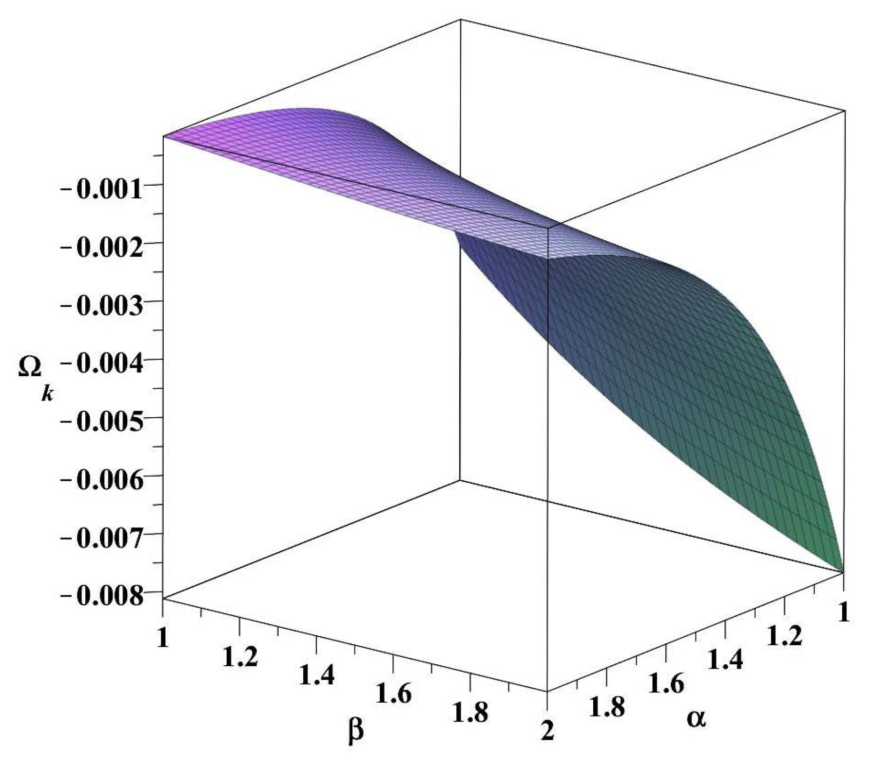
Albeit working on a rather simplified FLRW cosmological model, we envisaged how fractional calculus induced elements (imported to some judicious extent) could change very specific features. Namely, the discussion on a particular application within a FLRW model: it allowed to speculate on the flatness problem of standard cosmology. We are aware of the perhaps uncomplicated assumptions we took in employing therein fractional calculus. Proceeding into more rigorous mathematical computations may require to use far more elaborated expressions, possibly not even those in (23)–(26) but other improved formulae.

Other issues, such as the horizon or structure formation should of course be considered. This surely must and will be discussed in subsequent publications, possibly by other authors whom we challenge to contribute as well. Likewise, other broader cosmologies or matter contents would be important to investigate: more should be done towards appraising fractional quantum cosmology.

6.

A paradigmatic setting in quantum cosmology has been the (harmonic) oscillator, used, within the FRW one-dimensional minisuperspace models, with $H=p_a^2+U\left(a\right)$, $U\left(a\right)\sim a^2$, then $U_{\mathsf{\Lambda }}\left(a\right)\sim a^2-\mathsf{\Lambda }{a}^4$; cf. solutions as DeSitter and conformally coupled scalar field minisuperspace [12].

A rather specific issue, relevant for quantum cosmological applications, would be to have fractional quantum mechanics further explored and elaborated, particularly concerning tunneling within a WKB approach for e.g., potentials of the form $U_{\mathsf{\Lambda }}\left(a\right)\sim a^2-\mathsf{\Lambda }{a}^4$. Being more concrete, exploring the situation (with either $E=0$ or $E\ne 0$) of nucleation from classical forbidden to allowed regions or a transition from classical allowed, through classical forbidden, towards classically allowed domains. Within quantum cosmology, tunneling (nucleation) is usually taken with $E=0$ (as following from the $H=0$ constraint) but a $E_{rad}\ne 0$ has been explored in [29,30] (cf. references therein, too), within concrete applications for the wave function of the universe and (initial) conditions.

Furthermore, since variance can emerge as asymptotic infinite in fractional quantum mechanics [4,6,9,10], then processes could be more likely to occur (or not) regarding Universe nucleation, initial conditions for inflation and its likelihood within standard quantum cosmology versus a fractional framework. This modified setting could be explored with respect to sampling initial conditions.

7.

Finally, simply take and ‘play’, aiming to induce a fractional (quantum gravitational modified) Schrödinger equation, within the principles present in [19]. We could simply directly modify, ad-hoc, the Laplacian therein (in the Schrödinger equation) to further probe it. For instance, about the Bunch–Davies state or a deviation, now within a fractional quantum mechanics setting. Or instead about non-unitarity following from the quantum gravitational corrected Schrödinger equation [19]; could that non-unitarity be re-cast as a consequence either of minisuperspace covariance being lost or, equivalently, fractional time derivative emerging?

It would be thus immensely interesting if a Schrödinger equation bearing gravitational quantum induced corrections [19], but within fractional quantum mechanics, could be investigated, eventually applied to concrete cases. In addition, discussing whether the seeding process from fluctuations in a scalar field $\delta \varphi$ would be ‘easier’ to emerge cf. [9,10]). Or would the Bunch–Davies vacuum, associated with Gaussian states and a Schrödinger equation for matter fields (when dealing with quantum gravitational corrections [12,19,22]) be removed and other quite different state be retrieved (by means of a suitable fractional Schrödinger equation)?

In addition, there is plenty still to be done. Thus, remembering and respectfully borrowing from Leibnitz [1], “(⋯) useful consequences will be drawn”.

References

1. Ross, B. A brief history and exposition of the fundamental theory of fractional calculus. In Fractional Calculus and Its Applications; Lecture Notes in Mathematics; Ross, B., Ed.; Springer: Berlin/Heidelberg, Germany, 1975; Volume 457. [Google Scholar] [CrossRef]
2. Herrmann, R. Fractional Calculus: An Introduction for Physicists; World Scientific: Singapore, 2014. [Google Scholar]
3. Samko, S.G.; Kilbas, A.A.; Marichev, O.I. Fractional Integrals and Derivatives, Theory and Applications; Gordon and Breach: Amsterdam, The Netherlands, 1993. [Google Scholar]
4. Laskin, N. Principles of Fractional Quantum Mechanics. arXiv 2010, arXiv:1009.5533. [Google Scholar]
5. Laskin, N. Fractional Quantum Mechanics; World Scientific: Singapore, 2000. [Google Scholar] [CrossRef] [Green Version]
6. Laskin, N. Fractional quantum mechanics. Phys. Rev. E 2000, 62, 3135–3145. [Google Scholar] [CrossRef] [PubMed] [Green Version]
7. Laskin, N. Fractional Schrödinger equation. Phys. Rev. E 2002, 66, 056108. [Google Scholar] [CrossRef] [PubMed] [Green Version]
8. Laskin, N. Fractional Quantum Mechanics and Levy Path Integrals. Phys. Lett. A 2000, 268, 298–305. [Google Scholar] [CrossRef] [Green Version]
9. Hasanab, M.; Mandal, B. Tunneling time in space fractional quantum mechanics. Phys. Lett. A 2018, 382, 248–252. [Google Scholar] [CrossRef] [Green Version]
10. De Oliveira, E.; Vaz, J. Tunneling in fractional quantum mechanics. J. Phys. A Math. Theor. 2011, 44, 185303. [Google Scholar] [CrossRef]
11. Halliwell, J. Derivation of the Wheeler-DeWitt equation from a path integral for minisuperspace models. Phys. Rev. D 1988, 38, 2468. [Google Scholar] [CrossRef] [PubMed]
12. Kiefer, C. Quantum Gravity, 3rd ed.; Oxford University Press: Oxford, UK, 2012. [Google Scholar]
13. Kleinert, H. Path Integrals in Quantum Mechanics, Statistics and Polymer Physics, and Financial Markets, 3rd ed.; World Scientific: Singapore, 2004. [Google Scholar] [CrossRef] [Green Version]
14. Kyprianou, A.E. An Introduction to the Theory of Lévy Processes, 2nd ed.; Springer: Berlin/Heidelberg, Germany, 2014. [Google Scholar] [CrossRef] [Green Version]
15. Mandelbrot, B. The Pareto-Lévy Law and the Distribution of Income. Int. Econ. Rev. 1960, 1, 79–106. [Google Scholar] [CrossRef] [Green Version]
16. Paul Lévy, P. Calcul des Probabilités; Gauthier-Villars: Paris, France, 1925. [Google Scholar]
17. Pinsker, F.; Bao, Y.Z.W.; Ohadi, W.; Dreismann, A.; Baumberg, J.J. Fractional quantum mechanics in polariton condensates with velocity dependent mass. Phys. Rev. B 2015, 92, 195310. [Google Scholar] [CrossRef] [Green Version]
18. Wu, J.-N.; Huang, C.-H.; Cheng, S.-C.; Hsieh, W.-F. Spontaneous emission from a two-level atom in anisotropic one-band photonic crystals: A fractional calculus approach. Phys. Rev. A 2010, 81, 023827. [Google Scholar] [CrossRef] [Green Version]
19. Kiefer, C.; Singh, T.P. Quantum Gravitational corrections to the functional Schrödinger equation. Phys. Rev. D 1991, 44, 1067. [Google Scholar] [CrossRef] [PubMed]
20. Cresson, J. Fractional embedding of differential operators and Lagrangian systems. J. Math. Phys. 2007, 48, 033504. [Google Scholar] [CrossRef] [Green Version]
21. Inizan, P. Homogeneous fractional embeddings. J. Math. Phys. 2008, 49, 082901. [Google Scholar] [CrossRef] [Green Version]
22. Kiefer, C.; Kwidzinski, N.; Piontek, D. Singularity avoidance in Bianchi I quantum cosmology. Eur. Phys. J. C 2019, 79, 686. [Google Scholar] [CrossRef]
23. Iomin, A. Fractional evolution in quantum mechanics. Chaos Solitons Fractals 2019, 1, 100001. [Google Scholar] [CrossRef]
24. Moniz, P.; Jalalzadeh, S. Challenging Routes in Quantum Cosmology; WSP: Singapore, 2020; Chapter 7. [Google Scholar] [CrossRef]
25. Tipler, F.J. Interpreting the wave function of the universe. Phys. Rep. 1986, 37, 231. [Google Scholar] [CrossRef]
26. Jalalzadeh, S.; Capistrano, A.J.S.; Moniz, P.V. Quantum deformation of quantum cosmology: A framework to discuss the cosmological constant problem. Phys. Dark Universe 2017, 18, 55. [Google Scholar] [CrossRef] [Green Version]
27. Mukhanov, V. Physical Foundations of Cosmology; University Press: Cambridge, UK, 2005. [Google Scholar]
28. Allday, J. Quarks, Leptons and the Big Bang, 2nd ed.; Institute of Physics Publishing: Bristol, UK, 2001. [Google Scholar]
29. Bouhmadi-Lopez, M.; Moniz, P. Quantization of parameters and the string landscape problem. JCAP 2007, 4390705, 005. [Google Scholar] [CrossRef]
30. Brustein, R.; de Alwis, S.P. Landscape of String Theory and The Wave Function of the Universe. Phys. Rev. D 2006, 73, 046009. [Google Scholar] [CrossRef] [Green Version]
Figure 1. The plot of Ω 0 , k = 1 for n = 500000 and | Γ | = 1 .
Mathematics 08 00313 g001