In this section, we present the numerical results based on our novel iterative splitting methods for nonlinear ordinary and partial differential equation. We verified our theoretical results of the error-estimates and applied the shifted iterative splitting methods as a new-solver class.
4.1. First Numerical Example: Bernoulli Equation
In the first example, we apply a nonlinear differential equation, which is given as the Bernoulli equation, see
For the Bernoulli equation, we can derive analytical solutions as reference solutions, see [
15,
22]. The analytical solutions are given as
Using
we find that
, so
For the applications, we apply the following parameters, , , , , , , and .
We apply the following operators for the splitting.
We apply backward Euler method to approximate the derivative in each subinterval
, and solve the resulting equation by using the fixed point method and Newton’s method with tolerance
allowing a maximum of three iterations. The accuracy of the methods is assessed by comparing the numerical result
with the analytical solution
u given by (
37). We compute the maximum and mean difference at the nodes
, according to
and
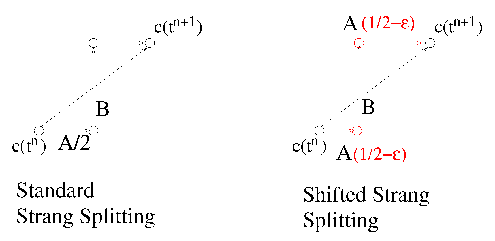
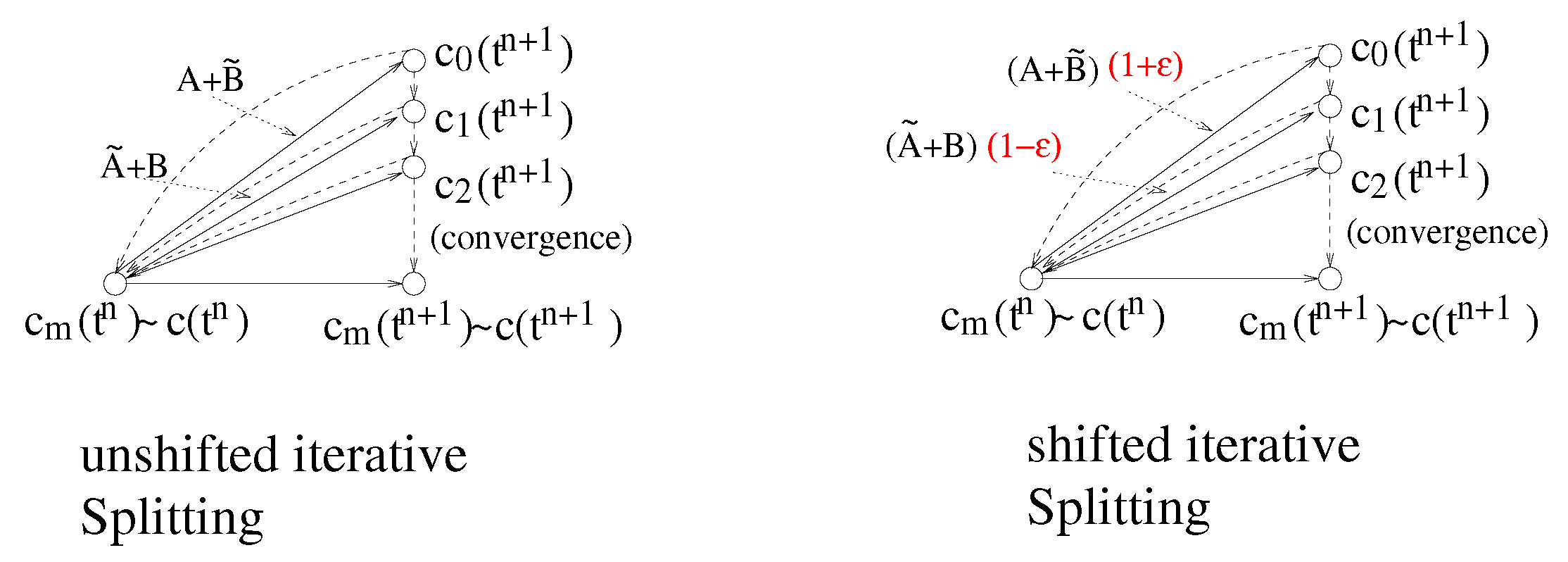
For the Shifted Strang–Marchuk splitting, we analyze the accuracy (with respect to the analytic solution) and the cost of the algorithm for different tolerances and coarsening factors , where we have set . Taking larger values of reduces the number of time intervals, but increases the number of tentative steps, where the must be reduced in order to satisfy the error tolerance criterion. The value of has been experimentally chosen in order to minimize the total number of steps.
In each splitting step, the differential equation is approximated by back-Euler’s method and solved using the fixed point (BEFP) or Newton’s (BEN) methods. The cost of the algorithm and the final accuracy depend on the error tolerance and the coarsening factor . We compare the shifted ABA-operator splitting method with the shifted variants of the iterative splitting methods above considered.
Table 1 shows that the accuracy is roughly proportional to the square root of the tolerance
, and the number of functional evaluations is inversely proportional to the same quantity. Newton’s method requires less iterations to fulfill the tolerance; thus, if the number of time steps is similar to that of the fixed point method, it needs less functional evaluations. Nevertheless, Newton’s method also evaluates the derivative, which reduces its advantage over the fixed point method.
For the Shifted Linear Iterative Splitting method, we take
. We obtain similar accuracies to Strang–Marchuk’s algorithm working now with higher error tolerances
, as it is shown in
Table 2. The accuracy is of the same order as
, whereas the computational cost is slightly higher than the cost of Strang–Marchuk’s algorithm.
The results for the Shifted Quasilinear Iterative Splitting, see
Table 3, are quite alike to the ones of the linear splitting. Increasing the number of iterations,
, results in a linear increment of the cost without any accuracy improvement.
4.2. Second Numerical Example: Mixed Convection–Diffusion and Burgers Equation
In the second numerical example, we apply coupled partial differential equation (PDE). We apply a coupling of a convection–diffusion equation with a Burgers’ equation in 2D, which is called mixed convection–diffusion and Burgers equation (MCDB), and given as
where the domains are given as
and
. The viscosity is
.
For such an mixed PDE, we can derive an analytical solution, which is
where we can derive the right hand side
.
By considering the following operators
The MCDB Equation (
38) is splitted into the Burgers’ term,
A and the convection–diffusion term,
B and we obtain the operators:
We deal with different viscosities: low viscosity
, high viscosity,
. The spatial domain is discretized taking a rectangular mesh with
intervals and applying standard second order divided difference approximations. The resulting differential system is solved by the same methods as in the previous example. The coarsening strategy applied here when
is
where
is the vector norm of the computed values in the nodes
at each time step.
For the shifted Strang–Marchuk splitting method we take and different values of .
Table 4 shows the results of solving the equation with low viscosity
using different tolerances. The solutions of the differential equations are approximated by using back-Euler fixed point method (BEFP) or back-Euler–Newton’s method (BEN). Both methods perform similarly in cost and accuracy in this case.
The corresponding results for solving the equation with high viscosity,
, are shown in
Table 5. BEFP requires much more time steps then BEN, but reaches more accuracy.
For the linear and quasilinear shifted iterative splitting methods we take
and the same coarsening strategy.
Table 6,
Table 7,
Table 8 and
Table 9 show the cost and the accuracy in the low and high viscosity cases for the shifted linear and quasilinear iterative splitting methods using the back-Euler fixed point method and back-Euler Newton’s method as solvers.
The shifted linear and quasilinear iterative splitting methods give similar results in all the considered cases. The behavior of the back-Euler fixed point method is worse in the low viscosity case than in the high viscosity case, as in the shifted Strang–Marchuk splitting method.
4.3. Third Numerical Example: Convection-Diffusion-Reaction Equation
In the third numerical example, we deal with a PDE, which is a convection–diffusion–reaction equation in 3D (CDR), see the example in [
23]:
where we have
,
a diffusion matrix,
is the velocity field,
k is a reaction parameter, and
,
.
We can have a special analytical solution for an instantaneous point source, which is given as:
We have the following parameters.
instantaneous point source: , ,
initial start at , where we initialise the equation with ,
the diffusion parameters are given as all other parameters are 0,
the velocity is given as ,
the reaction parameter is given as .
By considering the following operators, we decouple into the fast velocity–reaction part and the slow diffusion parts:
we split (
50) in fast and slow parts
The equation is spatially discretized taking a number, of equal subintervals in each direction in , and approximating the spatial derivatives by standard second order divided differences, resulting in a linear differential system.
We first check that the discretization error decreases with the size of the spatial subintervals by solving the differential system using Heun’s method and Strang–Marchuk method with different number of spatial subintervals. The numerical results
in the node points
are compared with the analytical solution
in the same points at the final time
, computing the maximum and the mean absolute differences as before.
Table 10 shows that there is no significant difference between both methods.
Now we fix the number of spatial subintervals
and analyze the performance of the adaptive methods for the CDR example. To estimate the convergence of the methods, we compare their results with the approximation obtained by integrating the differential equation by Heun’s method using the same time steps.
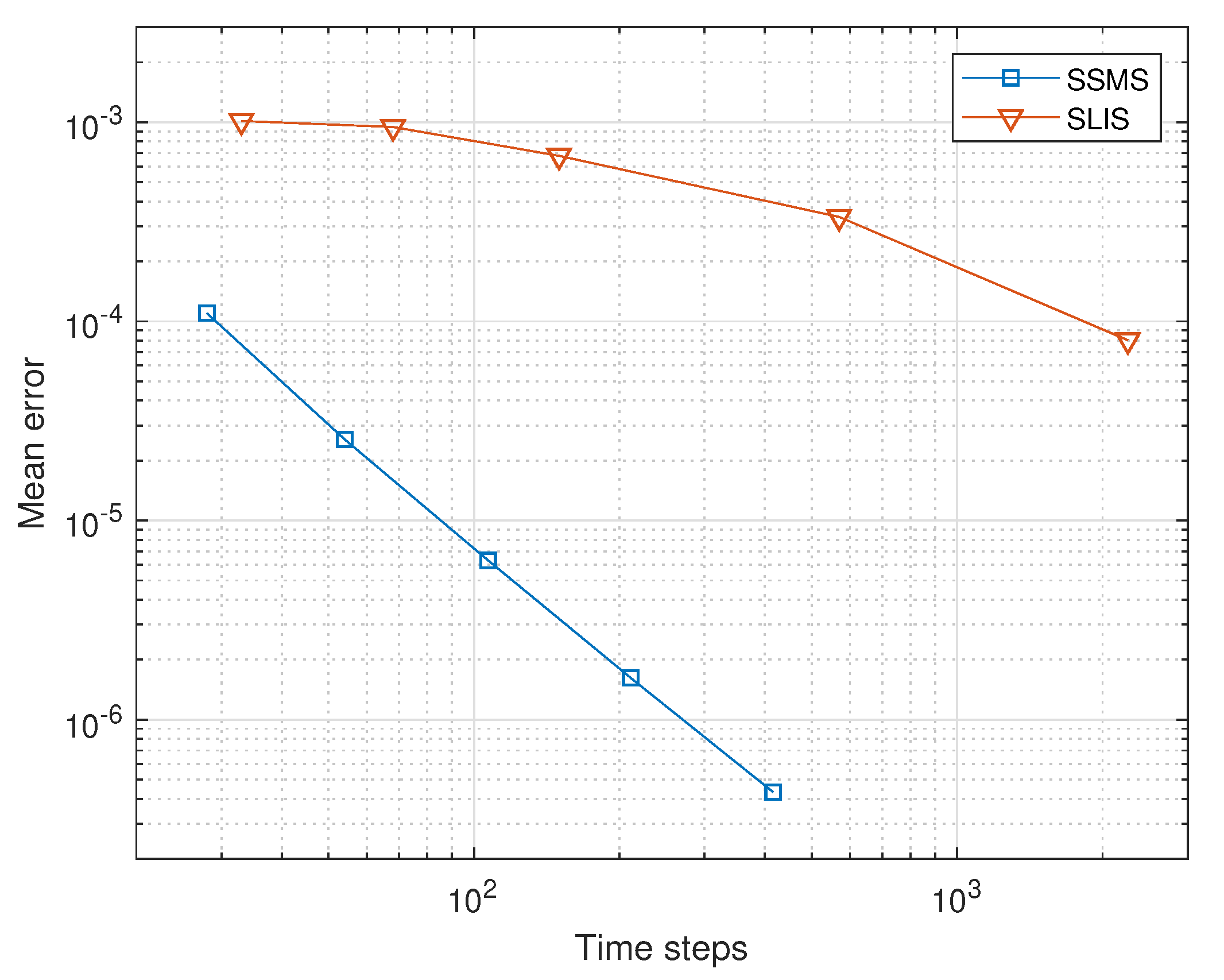
Table 11 shows the results of the shifted Strang–Marchuk splitting and the shifted linear iterative splitting for different tolerances,
. Lower tolerances produce lower maximum and mean errors but require more time steps. The relationship between the number of time steps and the mean error is depicted in
Figure 3.
Remark 4. In the Figure 3, we see the differences in the convergence behaviour between the shifted Strang–Marchuk splitting (SSML) and the shifted linear iterative splitting (SLIS) method. We see in the figure, that the SSML method has only a linear convergence order , the SLIS method has higher order of convergence, here we have at least an order . Therefore the adaptive iterative scheme is much more effective and accurate than the noniterative splitting scheme. The result verified the proposition, that the iterative splitting scheme is a higher order scheme, see [3,15], and that we also conserve the higher order approach in the adaptive version. 4.4. Fourth Numerical Example: Nonlinear Diffusion Equation
Our fourth numerical example is a partial differential equation which is nonlinear diffusion equation in 2D, see the example in [
24].
The multicomponent diffusion equation is based on the idea of a Maxwell–Stefan diffusion equation, which is highly nonlinear, see [
20,
24]:
where we have
a nonlinear diffusion matrix and
,
,
.
An application of such a nonlinear diffusion (NLD) is given by
where we have
and
.
Further, we apply with the following parameters in the NLD Equations (
41) and (
42).
The parameters and the initial and boundary conditions are given as:
Uphill example, which is known as semi-degenerated Duncan and Toor experiment, see [
25]:
and , where we have .
Asymptotic example, which is known as asymptotic Duncan and Toor experiment, see [
25]:
and , where we have .
We apply , where J is the number of spatial grid points.
Based on the explicit discretization method, we have to fulfill the time-step-restriction, which is given as CFL-condition:
.
The computational domains are given with: is the spatial domain and is the time domain.
The initial conditions are as follows.
For the boundary conditions, we apply no-flux type conditions:
We apply the following splitting of the operators with the one-dimensional spatial derivations:
where we have the operators in the following decomposition of the
and
parts with
:
where we have
a symmetric decomposition.
We first check that the non adaptive methods require a very small time step to converge and estimate its convergence by comparing the results doubling successively the number of time steps. The results are shown in
Table 12 for the direct integration and for the unshifted Strang–Marchuk method. The errors are computed measuring the difference between the result obtained with a given number of time steps and the result with twice that number at every shared temporal and spatial node. The error estimates for the Strang–Marchuk splitting in the case of 40,000 time steps are not available because the method diverges with 20,000 time steps.
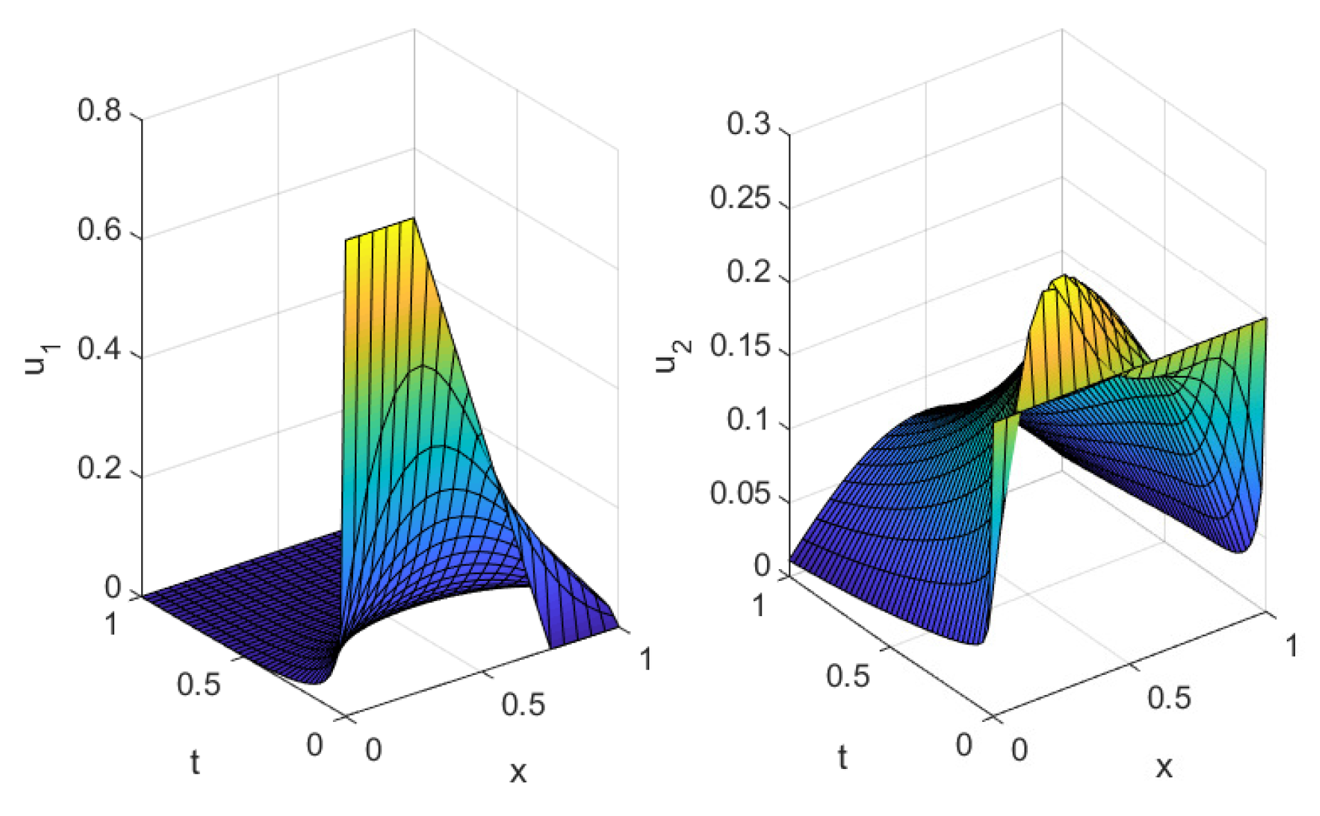
Figure 4 illustrates the uphill phenomenon, where the solutions
and
increase before reaching the stationary state.
The adaptive methods result in an important reduction of the number of time steps obtaining similar error estimations.
Table 13 and
Table 14 show the results for the uphill case and for the asymptotic case of the nonlinear diffusion equation, respectively. Here, the errors are computed by comparing the solution of the shifted methods with the ones obtained by direct integration, using the same time steps as the adaptive method.
The shifted Strang-Marchuk method behaves better for
= 0.03, whereas the shifted linear and quasilinear splitting methods work well for
= 0.03, except for in
Table 15, where the behavior of the considered splitting methods is studied for different splitting weights
.
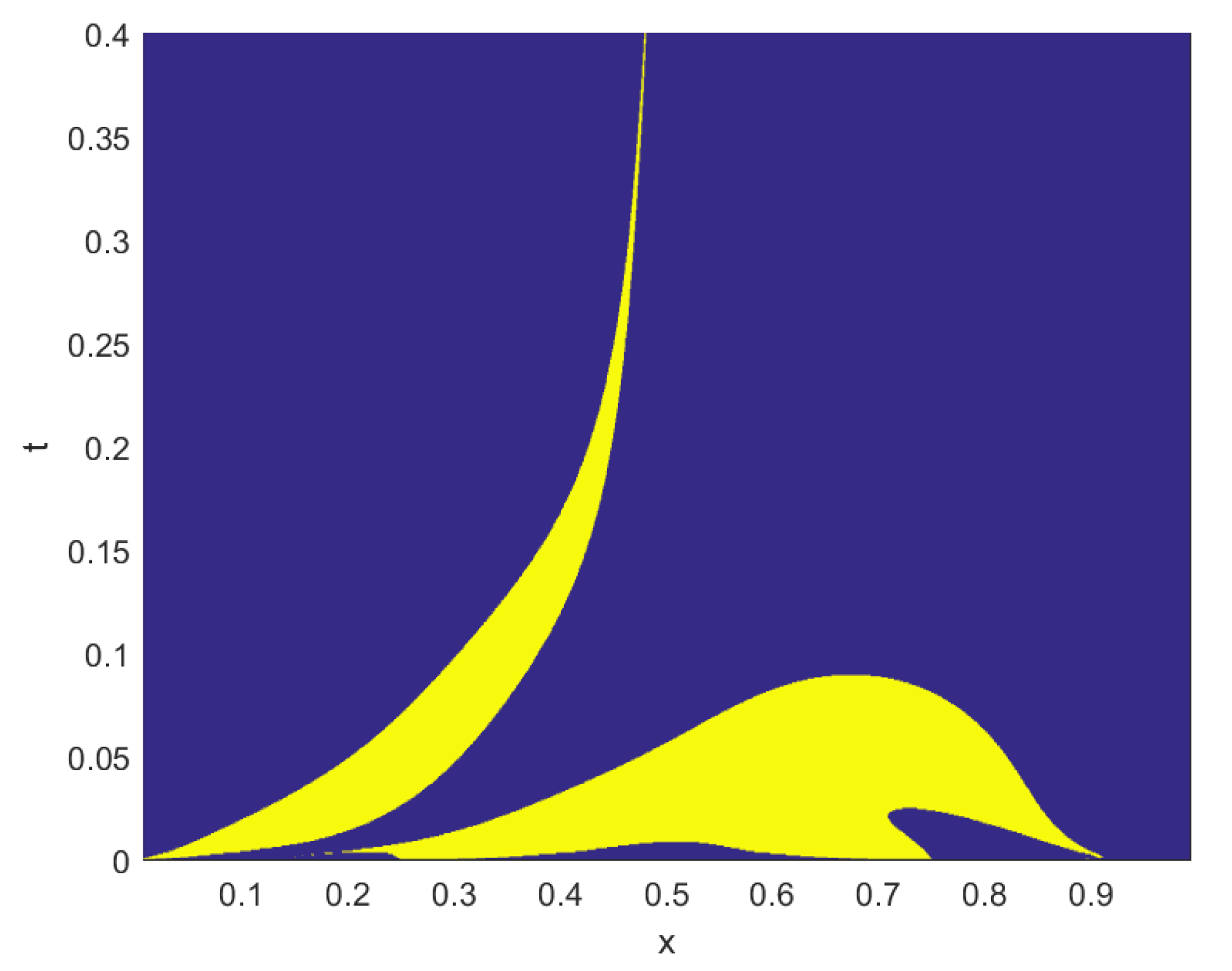
Figure 5 depicts the regions in the space-time plane where the uphill phenomenon takes place, that is where
and
have the same sign. The equation is solved by the shifted linear iterative splitting with
.


