Abstract
In this paper, we discuss iterative and noniterative splitting methods, in theory and application, to solve stochastic Burgers’ equations in an inviscid form. We present the noniterative splitting methods, which are given as Lie–Trotter and Strang-splitting methods, and we then extend them to deterministic–stochastic splitting approaches. We also discuss the iterative splitting methods, which are based on Picard’s iterative schemes in deterministic–stochastic versions. The numerical approaches are discussed with respect to decomping deterministic and stochastic behaviours, and we describe the underlying numerical analysis. We present numerical experiments based on the nonlinearity of Burgers’ equation, and we show the benefits of the iterative splitting approaches as efficient and accurate solver methods.
Keywords:
Burgers’ equation; stochastic differential equation; noniterative splitting; iterative splitting; splitting analysis; deterministic–stochastic splitting MSC:
35K25; 35K20; 74S10; 70G65
1. Introduction
We are motivated to extend noniterative and iterative splitting methods with respect to stochastic Burgers’ equations. We will also present the limits and impacts of our novel schemes; see []. While stochastic Burgers’ equations are important to model nonlinear and stochastic flow problems, they are not straight forward to solve because of their deterministic and stochastic behaviour; see []. Based on the nonlinearity of the flow-term, we add a stochastic reaction term that influences the speed of the underlying deterministic flow. These stochastic Burgers’ equations are nowadays important and are applied (for example) in high-temperature superconductors (see []), growth problems, or especially epitaxial growth []. Stochastic behaviour is important to model oscillations in the flow-problems; see []. Many applications in transport phenomena can be modelled with uncertainties by combining deterministic and stochastic operators; see [].
Our motivation is to explain the benefits of the splitting approaches, which allows to concentrate on each part of the equation; that is, the deterministic/nonlinear part and the stochastic/reaction part; see [,,].
The splitting schemes are considered with respect to the two behaviours of the stochastic Burgers’ equations:
- Nonlinear/deterministic transport; see [,]; and
- Stochastic/reaction; see [,].
Here, we consider an extension of the deterministic Burgers’ equation, which is done with an additional stochastic part of multiplicative noise; see [,].
To see the benefits of the different types of the splitting methods; see [,]. We discuss the most significant types, which are the noniterative and iterative approaches; see [,]. Their convergence and accuracy behaviour is studied for both deterministic and stochastic approaches; see [,].
Here, we can test the benefits and drawbacks of the different splitting types with respect to resolving the important processes of the model. Overall, the splitting approaches are important. We apply specialised solver methods for each equation part (e.g., the deterministic part is solve with fast PDE-solvers), while the stochastic part is solved with fast SDE-solvers; see the different behaviours in their numerical approaches in [,].
We consider the benefits and drawbacks of the noniterative and iterative splitting methods, which use different algorithms to solve the model-problem and their numerical errors; see [,]. In particular, we aim to discuss the benefits (e.g., they are fast to implement and simpler to control) and drawbacks (e.g., their accuracy and the lack of decomposing to different physical structures) of noniterative splitting approaches; see [,]. We will also discuss the alternative iterative splitting approaches, whose accuracy is of a higher order and which are physically more adequate but are more delicate to control and more complex to implement; see [,].
We will apply operator splitting approaches, which are designed to consider decoupable operator equations and solve them with adequate solver methods for each decoupled equation; see [].
Here, we apply the technique to decompose into deterministic and stochastic operators; see [,].
The splitting approaches are defined in two directions:
- Noniterative schemes: Here, we discuss the Lie–Trotter-splitting and Strang-splitting schemes; see [,], which we call AB-, ABA- and BAB-schemes.
- Iterative schemes: Here, we discuss Picard’s iterative schemes; see [].
The deterministic splitting approaches can be extended to decoupable deterministic and stochastic approaches, which are given in the numerical stochastics literature; see, for example, [,,].
The benefit of these splitting approaches is that they decompose different operators, which can be discussed and solved numerically with more optimal methods.
In the case of the underlying stochastic Burgers’ equation, we apply the following decomposition:
- Deterministic part: We solve the deterministic part with fast conservation methods; see [,].
- Stochastic part: We solve the stochastic part with fast solutions for thee stochastic ordinary differential equation; see [,].
The rest of this paper is structured as follows: The model is given in Section 2. The numerical methods are discussed in Section 3. The numerical analysis is presented in Section 4. In Section 5, we present the numerical simulations. Finally, we draw our conclusions and summarise our results in Section 6.
2. Mathematical Model
In our model, we concentrate on nonlinear stochastic PDEs (SPDEs). These are related to nonlinear PDEs in fluid-dynamics models, where random phenomena play an important role; see, for example, []. We concentrate on Burgers’ equations, which combine nonlinear advection and diffusion, and are often used as test equations for Navier-Stokes equations; see []. In the following, we concentrate on a stochastic Burgers equation (SBE) that is driven by deterministic or stochastic reaction terms, while the stochastic reaction terms are given as linear multiplicative noise; see [,].
The nonlinear SPDE in the notation of a stochastic Burgers’ equation (SBE) is given as:
where c is the velocity-field and the solution of the stochastics Burgers’ equation. is a positive diffusion coefficient, is a two-sided one-dimensional Wiener process. is the nonlinear flux-function, such as . Furthermore, f is globally Lipschitz continuous in . is a nonlinear function, which measure the deterministic reaction part. Meanwhile, is multiplicative noise function and Lipschitz continuous in c, which measures the amplitude of the noise of the stochastic reaction part. is an initial condition. Finally, is the end-time of the time-domain and is the right-hand boundary of the space-domain.
If we consider each part of the full model separately, then we have to deal with the following two models:
- Burgers’ equation (deterministic part)which is a simplified model for turbulence; see []. The Burgers’ Equation (6) consists of two different modelling parts, which are given as follows:
- -
- Nonlinear advection part (), which represents the nonlinear advected velocity of the fluid, and
- -
- Linear diffusion part (), which represents the thermal fluctuations of the fluid.
- Reaction equation (stochastic part)which is a simplified model for stochastic dynamical system (e.g., a reactive specie); see [], and consists of two parts:
- -
- Deterministic part, which represents the reaction of the species, and
- -
- Stochastic part, which represents the fluctuations of the reactive species.
The modelling equations, which are based on deterministic and stochastic reactions terms (especially multiplicative noise for the stochastic part), are used to model complicated turbulences and non-equilibrium phase transitions; see [,]. These models are also used to deal with randomly fluctuating environments [] and disturbances that are modeled with parameters based on uncertainties; see []. For our application, the disturbances and noises are modelled as one-dimensional white noise in Burgers’ equation under the framework of SPDE, see []. For higher-dimensional white noise, many modelling problems are widely considered in engineering and physical research for complex systems; for example, group consensus of multi-agent systems; see []. These applications are directed in networks with noise and time delays; see [].
In the following, we study the stochastic Burgers’ equation (SBE) with a nonlinear advection part and a stochastic reaction part. The SBE can be formulated as a stochastic conservation law, which is driven by Gaussian noise; see []. In the following, we call this formulation of the SPDE a stochastic balance equation; see [,], while we deal with the following SBE:
where is the multiplicative noise function, is the nonlinear flux function and is a Wiener process.
Here, we can see two effects, which are often conflicted: while the nonlinearity of the SBE would steepen the fronts into discontinuous shocks, the stochastic part of the SBE is more of a diffusion process and it smooths fronts away. We have the motivation to see how solver methods could extract and balance these two effects.
3. Numerical Methods
In this section we will describe the different solver methods and we will discuss them in detail. For the numerical methods, we consider splitting approaches, which decompose the two parts of the SBE (i.e., the deterministic pure Burgers’ operator and the stochastic reaction equation). Based on the stochastic balance Equation (6), we apply the following notation for the stochastic Burgers’ equation in a viscid form:
where is random white noise; see [].
Here, we deal with two splitting ideas:
- Noniterative splitting approach, which is given as:
- -
- AB-splitting: in the first step we apply operator A and in the second step we apply operator B; see for the stochastic SDEs []. This is also known as Lie–Trotter scheme; see [].
- -
- ABA splitting: in the first step we apply operator A with a half timestep, in the second step we apply operator B with a full time step and in the third step we again apply operator A with a half time step; for the SDEs; see []. This is also known as Strang-splitting scheme in the deterministic version for the ABA-version; see [],
- -
- BAB splitting: in the first step we apply operator B with a half timestep, in the second step we apply operator A with a full time step and in the third step we again apply operator B with a half time step; see for the SDEs []. This is also known as Strang-splitting scheme in the deterministic version for the BAB-version; see [].
We directly split the full Equation (9) into the parts:
- -
- The deterministic part:where we have the solution
- -
- The stochastic part:where we have the solution
- Iterative splitting approach, which is given as:
- -
- Picard’s fixpoint scheme; see [,], this splitting approach is based on fixpoint-iterations; see [], which are used to approximate ordinary or semi-discretised partial differential equations. The convergence theory is based on the local version of the theorem of Picard-Lindelöf; see []. These iterative schemes can be extended to stochastic partial differential equations. They are also effective and robust in the implementation; see [,].
- -
- Iterative operator splitting; see [], here we use an extension of the Picard’s fixpoint scheme; see []. The idea is to switch between the different operators of the differential equation. In other words, we deal with the different operators, which are directly solved in the iterative process, and the other parts of the operators, which are frozen with previous iterative solutions and used as on the right-hand side, see [,]. The convergence theory is similar to Picard’s fixpoint scheme but it generalises the results for multiple operators; see [,].
- -
- Waveform-Relaxation scheme; see [], this splitting approach is a continuous-time iterative method; see [,]. We have a given function, which approximates the solution and calculates a new approximation along the whole time-interval of interest. Meanwhile, the iterates are functions in time, which we them waveforms. They are often discussed with respect to the Jacobian- and Gauss-Seidel waveform relaxation schemes, which differs based on the diagonal new iterates. In other words, we have the Jacobian-form or the diagonal and lower diagonal new iterates, and also the Gauss-Seidel-form; see [].
- In the following, we concentrate on Picard’s fixpoint scheme, which applies a successive approximation to the nonlinear and stochastic terms; see [].
- We iteratively solve the full Equation (9) with respect to:where i is the iteration index ( and is the starting solution, such as . We have the stopping criterion of the iterative scheme with or , while is an error bound, such as .
- Then, we indirectly solve the deterministic parts. We then couple the solution with a convolution with the stochastic part and apply the iterative steps; see []:
- -
- Solution of the deterministic part:where we assume to deal with a well-posed deterministic Burgers’ equation and can apply a general Cole-Hopf transformation method; see [,]. Then, the analytical solution exists and we can apply it as:
- -
- Convolution with the stochastic part:where we have the solution
Based on separating the deterministic and stochastic operators of the full model, we assume that we can apply the following numerical approaches, which are highly accurate and fast solver methods; see also [,]:
- Deterministic solver for the pure Burgers’ equation: This is a finite volume discretisation for the space with the conservation law solver of Engquist-Osher; see [,].
- Stochastic solver for the stochastic differential equations (SDEs): This is either a Euler-Maruyama solver, a Milstein solver or a stochastic RK solver; see [,].
Remark 1.
We applied the following noniterative splitting approaches (i.e., the -, - and -splitting approaches) and iterative splitting approaches (i.e., the iterative schemes with ). In Section 3.1, we present the noniterative splitting approaches. In Section 3.2, we present the iterative splitting approaches, which are studied and later applied to the numerical experiments.
3.1. Noniterative Splitting Approaches
A main benefit of the noniterative splitting approaches is that they offer a direct (noniterative) solution in one-step, which avoids the need for additional solver steps; see []. Therefore, they are simple to implement and fast in computation, see []. However, one of their drawbacks is that it is difficult to obtain higher order methods; see []. Therefore, we have to apply solvers for nonlinearities that are more delicate; see []. Therefore, we consider the ideas that are given by the exponential splitting methods, such as Lie–Trotter schemes; see [,]. Here, we compute the numerical results for each operator-equation; see Equations (17)–(19), and we couple the results as an initial value of the successor operator-equatio; for example, we apply the results of Equation (17) as an initial value for the Equation (19); see also [].
- AB splitting:
- We use the following AB splitting approaches:
- (a)
- We initialise with and go on for steps :
- (b)
- A-part: We solve equation part Awith time-step and we obtain the solution
- (c)
- B-part: We solve equation part Bwith time-step and we obtain the solutionwhere we obtain .
- (d)
- If we have , then we are done and we obtain the solutions, otherwise we do goto Step (a).
- ABA splitting:
- We use the following ABA splitting approaches:
- (a)
- We initialise with and go on for steps :
- (b)
- A-part: We solve equation part Awith time-step and we obtain the solution
- (c)
- B-part: We solve equation part Bwith time-step and we obtain the solution
- (d)
- A-part: We solve equation part Awith time-step and we obtain the solution .
- (e)
- If we have , then we are done and obtain the solutions, otherwise we do goto Step (a).
- BAB splitting:
- We use the following BAB splitting approach:
- (a)
- We initialise with and go on for steps :
- (b)
- B-part (): We solve equation part Bwith time-step and we obtain the solution
- (c)
- A-part (): We solve equation part Awith time-step and we obtain the solution
- (d)
- B-part (): We solve equation part Bwith time-step and we obtain the solutionwhere we obtain .
- (e)
- If we have , then we are done and obtain the solutions, else we do goto Step (a).
3.2. Iterative Splitting
The benefits of the iterative splitting schemes are their relaxation behaviour and the possibility to gain higher order results for each iterative cycle; see []. The underlying idea is a successive relaxation scheme, which we obtain based on a fixpoint scheme higher accuracy. This means that we apply the solver method several times in the same time-intervals and we improve the solutions iteratively; see []. Therefore, it is important to have very fast underlying solver-schemes, if possible analytical schemes, such that we could save computational time and optimise the number of iterative cycles.
To apply the iterative approaches, we can apply the iterative solvers before or after a spatial discretisation, as follows:
- Iterative splitting after the discretisation, we apply iterative schemes for the nonlinearities.
- Iterative splitting before the discretisation, we apply the iterative scheme to decompose the differential equation into a kernel and perturbation term.
Remark 2.
Based on the way of applying the iterative scheme, we see that if we apply the iterative scheme before the discretisation, then we can obtain higher order results based on improving the numerical integration of the time-variables. Therefore, the iterative steps allow us to obtain more accurate results, as for the standard AB-, ABA- and BAB-splitting methods.
3.2.1. Iterative Scheme after Discretisation
We have the following SDE in continuous form and we apply the sequences with time-step as:
and in the SDE form we apply the sequences with time-step as:
We apply the discretisation in time (Milstein-scheme) and space (finite-volume scheme), and we obtain:
where we have the initialisation .
The solution of the Burgers’ equation is given as:
while we apply for the linearisation in the Burgers’ equation.
We apply a fixpoint-scheme to improve the standard Milstein scheme (41) and we obtain the iterative scheme as:
where we have the iterative cycles with with the starting condition with and the stopping criterion with or , where is an error-bound, such as .
We then apply the solution of the Burgers’ Equation (42) and obtain the improved iterative scheme as:
where we have the initialisation .
We deal with the following iterative splitting approaches:
- Standard Milstein-scheme of second order ():which is a first order approach and similar to the AB-splitting approach.
- Second order iterative splitting approach (related to the standard Milstein-scheme of second order) ():where and obeys the Gaussian distribution with and .Here, we obtain a second order approach, which is similar to the ABA- or BAB-splitting approach.
Remark 3.
If we apply the iterative scheme after the discretisation in time, then we have similar behaviour as for the noniterative splitting approaches. Here, we could gain at least the results of the ABA- or BAB-splitting approaches. A more improved iterative splitting approach can be obtained: if we apply the iterative scheme before the discretisation in time, then we could apply higher order numerical integration methods and gain based on the iterative approaches higher order results above the ABA- or BAB-splitting approaches.
3.2.2. Iterative Scheme before the Dicretisation
We have the following iterative splitting approaches before the discretisation:
We have with:
where we have the initialisation .
We have the solution
with initialisation and .
We deal with the following iterative splitting approaches: First order iterative splitting approach (related to the AB-splitting approach, which means with the rectangle rule and the semi-analytical approach):
- (Initialisation):where .
- (first step):where we apply the Ito’s rule with a first order scheme (Euler-Maryama-scheme) and obtain:where and obeys the Gaussian distribution with and .
We improve the order to 2 with the Milstein approach in the stochastic term and obtain:
(while is linear and not dependent of c, we only have to apply the derivative to ).
The algorithm for is given in Algorithm 1. We have to compute the solutions for .
| Algorithm 1.We start with the initialisation(initial value) and. |
|
Second and third order iterative splitting approach (related to the ABA-splitting approach, which means with the rectangle rule and the semi-analytical approach):
The next algorithm for is given in Algorithm 2, we improve the last with an underlying ABA-method. We have to compute the solutions for .
| Algorithm 2.We start with the initialisation(initial value) and. |
|
The next algorithm for is given in Algorithm 3, we improve the last with additional intermediate time-steps, which are computed by an underlying ABA-method. We have to compute the solutions for .
| Algorithm 3.We start with the initialisation(initial value) and. |
|
In Figure 1, we present the different starting conditions based on full- or half-time steps for the iterative splitting approaches, which are applied in Algorithms 2 and 3.
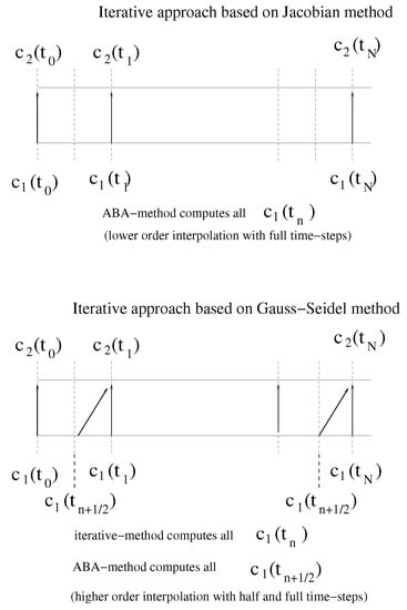
Figure 1.
Function and visualisation of the iterative splitting approach for : In the upper figure, we apply an iterative splitting approach based on the Jacobian-method. Here, we apply for the initialisation of the -values for the full time-steps an ABA-method. Therefore, we obtain a lower order interpolation for the itertative approaches of the -values. In the lower figure, we apply an iterative splitting approach based on the Gauss-Seidel-method. Here, we apply for the initialisation of the -values for the full time-steps an iterative method and additional for the half step an ABA-method. Therefore, we obtain a higher order interpolation for the iterative approaches of the -values. We improve the starting conditions for the iterative splitting approach with and obtain higher order approaches.
Remark 4.
We also improved the starting condition based on the midpoint-rule, such that we obtain a second order approach for the starting solutions of the iterative approach. While we could apply additional iterative splitting steps, we could gain more than second order approach if we improve the numerical integration parts (e.g., Simpson-rule; see []) and also the stochastic integration parts (e.g., higher stochastic schemes; see [,]). In Appendix A.1, we present more details about the derivation and improvments of the underlying splitting approaches.
In Figure 2, we present the important ideas of improving the iterative splitting method with starting solutions, which are obtained by the AB-splitting method and the ABA-splitting method. While the first order approaches are sufficient, the AB-splitting method and the second order approaches are done with the ABA-splitting method. Therefore, the starting conditions of the iterative splitting approach are of first or second order, such that we could improve the iterative splitting approach with additional steps to higher approaches than of the second order; see also [].
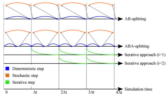
Figure 2.
Illustration of how the iterative algorithms work in principle. The idea is a boot-strap algorithm, which improves the starting conditions of the iterative splitting approach. In the upper figure, we present the AB-splitting method. The first step is deterministic and the second step is stochastic. In middle figure, we present the ABA-splitting method. The first step is deterministic, the second step is stochastic step and the third step is deterministic, and we obtain a second order approach. In the lower figure, we have the iterative splitting approach of , which uses a second order starting condition of the ABA-splitting method and improves the results with an iterative step to higher order results. These results of the iterative splitting approach of are used as a starting condition for the iterative splitting approach of , we also could improve the results with more accuracy and so on; see also [].
4. Numerical Analysis
In the following, we discuss the iterative splitting approach, which is given in Algorithms 2 and 3.
The outline of the analysis is given with respect to a fixpoint scheme, where we analyse the convergence and the convergence rates to the fixpoint-solution; see also [,]. In the numerical analysis, we concentrate on the new iterative algorithms and we present the approximation to the fixpoint of the solutions.
The relaxation scheme is given with the iterative splitting scheme as:
where we have with the start condition .
We apply the integration and have the solution
with initialisation and .
Definition 1.
We have and . Furthermore, G is Lipschitz continuous on Ω with Lipschitz-constant γ if
for all .
We have the following assumptions:
Assumption 1.
We have the Lipschitz-continuous functions , which is a function of the pure deterministic Burgers’ equation, and , which is a function of the pure stochastic reaction equation, while we also assume that is Lipschitz continuous.
Then, we have the following Lemma:
Lemma 1.
We have and . Furthermore, and are contraction mappings on Ω and boundable. Then, we obtain, that and are Lipschitz continuous with constants and .
Proof.
We have
While the operator for the pure deterministic Burgers’ equation is bounded with respect to and we obtain for sufficient small and .
Furthermore, we have
while the operator is bounded and Lipschitz continuous. □
In the following Theorem 1, we present the convergence rate of the iterative splitting scheme (60), which allows us to obtain higher order results based on the number of the iterative-steps. Therefore, we are much more flexible to achieve higher accurate results as for the noniterative methods, while we have an additional freedom-degree.
Theorem 1.
We assume, that Ω is a closed subset of , and that and are contraction mappings on Ω with Lipschitz-constants and . Then, the iterative scheme (60) converges linearly to with the factor . Furthermore, the convergence rate is given with , where is the uniform time-step and i is the number of iterative steps.
Proof.
We apply the iterative scheme:
and evaluate the integral based on the Taylor-Ito scheme at the integration point and obtain the accuracy of the Milstein-scheme, which is given as follows:
- Step 1: Convergence to fixpoint , which is the solution of the iterative scheme:
We apply the difference of the and iterative solution, and obtain:
where we assume the constants and are bounded and with sufficient small and .
We apply the recursion and obtain:
where we obtain .
Then, we obtain for .
- Step 2: Convergence-rate with respect to the iterative cycles:
We apply the difference of the fixpoint-solution and and apply the result of the first step:
where we have the following estimations:
Furthermore, we have the constants , and with sufficient small and .
We apply the recursion and obtain:
where and , where we assume .
Then, we obtain . □
Remark 5.
We obtain a convergence to the fixpoint of the equation based on the iterative scheme. We also obtain an acceleration of the solver-process and a reduction of the numerical error with additional iterative steps. Furthermore, we obtain an accuracy of , which is the half accuracy of a deterministic iterative scheme; see []. Here, we also have to improve the numerical integration with respect to higher order schemes, see also more details in Appendix A.2.
Error Measurements
To verify the theoretical results for the iterative splitting scheme in Section 3, we deal with the following numerical error measurements to analyse the different numerical errors in the schemes, see also more details in Appendix A.3. Here, we concentrate on the weak errors; see [].
We present the convergence rates of the following weak errors:
- Weak error with the deterministic Burgers’ equation as a reference solution:where N are the number of solutions of the stochastic Burgers’ equation.
Furthermore, is the solution of the pure Burgers’ equation and is the j-th solution of the stochastic Burgers’ equation. We assume that we have runs of the stochastic Burgers’ equation.
- Weak error with the stochastic Burgers’ equation as a reference solution:where N are the number of solutions of the stochastic Burgers’ equation.
Furthermore, is a j-th reference solution of the stochastic Burgers’ equation, e.g., with a higher order iterative splitting approach and is the j-th solution of the stochastic Burgers’ equation. We assume that we have runs of the stochastic Burgers’ equation.
- Variance for the solution at and -sample paths:we deal with number of seeds and , is the result of the method at in the seed j. Furthermore, we apply for the iterative scheme steps.
Remark 6.
In the numerical examples, we obtain the weak convergence rates with the weak error. Here, we also apply the weak error to obtain an overview to the accuracy of the numerical schemes.
5. Numerical Experiments
The stochastic Burgers’ equation has different application in the real-world problems, such as in the film-deposition or growth-processes; see [,]. In the following numerical experiments, we concentrate on the one-dimensional Burgers’ equation, which is discussed in Section 1; here we assume that the growth process can be simulated in one-direction; see []. Further application of the one-dimensional Burgers’ equation can be applied in the so-called stochastic lubrication problems; see [], which can be reduced to lower-dimensional problems, such as one-dimensional problems; see [].
We first deal with the pure stochastic Burgers’ equation, which is given in Equation (6) and with Dirichlet boundary conditions, which are included in the equation:
where we have the nonlinear function , the space-domain is given with the right-hand boundary with the spatial step-size and the final time point is . The time-step is computed with respect of the CFL-condition; see the Equations (78)–(80), which can be used for each single part or for both terms. We apply a Finite Volumes discretisation for the spatial parts of the Burgers’ equation; see [].
Furthermore, we deal with the CFL condition of the two explicit discretised terms as:
where we use estimates for and where is Gaussian distributed.
Our numerical splitting methods, which are presented in Section 3, are given as:
- AB-splitting,
- ABA-splitting,
- BAB-splitting,
- Iter-splitting (where we apply iterative steps).
In the first run, we present the -errors of the numerical schemes given in Figure 3.
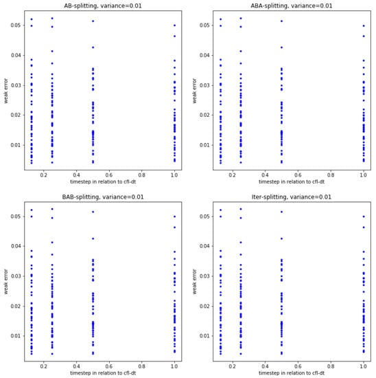
Figure 3.
For the experiments, we have applied the -error given in Equation (73). For the variance of the stochastic process, we used . We applied 10–00 runs for the error evaluation. In the left-hand upper panel, we present the -errors of the AB-spitting approach with different time-steps. We obtain smaller errors for more runs. In the right-hand upper panel, we present the -errors of the ABA-spitting approach with different time-steps. We obtain smaller errors for more runs. In the left-hand lower panel, we present the -errors of the BAB-spitting approach with different time-steps. We obtain smaller errors for more runs. In the right-hand lower panel, we present the -errors of the iterative-spitting approach with different time-steps. We obtain smaller errors for more runs and improved the accuracy.
A comparison of the schemes with the iterative splitting approach is given in Figure 4.
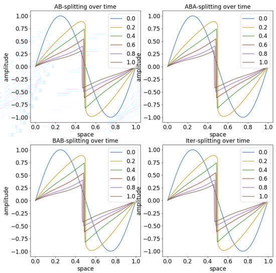
Figure 4.
For the experiments, we have applied the variance and the initial condition . We apply different time-steps, means we start with , which is the -line and the highest number of time-step with , which is the -line. Therefore, we see the influence of the stochastic reaction term, which deformed the initial-solutions. In the left-hand upper panel, we present the solutions of the AB-spitting approach with the different time-steps. In the right-hand upper panel, we present the solutions of the ABA-spitting approach with the different time-steps. In the left-hand lower panel, we present the solutionss of the BAB-spitting approach with the different time-steps. In the right-hand lower panel, we present the solutions of the iterative-spitting approach with the different time-steps.
The errors are defined as errors to compare to the weak and strong convergence, while is defined to see the error of the averaged stochastic solution to the deterministic solution. The idea of looking at errors has been used and discussed in the work []. The detailed errors analysis of the schemes are presented in Figure 5.
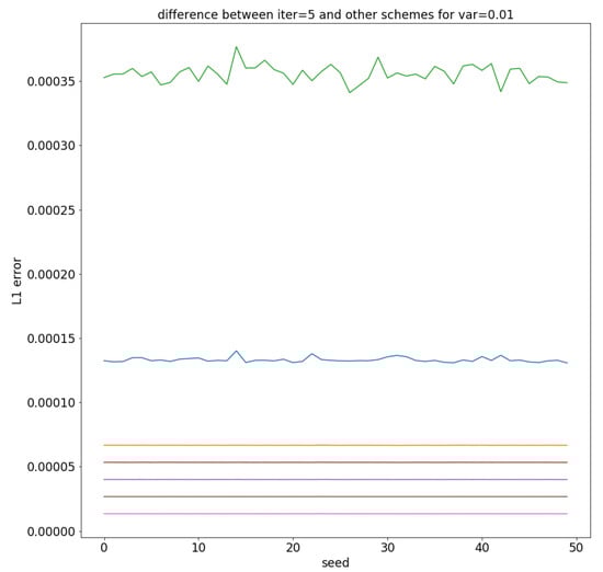
Figure 5.
For the experiments, we have applied the -error given in Equation (74) and apply the iterative splitting approach with as reference solution. For the variance of the stochastic process, we used . In the figure, we have the highest error for the AB-splitting approach, then the ABA-splitting approach and the lowest errors are given with the iterative splitting approach with .
Furthermore, we find that different seeds for the random numbers are more accurate with the stochastic part. We also find problems of the noniterative splitting approaches, which are based on non-relaxational behaviour. For the experiments and the numerical tests, we initialise the pseudo random generator for each new perturbation with a new seed.
The numerical errors between the perturbed and unperturbed solution and the averaged results are given in Figure 6.
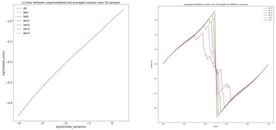
Figure 6.
In the left-hand panel, we see error between unperturbed solution and average over 50 perturbed solutions, while we have applied the -error given in Equation (73). We obtain a relation between small variances and small numerical errors. Therefore the control of higher variances are important. The right-hand panel presents the averaged results for difference variances in the iterative splitting approach method, which are given for the stochastic process with . For high variances around , we obtain a strong influence to the numerical approach.
Remark 7.
For the iterative splitting schemes, we are more flexible and gain higher order results. We can also improve the accuracy of the solutions and see the relaxation with each iterative step. The important part is to accelerate the iterative methods with fast solver parts for the deterministic and stochastic operator. For the model, we saw the reaction behaviour of the oscillating function, which was given with the stochastic part.
In the Remark 8, we discuss the limitation and the impact of the presented splitting methods.
Remark 8.
- Noniterative splitting methods (AB-, ABA-, BAB-splitting):
- -
- Impacts:
- 1.
- Fast implementation of the schemes; see [].
- 2.
- The results are computed in one-step and can be done fast; see [] and [].
- -
- Limitations:
- 1.
- We only achieve second order approaches; see the limits of exponential splitting methods; see [,]. Higher order approaches are delicate to implement (e.g., complex parameters); see [].
- 2.
- Physical structure of the modelling equation is decoupled, while we split in an A-part equation and B-part equation. Consequently, this is physically delicate; see [],
- Iterative splitting methods (Picard’s approximation with :
- -
- Impacts:
- 1.
- Higher order approaches are possible with more iterative steps; see [,,].
- 2.
- The physical structure of the modelling equation is not decoupled, so all the structures are preserved; see [].
- 3.
- The methods are often more stable, while we do not decompose the preserving-structures; see [].
- -
- Limitations:
- 1.
- The implementation of the schemes are more delicate; see [,].
- 2.
- We achieve the solutions in multiple steps, such as (4-steps).
- 3.
- We have to apply fast integration-methods for convolution integrals; see [].
In the concluding section, we give an overview of the results and we outline our next steps.
6. Conclusions
We presented new iterative methods based on Picard’s approximation. These methods are more flexible than the noniterative methods. They also allow us to obtain more accurate results, while we could reduce the error with the iterative steps. We presented the first numerical results with the stochastic Burgers’ equation and multiplicative noise. We saw the stochastic behaviour in the reaction part, which influences the flow of the pure Burgers’ equation. In the future, we aim to apply more delicate SPDEs with respect to mixed time and spatial noises. Here, we apply analytical solutions of parts of the SPDEs (e.g., the Burgers’ equation or the Diffusion equation), and additional fast solutions of the stochastic parts of the SPDEs (e.g., multiplicative conserved noise term depending on x and t). Based on the iterative and noniterative splitting approaches, we define fast-computational interfaces for coupling the deterministic and stochastic equation parts.
Author Contributions
The theory, the formal analysis and the methodology presented in this paper was developed by J.G. The software development and the numerical validation of the methods was done by J.G. The paper was written and was corrected and edited by J.G. The writing–review was done by J.G. The supervision and project administration was done by J.G. All authors have read and agreed to the published version of the manuscript.
Funding
This research was funded by German Academic Exchange Service grant number 91588469.
Acknowledgments
The authors would like to thank Erlend Briseid Storrosten (University of Oslo, Norwey) for the use of his Python-code. Furthermore, the author would like to thank Karsten Bartecki (former student-worker of the author at the Ruhr-University of Bochum, Germany) for his help in the software development and in the numerical experiments, and also for his fruitful discussions. We acknowledge support by the DFG Open Access Publication Funds of the Ruhr-Universität of Bochum, Germany.
Conflicts of Interest
The authors declare no conflict of interest.
Appendix A
In this Appendix, we add more details to the derivation of the used iterative and noniterative schemes, and their applications.
This appendix is divided into the following sections:
- Derivation of the used noniterative and iterative methods; see Appendix A.1.
- Improvements of the integration methods; see Appendix A.2.
- Weak and Strong-Errors; see Appendix A.3.
Appendix A.1. Derivations of the Methods
The SDE is given as:
is a spatial dependent amplitude that changes over time. is a Wiener process (Standard Brownian motion, summation of white noise) over time, and is its time derivative; so, basically white noise. is the diffusion coefficient and can further be time variant or dependent on past values of u. For the sake of brevity, some variables stay omitted.
Ignoring the stochastic part on the right, one can transform the deterministic part and match it against the standard Burgers’ equation (missing diffusion term in this case),
which is solved on a discrete time grid by the conservation law solver with Engquist-Osher in the function (solve conservation law).
A stochastic equation of the form
with real constants and is known as a geometric Brownian motion, which has an exact solution, which is log-normally distributed.
We apply a numerical solution, while we later apply vectorial equations, which can also be coupled by nonlinear functions. Therefore, the simple scalar Equation (A3) is solved by the Milstein method and has the numerical solution:
with drift and diffusion .
Then, via pattern matching to the vectorial form based on the spatial dependencies of the Burgers’ equation, we can deduce a numerical solution for the stochastic part:
Note that the notation of an index like may refer to a derivative in continuous time or time stamp in discrete time. This solver is implemented in the function (solve stochastic differential equation).
- 1.
- AB-splitting
The AB-splitting approach divides the time scale into N intervals. The AB-splitting takes an initial condition and solves the deterministic problem to obtain a solution . The deterministic result is used as an initial condition for the stochastic solver at time t to calculate the final result . This process is repeated N times to obtain the final result.
- 2.
- ABA-splitting
This algorithm works almost identically to the upper one but with a slight modification with regards to the order and length of the solvers. The deterministic solver is used on the first half of a time step, resulting in a helper solution . The stochastic solver than proceeds to calculate a solution on the whole time step and yields another solution , which is used as an initial condition for the deterministic solver to yield the final result for the second half step.
- 3.
- BAB-splitting
As above, but stochastic and deterministic solver are exchanged.
- 4.
- Iterative splitting (after discretisation)
The iterative scheme, here we apply the iterative steps of a stochastic equation of the form
while we obtain an analytical solution of , which is .
We apply the Milstein-scheme plus a fixpoint iterative scheme, which is given as
with drift and diffusion .
- 5.
- Iterative splitting (before discretisation)
Iterative Steps :
Appendix A.2. Improvements to the Integration of the Variation of Constants
(trapezoidal rule):
:
with .
Remark A1.
For higher order integration methods for the variation of constants, we can also apply so-called exponential integrators; see []. These schemes allow us to improve the accuracy with respect to a combination with Runge-Kutta schemes.
Appendix A.3. Numerical Errors: Weak and Strong Error
For the discussion of the numerical errors, we also applied the different numerical errors, which are based on strong and weak errors; see [].
- Strong error:where s is the index of the different seeds, meaning (different Wiener-processes) and is the number of the temporal and spatial steps. Furthermore, is the deterministic reference solution and we test the schemes .
- Weak error:where we assume . Furthermore, s is the index of the different seeds for (different Wiener-processes) and are the number of seeds. is the number of the temporal and spatial steps. Additionally, is the deterministic reference solution and we test the schemes . The weak error is defined with the average value of the stochastic result, while the reference solution is the deterministic result.
References
- Geiser, J. Iterative semi-implicit splitting methods for stochastic chemical kinetics. In Finite Difference Methods: Theory and Applications; Springer International Publishing: Cham, Switzerland, 2019; pp. 35–47. [Google Scholar]
- Bertini, L.; Cancrini, N.; Jona-Lasinio, G. The stochastic Burgers equation. Commun. Math. Phys. 1994, 165, 211–232. [Google Scholar] [CrossRef]
- Blatter, G.; Feigelman, M.V.; Geshkenbein, V.B.; Larkin, A.I.; Vinokur, V.M. Vortices in high-temperature superconductors. Rev. Mod. Phys. 1994, 66, 1125–1388. [Google Scholar] [CrossRef]
- Barabasi, A.-L. Roughening of growing surfaces: Kinetic models and continuum theories. Comput. Mater. Sci. 1996, 6, 127–134. [Google Scholar] [CrossRef]
- Hairer, M.; Voss, J. Approximations to the stochastic Burgers equation. J. Nonlinear Sci. 2011, 21, 897–920. [Google Scholar] [CrossRef]
- Karlsen, K.H.; Storrosten, E.B. On stochastic conservation laws and Malliavin calculus. J. Funct. Anal. 2017, 272, 421–497. [Google Scholar] [CrossRef]
- Geiser, J.; Bartecki, K. Iterative and Noniterative Splitting approach of the stochastic inviscid Burgers’ equation. In Proceedings of the AIP Conference Proceedings Paper, ICNAAM 2019, Rhodes, Greece, 23–28 September 2019. [Google Scholar]
- Geiser, J. Numerical Picard iteration methods for simulation of non-Lipschitz stochastic differential equations. Symmetry 2020, 12, 383. [Google Scholar] [CrossRef]
- Dafermos, C.M. Hyperbolic Conservation Laws in Continuum Physics. In Grundlehren der mathematischen Wissenschaften; Springer: Berlin/Heidelberg, Germany, 2016; Volume 325. [Google Scholar]
- LeVeque, R.J. Numerical Methods for Conservation Laws; Birkhauser: Basel, Switzerland, 1990. [Google Scholar]
- Kloeden, P.E.; Platen, E. The Numerical Solution of Stochastic Differential Equations; Springer: Berlin/Heidelberg, Germany, 1992. [Google Scholar]
- Oksendal, B. Stochastic Differential Equations: An Introduction with Applications; Springer: Berlin/Heidelberg, Germany, 2002. [Google Scholar]
- Karlsen, K.H.; Storrosten, E.B. Analysis of a splitting method for stochastic balance laws. IMA J. Numer. Anal. 2018, 38, 1–56. [Google Scholar] [CrossRef]
- Farago, I.; Geiser, J. Iterative operator-splitting methods for linear problems. Int. J. Comput. Sci. Eng. 2007, 3, 255–263. [Google Scholar] [CrossRef]
- McLachlan, R.I.; Quispel, G.R.W. Splitting methods. Acta Numer. 2002, 341–434. [Google Scholar] [CrossRef]
- Geiser, J. Iterative Splitting Methods for Differential Equations; CRC Press, Taylor & Francis: Boca Raton, FL, USA, 2011. [Google Scholar]
- Geiser, J.; Hueso, J.L.; Martinez, E. New versions of iterative splitting methods for the momentum equation. J. Comput. Appl. Math. 2017, 309, 359–370. [Google Scholar] [CrossRef]
- Blanes, S.; Casas, F. On the necessity of negative coefficients for operator splitting schemes of order higher than two. Appl. Numer. Math. 2005, 54, 23–37. [Google Scholar] [CrossRef]
- Geiser, J. Multicomponent and Multiscale Systems: Theory, Methods, and Applications in Engineering; Springer: Berlin/Heidelberg, Germany, 2016. [Google Scholar]
- Ninomiya, S.; Victoir, N. Weak approximation of stochastic differential equations and application to derivative pricing. Appl. Math. Financ. 2008, 15, 107–121. [Google Scholar] [CrossRef][Green Version]
- Strang, G. On the construction and comparison of difference schemes. SIAM J. Numer. Anal. 1968, 5, 506–517. [Google Scholar] [CrossRef]
- Trotter, H.F. On the product of semi-groups of operators. Proc. Am. Math. Soc. 1959, 10, 545–551. [Google Scholar] [CrossRef]
- Evans, L.C. An Introduction to Stochastic Differential Equations; American Mathematical Society: Providence, RI, USA, 2013. [Google Scholar]
- Holden, H.; Oksendal, B.; Uboe, J.; Zhang, T. Stochastic Partial Differential Equations: A Modeling, White Noise Functional Approach; Springer: Berlin/Heidelberg, Germany, 2009. [Google Scholar]
- Berendsen, H.J.C. Simulating the Physical World: Hierarchical Modeling from Quantum Mechanics to Fluid Dynamics; Cambridge University Press: Cambridge, UK, 2007. [Google Scholar]
- Iliescu, T.; Liu, H.; Xie, X. Regularized reduced order models for a stochastic Burgers equation. Int. J. Numer. Anal. Model. 2018, 15, 594–607. [Google Scholar]
- Burgers, J.M. Mathematical Examples Illustrating Relations Occurring in the Theory of Turbulent Fluid Motion; Selected Papers of J.M. Burgers; Nieuwstadt, F.T.M., Ed.; Springer: Dordrecht, The Netherlands, 1995; pp. 281–334. [Google Scholar]
- Birnir, B. The Kolmogorov-Obukhov Theory of Turbulence: A Mathematical Theory of Turbulence; Springer Briefs in Mathematics; Springer: New York, NY, USA, 2013. [Google Scholar]
- Munoz, M.A. Multiplicative noise in non-equilibrium phase transitions: A tutorial. In Advances in Condensed Matter and Statistical Physics; Nova Science Publishers, Inc.: Hauppauge, NY, USA, 2004; pp. 37–68. [Google Scholar]
- Beddington, J.R.; May, R.M. Harvesting natural populations in a randomly fluctuating environment. Science 1977, 197, 463–465. [Google Scholar] [CrossRef] [PubMed]
- Blömker, D. Amplitude Equations for Stochastic Partial Differential Equations; World Scientific Publishing Co. Pte. Ltd.: Hackensack, NJ, USA, 2007. [Google Scholar]
- Xu, X.; Huang, W.; Chen, S.; Gao, L. Consensus of multi-agent systems with time delays and measurement noises. TELKOMNIKA Indones. J. Electr. Eng. 2012, 10, 1370–1380. [Google Scholar] [CrossRef]
- Huang, M.; Manton, J.H. Coordination and consensus of networked agents with noisy measurement: Stochastic algorithms and asymptotic behavior. SIAM J. Control Optim. 2009, 48, 134–161. [Google Scholar] [CrossRef]
- Debussche, A.; Vovelle, J. Scalar conservation laws with stochastic forcing. J. Funct. Anal. 2010, 259, 1014–1042. [Google Scholar] [CrossRef]
- Nevanlinna, O. A note on Picard-Lindelöf iteration. In Numerical Methods for Ordinary Differential Equations; Bellen, A., Gear, C.W., Russo, E., Eds.; Springer: Berlin/Heidelberg, Germany, 1989; pp. 97–102. [Google Scholar]
- Amann, H. Ordinary Differential Equations: An Introduction to Nonlinear Analysis; Walter de Gruyter Studies in Mathematics; Walter de Gruyter: Berlin, Germany, 1990; Volume 13. [Google Scholar]
- Baptiste, J.; Grepat, J.; Lepinette, E. Approximation of non-Lipschitz SDEs by Picard iterations. J. Appl. Math. Financ. 2018, 25, 148–179. [Google Scholar] [CrossRef]
- Geiser, J.; Martínez, E.; Hueso, J.L. Serial and Parallel Iterative Splitting Methods: Algorithms and Applications. Preprints 2019. [Google Scholar] [CrossRef]
- Ladics, T.; Farago, I. Generalizations and error analysis of the iterative operator splitting method. Cent. Eur. J. Math. 2013, 11. [Google Scholar] [CrossRef][Green Version]
- Vandewalle, S. Parallel Multigrid Waveform Relaxation for Parabolic Problems; Teubner Skripten zur Numerik; B.G. Teubner: Stuttgart, Germany, 1993. [Google Scholar]
- Geiser, J. An iterative splitting method via waveform relaxation. Int. J. Comput. Math. 2011, 88, 3646–3665. [Google Scholar] [CrossRef][Green Version]
- Kuo, C.-K.; Lee, S.-Y. A new exact solution of Burgers’ equation with linearized solution. Math. Probl. Eng. 2015, 2015, 414808. [Google Scholar] [CrossRef]
- Wazwaz, A.M. Multiple-front solutions for the Burgers equation and the coupled Burgers equations. Appl. Math. Comput. 2007, 190, 1198–1206. [Google Scholar] [CrossRef]
- Harten, A.; Osher, S.; Engquist, B.; Chakravarthy, S.R. Some results on uniformly high-order accurateessentially nonoscillatory schemes. Appl. Numer. Math. 1986, 2, 347–378. [Google Scholar] [CrossRef]
- Holden, H.; Risebro, N.H. Front Tracking for Hyperbolic Conservation Laws, 2nd ed.; Springer: Berlin/Heidelberg, Germany, 2015. [Google Scholar]
- Rößler, A. Runge–Kutta methods for Itô stochastic differential equations with scalar noise. BIT Numer. Math. 2006, 46, 97–110. [Google Scholar] [CrossRef]
- Seydaoglu, M.; Erdogan, U.; Özisc, T. Numerical solution of Burgers’ equation with high order splitting methods. J. Comput. Appl. Math. 2016, 291, 410–421. [Google Scholar] [CrossRef]
- Geiser, J. Computing exponential for iterative splitting methods: Algorithms and applications. J. Appl. Math. 2011, 2011, 193781. [Google Scholar] [CrossRef]
- Talay, D.; Tubaro, L. Expansion of the global errorfor numerical schemes solving stochastic differential equations. Stoch. Anal. Appl. 1990, 8, 483–509. [Google Scholar] [CrossRef]
- Zeytounian, R.K. Asymptotic Modelling of Fluid Flow Phenomena; Fluid Mechanics and Its Applications; Springer: Dordrecht, The Netherlands, 2002; Volume 64. [Google Scholar]
- Pedersen, C.; Niven, J.; Salez, T.; Dalnoki-Veress, K.; Carlson, A. Asymptotic regimes in elastohydrodynamic and stochastic leveling on a viscous film. arXiv 2019, arXiv:1902.1047v1. [Google Scholar] [CrossRef]
- Grün, G.; Mecke, K.; Rauscher, M. Thin-film flow influenced by thermal noise. J. Stat. Phys. 2006, 122, 1261–1291. [Google Scholar] [CrossRef]
- Shang, Y. L1 group consensus of multi-agent systems with switching topologies and stochastic inputs. Phys. Lett. A 2013, 377, 1582–1586. [Google Scholar] [CrossRef]
- Hochbruck, M.; Ostermann, A. Exponential integrators. Acta Numer. 2010, 19, 209–286. [Google Scholar] [CrossRef]
- Beccari, M.; Hutzenthaler, M.; Jentzen, A.; Kurniawan, R.; Lindner, F.; Salimova, D. Strong and weak divergence of exponential and linear-implicit Euler approximations for stochastic partial differential equations with superlinearly growing nonlinearities. arXiv 2019, arXiv:1903.06066. [Google Scholar]
- Sheng, Q. Solving linear partial differential equations by exponential splitting. IMA J. Numer. Anal. 1989, 9, 199–212. [Google Scholar] [CrossRef]
- Hansen, E.; Ostermann, A. High order splitting methods for analytic semigroups exist. BIT Numer. Math. 2009, 49, 527–542. [Google Scholar] [CrossRef]
- Kelley, C.T. Iterative Methods for Linear and Nonlinear Equations; SIAM Frontiers in Applied Mathematics; SIAM: Philadelphia, PA, USA, 1995. [Google Scholar]
- Nevanlinna, O. Remarks on Picard-Lindelöf iteration: PART I. BIT 1989, 29, 328–346. [Google Scholar] [CrossRef]
- Geiser, J. Iterative splitting method as almost asymptotic symplectic integrator for stochastic nonlinear Schrödinger equation. AIP Conf. Proc. 2017, 1863, 560005. [Google Scholar] [CrossRef]
© 2020 by the author. Licensee MDPI, Basel, Switzerland. This article is an open access article distributed under the terms and conditions of the Creative Commons Attribution (CC BY) license (http://creativecommons.org/licenses/by/4.0/).