Cumulative Sum Chart Modeled under the Presence of Outliers


Abstract
1. Introduction
2. Overview of CUSUM Charts with Estimated Parameters
3. Variability in the CUSUM Chart Performance
3.1. Effect of Estimation on the Two-Sided CUSUM Chart Performance
3.2. Effect of Estimation on Two-Sided CUSUM Control Limits
4. The Outliers and CUSUM Chart with Estimated Parameters
5. Performance of the Tukey CUSUM Control Chart
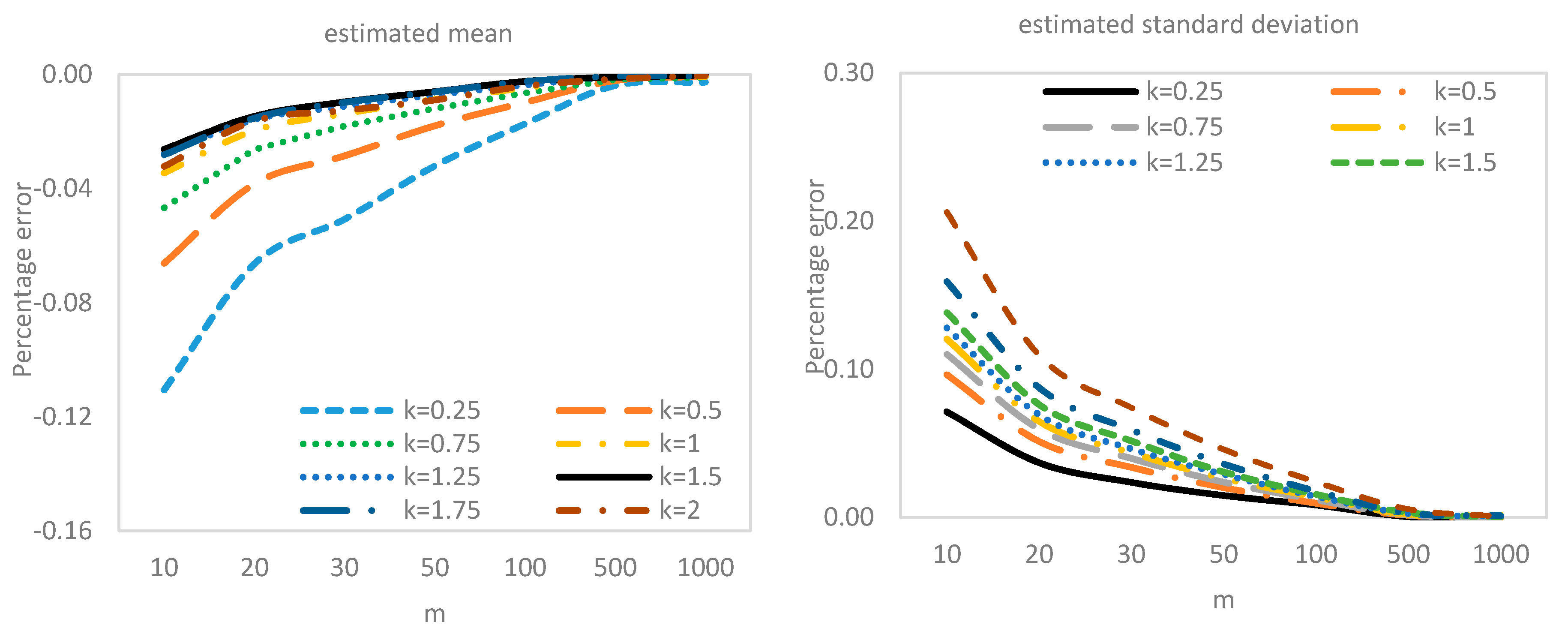
5.1. Performance Comparison with Respect to m
5.2. Performance Comparison with Respect to α
5.3. Performance Comparison with Respect to w
6. Illustrative Example
7. Practical Application
8. Conclusions
Author Contributions
Funding
Conflicts of Interest
Abbreviations
| CUSUM | Cumulative Sum |
| ARL | Average Run Length |
| SDRL | Standard Deviation of Run Length |
| RSS | Received Signal Strength |
| RL | Run Length |
| AR | Activity Recognition |
| AReM | Assembly Reliability Evaluation Method |
References
- Abujiya, M.a.R.; Riaz, M.; Lee, M.H. Enhanced cumulative sum charts for monitoring process dispersion. PLoS ONE 2015, 10, e0124520. [Google Scholar] [CrossRef] [PubMed]
- Page, E.S. Continuous inspection schemes. Biometrika 1954, 41, 100–114. [Google Scholar] [CrossRef]
- Montgomery, D.C. Introduction to Statistical Quality Control, 6th ed.; John Wiley & Sons: New York, NY, USA, 2009. [Google Scholar]
- Saleh, N.A.; Zwetsloot, I.M.; Mahmoud, M.A.; Woodall, W.H. CUSUM charts with controlled conditional performance under estimated parameters. Qual. Eng. 2016, 28, 402–415. [Google Scholar] [CrossRef]
- Schoonhoven, M.; Nazir, H.Z.; Riaz, M.; Does, R.J. Robust location estimators for the X-bar control chart. J. Qual. Technol. 2011, 48, 363–379. [Google Scholar] [CrossRef]
- Nazir, H.Z.; Riaz, M.; Does, R.J.M.M.; Abbas, N. Robust CUSUM control charting. Qual. Eng. 2013, 25, 211–224. [Google Scholar] [CrossRef]
- Amdouni, A.; Castagliola, P.; Taleb, H.; Celano, G. A variable sampling interval Shewhart control chart for monitoring the coefficient of variation in short production runs. Int. J. Prod. Res. 2017, 55, 5521–5536. [Google Scholar] [CrossRef]
- Abid, M.; Nazir, H.Z.; Riaz, M.; Lin, Z. Investigating the Impact of Ranked Set Sampling in Nonparametric CUSUM Control Charts. Qual. Reliab. Eng. Int. 2017, 33, 203–214. [Google Scholar] [CrossRef]
- Zhang, J.; Li, Z.; Chen, B.; Wang, Z. A new exponentially weighted moving average control chart for monitoring the coefficient of variation. Comput. Ind. Eng. 2014, 78, 205–212. [Google Scholar] [CrossRef]
- Mahmood, T.; Nazir, H.Z.; Abbas, N.; Riaz, M.; Ali, A. Performance evaluation of joint monitoring control charts. Sci. Iran. 2017, 24, 2152–2163. [Google Scholar] [CrossRef][Green Version]
- Hawkins, D.M. Identification of Outliers; Chapman and Hall: London, UK, 1980; Volume 11. [Google Scholar]
- Beckman, R.J.; Cook, R.D. Outlier … s. Technometrics 1983, 25, 119–149. [Google Scholar] [CrossRef]
- Barnett, V.; Lewis, T. Outliers in Statistical Data, 3rd ed.; John Wiley & Sons, Inc.: New York, NY, USA, 1994. [Google Scholar]
- Grubbs, F.E. Procedures for Detecting Outlying Observations in Samples. Technometrics 1969, 11, 1–21. [Google Scholar] [CrossRef]
- Tietjen, G.L.; Moore, R.H. Some Grubbs-Type Statistics for the Detection of Several Outliers. Technometrics 1972, 14, 583–597. [Google Scholar] [CrossRef]
- Lim, A.J.; Khoo, M.B.; Teoh, W.L.; Haq, A. Run sum chart for monitoring multivariate coefficient of variation. Comput. Ind. Eng. 2017, 109, 84–95. [Google Scholar] [CrossRef]
- Teoh, W.L.; Khoo, M.B.; Castagliola, P.; Yeong, W.C.; Teh, S.Y. Run-sum control charts for monitoring the coefficient of variation. Eur. J. Oper. Res. 2017, 257, 144–158. [Google Scholar] [CrossRef]
- Knorr, E.M.; Ng, R.T.; Tucakov, V. Distance-based outliers: Algorithms and applications. VLDB J. 2000, 8, 237–253. [Google Scholar] [CrossRef]
- Tse, Y.K.; Balasooriya, U. Tests for Multiple Outliers in an Exponential Sample. Indian J. Stat. Ser. B (1960–2002) 1991, 53, 56–63. [Google Scholar]
- Hubert, M.; Dierckx, G.; Vanpaemel, D. Detecting influential data points for the Hill estimator in Pareto-type distributions. Comput. Stat. Data Anal. 2013, 65, 13–28. [Google Scholar] [CrossRef]
- Castagliola, P.; Amdouni, A.; Taleb, H.; Celano, G. One-sided Shewhart-type charts for monitoring the coefficient of variation in short production runs. Qual. Technol. Quant. Manag. 2015, 12, 53–67. [Google Scholar] [CrossRef]
- Chen, G. The Mean and Standard Deviation of the Run Length Distribution of X Charts when Control Limits are Estimated. Stat. Sin. 1997, 7, 789–798. [Google Scholar]
- Mahmoud, M.A.; Henderson, G.R.; Epprecht, E.K.; Woodall, W.H. Estimating the Standard Deviation in Quality-Control Applications. J. Qual. Technol. 2010, 42, 348–357. [Google Scholar] [CrossRef]
- Nazir, H.Z.; Abbas, N.; Riaz, M.; Does, R.J.M.M. A comparative study of memory-type control charts under normal and contaminated normal environments. Qual. Reliab. Eng. Int. 2016, 32, 1347–1356. [Google Scholar] [CrossRef]
- Mahmood, T.; Xie, M. Models and monitoring of zero-inflated processes: The past and current trends. Qual. Reliab. Eng. Int. 2019, 35, 2540–2557. [Google Scholar] [CrossRef]
- Jones, L.A.; Champ, C.W.; Rigdon, S.E. The Run Length Distribution of the CUSUM with Estimated Parameters. J. Qual. Technol. 2004, 36, 95–108. [Google Scholar] [CrossRef]
- Dunbar, M.X. Analysis and Design of One-And Two-Sided CUSUM Charts with Known and Estimated Parameters. Master’s Thesis, Georgia Southern University, Statesboro, GA, USA, 2007. [Google Scholar]
- Tukey, J.W. Exploratory Data Analysis; Addison-Wesley: Boston, MA, USA, 1977. [Google Scholar]
- Kargupta, H.; Datta, S.; Wang, Q.; Sivakumar, K. Random-data Perturbation Techniques and Privacy-Preserving Data Mining. Knowl. Inf. Syst. 2005, 7, 387–414. [Google Scholar] [CrossRef]
- Liu, K.; Kargupta, H.; Ryan, J. Random Projection-based Multiplicative Data Perturbation for Privacy Preserving Distributed Data Mining. IEEE Trans. Knowl. Data Eng. 2006, 18, 92–106. [Google Scholar]
- Hong, E.P.; Kang, H.W.; Kang, C.W. DEWMA control chart for the coefficient of variation. In Proceedings of the Advanced Materials Research, Qinhuangdao, China, 28–31 October 2011; pp. 1682–1688. [Google Scholar]
- Du Nguyen, H.; Nguyen, Q.T.; Tran, K.P.; Ho, D.P. On the performance of VSI Shewhart control chart for monitoring the coefficient of variation in the presence of measurement errors. Int. J. Adv. Manuf. Technol. 2019, 104, 211–243. [Google Scholar] [CrossRef]
- Palumbo, F.; Gallicchio, C.; Pucci, R.; Micheli, A. Human Activity Recognition Using Multisensor Data Fusion Based on Reservoir Computing. J. Ambient Intell. Smart Environ. 2016, 8, 87–107. [Google Scholar] [CrossRef]


| Shewhart Chart | CUSUM | Robust CUSUM | Current Study | |
|---|---|---|---|---|
| Year | 1931 | 1954 | 2013 | 2020 |
| Author(s) | Shewhart W.A. | Page E.S. | Nazir et al. | Abbas et al. |
| Parameter of Interest | Process Mean | Process Mean | Process Mean | Process Mean |
| Plotting Statistic | Sample Mean | Cumulative sum of sample mean | Cumulative sum of robust estimators like sample median etc. | Cumulative sum of sample mean |
| Advantages |
|
|
|
|
| Disadvantages |
|
|
|
| k | h | RL Properties | δ | |||||||||
|---|---|---|---|---|---|---|---|---|---|---|---|---|
| 0.00 | 0.25 | 0.50 | 0.75 | 1.00 | 1.50 | 2.00 | 3.00 | 4.00 | 5.00 | |||
| 0.25 | 6.8516 | ARL | 200.000 | 63.588 | 24.229 | 14.076 | 9.862 | 6.195 | 4.558 | 3.060 | 2.328 | 2.013 |
| SDRL | 187.82 | 51.58 | 14.73 | 6.66 | 3.90 | 1.92 | 1.20 | 0.66 | 0.48 | 0.22 | ||
| 0.50 | 4.1713 | ARL | 199.997 | 83.100 | 28.438 | 13.921 | 8.724 | 4.918 | 3.456 | 2.259 | 1.772 | 1.372 |
| SDRL | 195.13 | 77.61 | 23.27 | 9.35 | 4.84 | 2.04 | 1.19 | 0.59 | 0.47 | 0.26 | ||
| 0.75 | 2.9332 | ARL | 200.008 | 102.897 | 37.458 | 16.792 | 9.446 | 4.641 | 3.063 | 1.898 | 1.381 | 1.094 |
| SDRL | 197.68 | 99.68 | 34.29 | 13.74 | 6.68 | 2.43 | 1.29 | 0.64 | 0.5 | 0.29 | ||
| 1.00 | 2.2137 | ARL | 200.006 | 119.968 | 48.841 | 21.705 | 11.406 | 4.864 | 2.956 | 1.695 | 1.219 | 1.037 |
| SDRL | 198.41 | 117.92 | 46.83 | 19.58 | 9.35 | 3.10 | 1.50 | 0.68 | 0.42 | 0.19 | ||
| m | k | h | RL Properties | δ | |||||||||
|---|---|---|---|---|---|---|---|---|---|---|---|---|---|
| 0.00 | 0.25 | 0.50 | 0.75 | 1.00 | 1.50 | 2.00 | 3.00 | 4.00 | 5.00 | ||||
| 10 | 0.25 | 7.609 | ARL | 199.383 | 104.343 | 33.241 | 16.709 | 11.229 | 6.884 | 5.019 | 3.343 | 2.551 | 2.093 |
| SDRL | 215.236 | 139.682 | 37.559 | 10.384 | 5.039 | 2.223 | 1.331 | 0.700 | 0.538 | 0.299 | |||
| 0.50 | 4.447 | ARL | 200.059 | 117.118 | 39.461 | 16.697 | 9.759 | 5.280 | 3.668 | 2.370 | 1.865 | 1.479 | |
| SDRL | 211.211 | 147.580 | 51.001 | 15.205 | 6.407 | 2.326 | 1.287 | 0.622 | 0.441 | 0.501 | |||
| 0.75 | 3.070 | ARL | 199.955 | 129.525 | 49.912 | 20.360 | 10.664 | 4.935 | 3.205 | 1.971 | 1.438 | 1.122 | |
| SDRL | 206.777 | 152.891 | 63.945 | 21.998 | 9.066 | 2.794 | 1.395 | 0.654 | 0.513 | 0.327 | |||
| 1.00 | 2.290 | ARL | 199.845 | 139.734 | 61.592 | 26.110 | 12.972 | 5.174 | 3.073 | 1.742 | 1.247 | 1.045 | |
| SDRL | 204.832 | 158.023 | 75.770 | 29.932 | 12.769 | 3.601 | 1.628 | 0.699 | 0.442 | 0.207 | |||
| 50 | 0.25 | 7.071 | ARL | 199.989 | 72.686 | 25.880 | 14.694 | 10.214 | 6.387 | 4.689 | 3.141 | 2.389 | 2.033 |
| SDRL | 191.101 | 70.530 | 17.200 | 7.228 | 4.108 | 1.985 | 1.228 | 0.669 | 0.505 | 0.230 | |||
| 0.50 | 4.246 | ARL | 200.328 | 91.515 | 30.404 | 14.476 | 8.958 | 5.010 | 3.510 | 2.289 | 1.799 | 1.401 | |
| SDRL | 196.721 | 94.950 | 27.139 | 10.218 | 5.097 | 2.101 | 1.208 | 0.595 | 0.462 | 0.491 | |||
| 0.75 | 2.968 | ARL | 200.300 | 109.736 | 39.790 | 17.480 | 9.687 | 4.709 | 3.097 | 1.916 | 1.396 | 1.100 | |
| SDRL | 198.429 | 113.866 | 39.054 | 15.037 | 7.057 | 2.504 | 1.309 | 0.643 | 0.502 | 0.300 | |||
| 1.00 | 2.233 | ARL | 200.129 | 125.358 | 51.433 | 22.548 | 11.722 | 4.928 | 2.983 | 1.706 | 1.226 | 1.039 | |
| SDRL | 199.137 | 128.594 | 52.200 | 21.314 | 9.944 | 3.184 | 1.526 | 0.683 | 0.427 | 0.193 | |||
| 100 | 0.25 | 6.970 | ARL | 199.946 | 68.273 | 25.057 | 14.395 | 10.048 | 6.297 | 4.627 | 3.104 | 2.360 | 2.024 |
| SDRL | 188.664 | 60.973 | 15.890 | 6.949 | 4.005 | 1.950 | 1.212 | 0.665 | 0.496 | 0.223 | |||
| 0.50 | 4.212 | ARL | 200.430 | 87.512 | 29.501 | 14.200 | 8.846 | 4.968 | 3.487 | 2.275 | 1.786 | 1.388 | |
| SDRL | 196.061 | 86.556 | 25.151 | 9.773 | 4.973 | 2.072 | 1.200 | 0.593 | 0.467 | 0.488 | |||
| 0.75 | 2.952 | ARL | 200.415 | 106.371 | 38.649 | 17.134 | 9.561 | 4.677 | 3.082 | 1.907 | 1.389 | 1.097 | |
| SDRL | 197.742 | 107.160 | 36.670 | 14.361 | 6.835 | 2.470 | 1.300 | 0.641 | 0.500 | 0.297 | |||
| 1.00 | 2.224 | ARL | 200.613 | 122.849 | 50.144 | 22.134 | 11.580 | 4.902 | 2.970 | 1.701 | 1.223 | 1.038 | |
| SDRL | 199.037 | 123.517 | 49.436 | 20.463 | 9.676 | 3.147 | 1.517 | 0.681 | 0.425 | 0.192 | |||
| 500 | 0.25 | 6.878 | ARL | 200.257 | 64.528 | 24.400 | 14.146 | 9.902 | 6.219 | 4.575 | 3.069 | 2.334 | 2.015 |
| SDRL | 187.975 | 53.602 | 14.933 | 6.715 | 3.917 | 1.927 | 1.201 | 0.662 | 0.486 | 0.220 | |||
| 0.50 | 4.180 | ARL | 200.348 | 83.934 | 28.700 | 13.981 | 8.748 | 4.925 | 3.464 | 2.262 | 1.775 | 1.374 | |
| SDRL | 195.114 | 79.434 | 23.596 | 9.440 | 4.861 | 2.047 | 1.190 | 0.589 | 0.470 | 0.485 | |||
| 0.75 | 2.938 | ARL | 200.330 | 103.981 | 37.728 | 16.880 | 9.480 | 4.650 | 3.067 | 1.900 | 1.383 | 1.095 | |
| SDRL | 197.702 | 101.518 | 34.763 | 13.883 | 6.700 | 2.445 | 1.293 | 0.640 | 0.498 | 0.294 | |||
| 1.00 | 2.215 | ARL | 199.622 | 120.377 | 49.084 | 21.814 | 11.427 | 4.867 | 2.957 | 1.695 | 1.221 | 1.037 | |
| SDRL | 197.769 | 119.228 | 47.308 | 19.817 | 9.394 | 3.105 | 1.503 | 0.678 | 0.423 | 0.189 | |||
| 1000 | 0.25 | 6.870 | ARL | 200.435 | 64.137 | 24.327 | 14.114 | 9.893 | 6.214 | 4.567 | 3.065 | 2.332 | 2.014 |
| SDRL | 187.977 | 52.723 | 14.812 | 6.680 | 3.920 | 1.921 | 1.197 | 0.661 | 0.485 | 0.220 | |||
| 0.50 | 4.174 | ARL | 199.921 | 83.373 | 28.488 | 13.939 | 8.729 | 4.923 | 3.460 | 2.260 | 1.773 | 1.372 | |
| SDRL | 195.128 | 78.425 | 23.332 | 9.391 | 4.837 | 2.049 | 1.189 | 0.589 | 0.471 | 0.484 | |||
| 0.75 | 2.936 | ARL | 200.261 | 103.481 | 37.557 | 16.832 | 9.456 | 4.644 | 3.066 | 1.900 | 1.382 | 1.095 | |
| SDRL | 197.588 | 100.857 | 34.560 | 13.811 | 6.670 | 2.434 | 1.292 | 0.641 | 0.498 | 0.293 | |||
| 1.00 | 2.215 | ARL | 200.364 | 120.208 | 48.942 | 21.746 | 11.422 | 4.870 | 2.959 | 1.695 | 1.220 | 1.038 | |
| SDRL | 198.748 | 118.622 | 46.945 | 19.748 | 9.394 | 3.107 | 1.505 | 0.679 | 0.423 | 0.190 | |||
| m | k | h | RL Properties | δ | |||||||||
|---|---|---|---|---|---|---|---|---|---|---|---|---|---|
| 0.00 | 0.25 | 0.50 | 0.75 | 1.00 | 1.50 | 2.00 | 3.00 | 4.00 | 5.00 | ||||
| 10 | 0.25 | 6.363 | ARL | 200.405 | 60.102 | 22.762 | 13.209 | 9.262 | 5.821 | 4.284 | 2.881 | 2.228 | 1.928 |
| SDRL | 307.837 | 58.830 | 15.242 | 6.830 | 4.001 | 1.990 | 1.258 | 0.712 | 0.473 | 0.347 | |||
| 0.50 | 3.769 | ARL | 200.186 | 79.654 | 26.646 | 12.915 | 8.080 | 4.554 | 3.205 | 2.103 | 1.611 | 1.256 | |
| SDRL | 373.977 | 116.713 | 27.155 | 9.947 | 5.004 | 2.089 | 1.210 | 0.626 | 0.521 | 0.437 | |||
| 0.75 | 2.610 | ARL | 200.504 | 101.344 | 35.910 | 15.787 | 8.789 | 4.289 | 2.826 | 1.741 | 1.279 | 1.063 | |
| SDRL | 404.643 | 185.346 | 50.475 | 16.502 | 7.323 | 2.518 | 1.321 | 0.662 | 0.458 | 0.244 | |||
| 1.00 | 1.947 | ARL | 199.994 | 119.320 | 47.933 | 20.909 | 10.796 | 4.528 | 2.734 | 1.568 | 1.162 | 1.026 | |
| SDRL | 419.821 | 241.979 | 82.668 | 27.810 | 11.547 | 3.348 | 1.557 | 0.671 | 0.377 | 0.159 | |||
| 50 | 0.25 | 6.750 | ARL | 200.033 | 62.844 | 23.946 | 13.890 | 9.733 | 6.116 | 4.504 | 3.021 | 2.307 | 2.000 |
| SDRL | 208.518 | 53.158 | 14.855 | 6.701 | 3.919 | 1.933 | 1.212 | 0.675 | 0.478 | 0.245 | |||
| 0.50 | 4.087 | ARL | 200.596 | 82.357 | 28.048 | 13.731 | 8.599 | 4.841 | 3.402 | 2.228 | 1.737 | 1.344 | |
| SDRL | 229.818 | 84.129 | 23.969 | 9.497 | 4.876 | 2.054 | 1.191 | 0.596 | 0.486 | 0.476 | |||
| 0.75 | 2.863 | ARL | 200.545 | 102.188 | 37.047 | 16.574 | 9.301 | 4.560 | 3.012 | 1.863 | 1.358 | 1.086 | |
| SDRL | 240.560 | 113.083 | 36.671 | 14.217 | 6.771 | 2.453 | 1.297 | 0.646 | 0.491 | 0.281 | |||
| 1.00 | 2.155 | ARL | 200.400 | 119.428 | 48.460 | 21.504 | 11.254 | 4.786 | 2.907 | 1.666 | 1.206 | 1.034 | |
| SDRL | 246.062 | 139.068 | 51.874 | 20.928 | 9.711 | 3.141 | 1.514 | 0.678 | 0.413 | 0.182 | |||
| 100 | 0.25 | 6.794 | ARL | 199.294 | 63.155 | 24.052 | 13.966 | 9.786 | 6.154 | 4.526 | 3.037 | 2.316 | 2.006 |
| SDRL | 197.077 | 52.484 | 14.746 | 6.675 | 3.906 | 1.927 | 1.206 | 0.668 | 0.480 | 0.232 | |||
| 0.50 | 4.131 | ARL | 200.578 | 82.766 | 28.225 | 13.823 | 8.652 | 4.884 | 3.431 | 2.244 | 1.755 | 1.359 | |
| SDRL | 212.753 | 80.763 | 23.573 | 9.417 | 4.841 | 2.051 | 1.189 | 0.593 | 0.479 | 0.480 | |||
| 0.75 | 2.898 | ARL | 200.473 | 102.694 | 37.300 | 16.685 | 9.375 | 4.607 | 3.037 | 1.880 | 1.370 | 1.090 | |
| SDRL | 218.562 | 106.845 | 35.484 | 13.983 | 6.724 | 2.450 | 1.294 | 0.643 | 0.494 | 0.287 | |||
| 1.00 | 2.183 | ARL | 199.677 | 119.568 | 48.559 | 21.547 | 11.325 | 4.824 | 2.929 | 1.680 | 1.212 | 1.035 | |
| SDRL | 220.710 | 127.965 | 49.291 | 20.189 | 9.534 | 3.126 | 1.506 | 0.678 | 0.417 | 0.185 | |||
| 500 | 0.25 | 6.848 | ARL | 200.572 | 63.552 | 24.226 | 14.080 | 9.862 | 6.193 | 4.557 | 3.059 | 2.328 | 2.013 |
| SDRL | 190.749 | 51.951 | 14.746 | 6.675 | 3.904 | 1.923 | 1.200 | 0.663 | 0.483 | 0.222 | |||
| 0.50 | 4.165 | ARL | 200.223 | 83.177 | 28.415 | 13.913 | 8.707 | 4.914 | 3.453 | 2.257 | 1.769 | 1.369 | |
| SDRL | 198.681 | 78.455 | 23.301 | 9.377 | 4.831 | 2.049 | 1.189 | 0.590 | 0.473 | 0.483 | |||
| 0.75 | 2.928 | ARL | 200.675 | 103.041 | 37.404 | 16.783 | 9.438 | 4.635 | 3.060 | 1.894 | 1.380 | 1.093 | |
| SDRL | 201.922 | 101.276 | 34.557 | 13.773 | 6.672 | 2.436 | 1.293 | 0.641 | 0.497 | 0.291 | |||
| 1.00 | 2.209 | ARL | 200.376 | 120.019 | 48.878 | 21.737 | 11.392 | 4.860 | 2.951 | 1.693 | 1.219 | 1.036 | |
| SDRL | 203.135 | 120.335 | 47.389 | 19.798 | 9.403 | 3.108 | 1.500 | 0.678 | 0.421 | 0.187 | |||
| 1000 | 0.25 | 6.851 | ARL | 200.377 | 63.648 | 24.239 | 14.082 | 9.862 | 6.196 | 4.558 | 3.059 | 2.328 | 2.013 |
| SDRL | 189.279 | 52.107 | 14.755 | 6.672 | 3.897 | 1.920 | 1.200 | 0.662 | 0.484 | 0.221 | |||
| 0.50 | 4.171 | ARL | 201.035 | 83.254 | 28.515 | 13.940 | 8.726 | 4.918 | 3.455 | 2.258 | 1.772 | 1.372 | |
| SDRL | 197.398 | 78.294 | 23.316 | 9.384 | 4.844 | 2.045 | 1.186 | 0.589 | 0.471 | 0.484 | |||
| 0.75 | 2.933 | ARL | 200.892 | 103.327 | 37.531 | 16.820 | 9.435 | 4.644 | 3.063 | 1.898 | 1.381 | 1.094 | |
| SDRL | 200.377 | 100.860 | 34.491 | 13.805 | 6.655 | 2.440 | 1.291 | 0.640 | 0.497 | 0.292 | |||
| 1.00 | 2.210 | ARL | 199.787 | 120.041 | 48.756 | 21.688 | 11.387 | 4.859 | 2.956 | 1.694 | 1.218 | 1.037 | |
| SDRL | 199.806 | 119.231 | 47.036 | 19.668 | 9.374 | 3.104 | 1.506 | 0.678 | 0.421 | 0.189 | |||
| m | k | h | RL Properties | δ | |||||||||
|---|---|---|---|---|---|---|---|---|---|---|---|---|---|
| 0.00 | 0.25 | 0.50 | 0.75 | 1.00 | 1.50 | 2.00 | 3.00 | 4.00 | 5.00 | ||||
| 10 | 0.25 | 7.059 | ARL | 199.839 | 102.365 | 31.358 | 15.661 | 10.522 | 6.458 | 4.716 | 3.143 | 2.408 | 2.036 |
| SDRL | 343.854 | 200.559 | 42.962 | 10.656 | 5.112 | 2.294 | 1.399 | 0.762 | 0.538 | 0.334 | |||
| 0.50 | 4.010 | ARL | 200.741 | 115.384 | 37.440 | 15.548 | 9.038 | 4.874 | 3.392 | 2.204 | 1.700 | 1.333 | |
| SDRL | 403.561 | 253.069 | 72.922 | 17.311 | 6.674 | 2.360 | 1.308 | 0.649 | 0.515 | 0.473 | |||
| 0.75 | 2.719 | ARL | 199.462 | 128.278 | 48.250 | 19.298 | 9.906 | 4.551 | 2.945 | 1.801 | 1.319 | 1.080 | |
| SDRL | 428.983 | 293.013 | 104.853 | 28.936 | 10.291 | 2.891 | 1.420 | 0.681 | 0.480 | 0.272 | |||
| 1.00 | 2.010 | ARL | 200.078 | 139.638 | 60.751 | 25.381 | 12.370 | 4.810 | 2.837 | 1.607 | 1.181 | 1.031 | |
| SDRL | 444.178 | 321.987 | 137.963 | 46.283 | 17.357 | 3.932 | 1.684 | 0.694 | 0.396 | 0.174 | |||
| 50 | 0.25 | 6.917 | ARL | 199.699 | 67.771 | 24.906 | 14.312 | 9.989 | 6.255 | 4.601 | 3.085 | 2.348 | 2.019 |
| SDRL | 198.389 | 61.666 | 15.955 | 6.957 | 4.018 | 1.962 | 1.222 | 0.671 | 0.493 | 0.233 | |||
| 0.50 | 4.169 | ARL | 200.336 | 87.245 | 29.240 | 14.097 | 8.774 | 4.924 | 3.462 | 2.259 | 1.769 | 1.373 | |
| SDRL | 212.799 | 90.310 | 25.530 | 9.843 | 4.987 | 2.078 | 1.203 | 0.595 | 0.475 | 0.484 | |||
| 0.75 | 2.913 | ARL | 199.648 | 105.684 | 38.333 | 16.994 | 9.493 | 4.631 | 3.053 | 1.889 | 1.376 | 1.093 | |
| SDRL | 217.876 | 113.732 | 37.851 | 14.602 | 6.933 | 2.478 | 1.304 | 0.646 | 0.496 | 0.291 | |||
| 1.00 | 2.193 | ARL | 199.956 | 122.288 | 49.919 | 22.003 | 11.479 | 4.851 | 2.946 | 1.685 | 1.215 | 1.037 | |
| SDRL | 221.744 | 133.825 | 52.081 | 21.110 | 9.823 | 3.163 | 1.520 | 0.680 | 0.420 | 0.188 | |||
| 100 | 0.25 | 6.917 | ARL | 199.699 | 67.771 | 24.906 | 14.312 | 9.989 | 6.255 | 4.601 | 3.085 | 2.348 | 2.019 |
| SDRL | 198.389 | 61.666 | 15.955 | 6.957 | 4.018 | 1.962 | 1.222 | 0.671 | 0.493 | 0.233 | |||
| 0.50 | 4.169 | ARL | 200.336 | 87.245 | 29.240 | 14.097 | 8.774 | 4.924 | 3.462 | 2.259 | 1.769 | 1.373 | |
| SDRL | 212.799 | 90.310 | 25.530 | 9.843 | 4.987 | 2.078 | 1.203 | 0.595 | 0.475 | 0.484 | |||
| 0.75 | 2.913 | ARL | 199.648 | 105.684 | 38.333 | 16.994 | 9.493 | 4.631 | 3.053 | 1.889 | 1.376 | 1.093 | |
| SDRL | 217.876 | 113.732 | 37.851 | 14.602 | 6.933 | 2.478 | 1.304 | 0.646 | 0.496 | 0.291 | |||
| 1.00 | 2.193 | ARL | 199.956 | 122.288 | 49.919 | 22.003 | 11.479 | 4.851 | 2.946 | 1.685 | 1.215 | 1.037 | |
| SDRL | 221.744 | 133.825 | 52.081 | 21.110 | 9.823 | 3.163 | 1.520 | 0.680 | 0.420 | 0.188 | |||
| 500 | 0.25 | 6.868 | ARL | 199.857 | 64.355 | 24.398 | 14.122 | 9.885 | 6.210 | 4.566 | 3.067 | 2.332 | 2.014 |
| SDRL | 189.936 | 53.531 | 15.008 | 6.715 | 3.920 | 1.926 | 1.201 | 0.663 | 0.485 | 0.222 | |||
| 0.50 | 4.171 | ARL | 200.044 | 83.865 | 28.607 | 13.953 | 8.734 | 4.921 | 3.457 | 2.260 | 1.770 | 1.372 | |
| SDRL | 198.638 | 80.168 | 23.684 | 9.432 | 4.865 | 2.049 | 1.190 | 0.589 | 0.472 | 0.484 | |||
| 0.75 | 2.930 | ARL | 200.139 | 103.405 | 37.595 | 16.856 | 9.462 | 4.637 | 3.063 | 1.896 | 1.380 | 1.094 | |
| SDRL | 201.232 | 102.432 | 34.956 | 13.942 | 6.707 | 2.443 | 1.294 | 0.641 | 0.497 | 0.292 | |||
| 1.00 | 2.209 | ARL | 199.771 | 120.239 | 48.995 | 21.793 | 11.431 | 4.859 | 2.953 | 1.694 | 1.218 | 1.037 | |
| SDRL | 202.617 | 120.900 | 47.734 | 19.947 | 9.460 | 3.105 | 1.505 | 0.679 | 0.421 | 0.189 | |||
| 1000 | 0.25 | 6.860 | ARL | 199.887 | 63.963 | 24.302 | 14.097 | 9.870 | 6.205 | 4.563 | 3.063 | 2.330 | 2.014 |
| SDRL | 188.749 | 52.600 | 14.842 | 6.692 | 3.908 | 1.924 | 1.201 | 0.661 | 0.484 | 0.221 | |||
| 0.50 | 4.172 | ARL | 200.175 | 83.432 | 28.542 | 13.943 | 8.728 | 4.917 | 3.458 | 2.260 | 1.772 | 1.372 | |
| SDRL | 196.712 | 78.731 | 23.482 | 9.400 | 4.849 | 2.046 | 1.190 | 0.589 | 0.472 | 0.484 | |||
| 0.75 | 2.933 | ARL | 200.433 | 103.187 | 37.606 | 16.838 | 9.465 | 4.642 | 3.063 | 1.898 | 1.382 | 1.094 | |
| SDRL | 199.533 | 101.221 | 34.688 | 13.848 | 6.697 | 2.439 | 1.292 | 0.640 | 0.498 | 0.292 | |||
| 1.00 | 2.213 | ARL | 200.351 | 120.455 | 49.060 | 21.776 | 11.414 | 4.866 | 2.958 | 1.695 | 1.219 | 1.037 | |
| SDRL | 201.344 | 120.017 | 47.496 | 19.808 | 9.407 | 3.109 | 1.505 | 0.679 | 0.422 | 0.189 | |||
| µ | σ | m | k | |||||||
|---|---|---|---|---|---|---|---|---|---|---|
| 0.25 | 0.50 | 0.75 | 1.00 | 1.25 | 1.50 | 1.75 | 2.00 | |||
| known | known | - | 6.852 | 4.171 | 2.933 | 2.214 | 1.741 | 1.387 | 1.089 | 0.819 |
| estimated | known | 10 | 7.609 | 4.447 | 3.070 | 2.290 | 1.789 | 1.423 | 1.120 | 0.845 |
| 20 | 7.306 | 4.331 | 3.010 | 2.257 | 1.768 | 1.407 | 1.106 | 0.832 | ||
| 30 | 7.199 | 4.290 | 2.986 | 2.244 | 1.760 | 1.400 | 1.100 | 0.829 | ||
| 50 | 7.071 | 4.246 | 2.968 | 2.233 | 1.753 | 1.395 | 1.096 | 0.826 | ||
| 100 | 6.970 | 4.212 | 2.952 | 2.224 | 1.747 | 1.390 | 1.092 | 0.822 | ||
| 500 | 6.878 | 4.180 | 2.938 | 2.215 | 1.742 | 1.388 | 1.090 | 0.820 | ||
| 1000 | 6.870 | 4.174 | 2.936 | 2.215 | 1.741 | 1.387 | 1.090 | 0.819 | ||
| known | estimated | 10 | 6.363 | 3.769 | 2.610 | 1.947 | 1.518 | 1.195 | 0.916 | 0.650 |
| 20 | 6.598 | 3.957 | 2.758 | 2.070 | 1.620 | 1.281 | 0.994 | 0.729 | ||
| 30 | 6.689 | 4.030 | 2.816 | 2.117 | 1.660 | 1.315 | 1.025 | 0.758 | ||
| 50 | 6.750 | 4.087 | 2.863 | 2.155 | 1.690 | 1.344 | 1.050 | 0.781 | ||
| 100 | 6.794 | 4.131 | 2.898 | 2.183 | 1.716 | 1.365 | 1.070 | 0.799 | ||
| 500 | 6.848 | 4.165 | 2.928 | 2.209 | 1.736 | 1.382 | 1.086 | 0.814 | ||
| 1000 | 6.851 | 4.171 | 2.933 | 2.210 | 1.739 | 1.386 | 1.088 | 0.818 | ||
| estimated | estimated | 10 | 7.059 | 4.010 | 2.719 | 2.010 | 1.557 | 1.223 | 0.938 | 0.672 |
| 20 | 7.051 | 4.110 | 2.827 | 2.107 | 1.645 | 1.299 | 1.009 | 0.743 | ||
| 30 | 7.019 | 4.140 | 2.866 | 2.144 | 1.675 | 1.328 | 1.035 | 0.768 | ||
| 50 | 6.973 | 4.159 | 2.896 | 2.171 | 1.701 | 1.352 | 1.057 | 0.788 | ||
| 100 | 6.917 | 4.169 | 2.913 | 2.193 | 1.721 | 1.370 | 1.074 | 0.804 | ||
| 500 | 6.868 | 4.171 | 2.930 | 2.209 | 1.737 | 1.384 | 1.086 | 0.815 | ||
| 1000 | 6.860 | 4.172 | 2.933 | 2.213 | 1.740 | 1.386 | 1.088 | 0.818 | ||
| m | k | h | RL Properties | w = 1 | w = 2 | w = 3 | ||||||||||||
|---|---|---|---|---|---|---|---|---|---|---|---|---|---|---|---|---|---|---|
| α | α | α | ||||||||||||||||
| 0.00 | 0.01 | 0.02 | 0.03 | 0.04 | 0.00 | 0.01 | 0.02 | 0.03 | 0.04 | 0.00 | 0.01 | 0.02 | 0.03 | 0.04 | ||||
| 10 | 0.25 | 7.609 | ARL | 199 | 198 | 196 | 194 | 192 | 199 | 195 | 190 | 182 | 178 | 199 | 192 | 183 | 173 | 163 |
| SDRL | 215 | 214 | 213 | 212 | 212 | 215 | 213 | 211 | 206 | 205 | 215 | 213 | 208 | 204 | 198 | |||
| 0.50 | 4.447 | ARL | 200 | 199 | 198 | 196 | 195 | 200 | 195 | 191 | 187 | 180 | 200 | 194 | 185 | 177 | 167 | |
| SDRL | 211 | 210 | 211 | 210 | 209 | 211 | 209 | 206 | 206 | 200 | 211 | 210 | 204 | 201 | 196 | |||
| 0.75 | 3.070 | ARL | 200 | 199 | 199 | 198 | 196 | 200 | 198 | 194 | 189 | 184 | 200 | 193 | 187 | 179 | 171 | |
| SDRL | 207 | 207 | 207 | 206 | 207 | 207 | 206 | 204 | 203 | 198 | 207 | 203 | 202 | 198 | 193 | |||
| 1.00 | 2.290 | ARL | 200 | 199 | 198 | 197 | 196 | 200 | 197 | 195 | 189 | 186 | 200 | 195 | 189 | 182 | 176 | |
| SDRL | 205 | 203 | 204 | 202 | 202 | 205 | 202 | 202 | 198 | 196 | 205 | 201 | 199 | 195 | 191 | |||
| 50 | 0.25 | 7.071 | ARL | 200 | 198 | 197 | 194 | 192 | 200 | 197 | 190 | 181 | 169 | 200 | 192 | 179 | 164 | 147 |
| SDRL | 191 | 189 | 190 | 187 | 186 | 191 | 189 | 184 | 177 | 169 | 191 | 187 | 177 | 166 | 154 | |||
| 0.50 | 4.246 | ARL | 200 | 199 | 198 | 196 | 194 | 200 | 197 | 192 | 186 | 178 | 200 | 194 | 186 | 172 | 158 | |
| SDRL | 197 | 195 | 195 | 194 | 192 | 197 | 195 | 191 | 186 | 179 | 197 | 193 | 185 | 176 | 165 | |||
| 0.75 | 2.968 | ARL | 200 | 199 | 199 | 198 | 195 | 200 | 198 | 195 | 189 | 184 | 200 | 196 | 188 | 179 | 167 | |
| SDRL | 198 | 197 | 198 | 197 | 195 | 198 | 198 | 195 | 190 | 185 | 198 | 195 | 189 | 182 | 172 | |||
| 1.00 | 2.233 | ARL | 200 | 200 | 199 | 199 | 197 | 200 | 198 | 195 | 192 | 188 | 200 | 197 | 191 | 183 | 174 | |
| SDRL | 199 | 199 | 198 | 198 | 196 | 199 | 197 | 195 | 191 | 190 | 199 | 196 | 192 | 186 | 177 | |||
| 100 | 0.25 | 6.97 | ARL | 200 | 199 | 197 | 195 | 191 | 200 | 196 | 189 | 180 | 168 | 200 | 193 | 178 | 161 | 141 |
| SDRL | 189 | 188 | 186 | 185 | 180 | 189 | 187 | 179 | 172 | 163 | 189 | 183 | 172 | 159 | 142 | |||
| 0.50 | 4.212 | ARL | 200 | 200 | 200 | 196 | 195 | 200 | 198 | 193 | 187 | 177 | 200 | 196 | 185 | 173 | 156 | |
| SDRL | 196 | 196 | 196 | 192 | 192 | 196 | 193 | 189 | 185 | 176 | 196 | 192 | 183 | 173 | 158 | |||
| 0.75 | 2.952 | ARL | 200 | 201 | 199 | 197 | 196 | 200 | 200 | 194 | 191 | 185 | 200 | 196 | 189 | 178 | 168 | |
| SDRL | 198 | 199 | 197 | 195 | 195 | 198 | 196 | 192 | 189 | 184 | 198 | 195 | 189 | 178 | 168 | |||
| 1.00 | 2.224 | ARL | 201 | 199 | 201 | 199 | 197 | 201 | 199 | 196 | 194 | 188 | 201 | 199 | 192 | 185 | 173 | |
| SDRL | 199 | 198 | 200 | 197 | 197 | 199 | 197 | 195 | 193 | 188 | 199 | 198 | 192 | 185 | 174 | |||
| 500 | 0.25 | 6.878 | ARL | 200 | 199 | 197 | 195 | 189 | 200 | 196 | 189 | 177 | 164 | 200 | 194 | 179 | 156 | 134 |
| SDRL | 188 | 187 | 187 | 183 | 178 | 188 | 184 | 177 | 166 | 154 | 188 | 181 | 168 | 146 | 126 | |||
| 0.50 | 4.18 | ARL | 200 | 201 | 199 | 197 | 193 | 200 | 199 | 192 | 186 | 175 | 200 | 196 | 185 | 171 | 153 | |
| SDRL | 195 | 195 | 194 | 192 | 189 | 195 | 193 | 188 | 181 | 172 | 195 | 191 | 181 | 167 | 151 | |||
| 0.75 | 2.938 | ARL | 200 | 201 | 199 | 197 | 195 | 200 | 200 | 195 | 190 | 183 | 200 | 198 | 191 | 180 | 166 | |
| SDRL | 198 | 198 | 196 | 195 | 193 | 198 | 197 | 193 | 187 | 180 | 198 | 195 | 190 | 179 | 164 | |||
| 1.00 | 2.215 | ARL | 200 | 200 | 199 | 199 | 196 | 200 | 198 | 197 | 192 | 188 | 200 | 198 | 193 | 185 | 174 | |
| SDRL | 198 | 199 | 197 | 197 | 193 | 198 | 196 | 196 | 190 | 185 | 198 | 196 | 191 | 182 | 173 | |||
| 1000 | 0.25 | 6.870 | ARL | 200 | 201 | 198 | 193 | 190 | 200 | 198 | 190 | 178 | 163 | 200 | 194 | 178 | 156 | 134 |
| SDRL | 188 | 189 | 186 | 181 | 179 | 188 | 186 | 178 | 166 | 153 | 188 | 182 | 167 | 144 | 124 | |||
| 0.50 | 4.174 | ARL | 200 | 200 | 198 | 197 | 194 | 200 | 198 | 193 | 186 | 176 | 200 | 196 | 185 | 171 | 153 | |
| SDRL | 195 | 195 | 193 | 191 | 189 | 195 | 193 | 188 | 181 | 171 | 195 | 190 | 180 | 167 | 149 | |||
| 0.75 | 2.936 | ARL | 200 | 199 | 199 | 197 | 196 | 200 | 200 | 197 | 191 | 183 | 200 | 198 | 191 | 179 | 166 | |
| SDRL | 198 | 195 | 197 | 194 | 194 | 198 | 198 | 194 | 189 | 180 | 198 | 195 | 189 | 175 | 165 | |||
| 1.00 | 2.215 | ARL | 200 | 199 | 200 | 198 | 198 | 200 | 200 | 198 | 192 | 188 | 200 | 198 | 192 | 185 | 173 | |
| SDRL | 199 | 199 | 199 | 196 | 197 | 199 | 198 | 195 | 190 | 186 | 199 | 196 | 191 | 183 | 172 | |||
| m | k | h | RL Properties | w = 1 | w = 2 | w = 3 | ||||||||||||
|---|---|---|---|---|---|---|---|---|---|---|---|---|---|---|---|---|---|---|
| α | α | α | ||||||||||||||||
| 0.00 | 0.01 | 0.02 | 0.03 | 0.04 | 0.00 | 0.01 | 0.02 | 0.03 | 0.04 | 0.00 | 0.01 | 0.02 | 0.03 | 0.04 | ||||
| 10 | 0.25 | 6.363 | ARL | 200 | 232 | 271 | 308 | 369 | 200 | 1252 | 2827 | 5180 | 7632 | 200 | 5766 | 13,029 | 22,028 | 33,346 |
| SDRL | 308 | 720 | 1271 | 1442 | 2202 | 308 | 25,588 | 41,781 | 59,472 | 72,550 | 308 | 66,775 | 101,057 | 131,849 | 163,026 | |||
| 0.50 | 3.769 | ARL | 200 | 253 | 320 | 402 | 498 | 200 | 2374 | 5025 | 8677 | 13,606 | 200 | 8574 | 19,938 | 32,755 | 49,639 | |
| SDRL | 374 | 1216 | 1839 | 2660 | 3384 | 374 | 39,571 | 59,416 | 79,131 | 100,612 | 374 | 82,482 | 127,093 | 162,747 | 200,013 | |||
| 0.75 | 2.610 | ARL | 201 | 266 | 374 | 471 | 569 | 201 | 2614 | 6115 | 10,306 | 15,478 | 201 | 10,440 | 23,698 | 39,039 | 56,370 | |
| SDRL | 405 | 1397 | 2665 | 3349 | 3891 | 405 | 41,686 | 66,631 | 86,598 | 107,915 | 405 | 92,015 | 139,038 | 178,484 | 213,382 | |||
| 1.00 | 1.947 | ARL | 200 | 289 | 386 | 484 | 599 | 200 | 3152 | 6751 | 10,527 | 16,605 | 200 | 10,322 | 24,092 | 40,720 | 59,187 | |
| SDRL | 420 | 1851 | 2745 | 3539 | 4090 | 420 | 46,733 | 69,185 | 87,750 | 111,809 | 420 | 91,131 | 140,118 | 181,993 | 218,900 | |||
| 50 | 0.25 | 6.750 | ARL | 200 | 213 | 229 | 245 | 262 | 200 | 249 | 313 | 399 | 522 | 200 | 320 | 598 | 1020 | 2048 |
| SDRL | 209 | 225 | 249 | 271 | 298 | 209 | 304 | 455 | 892 | 1381 | 209 | 958 | 6844 | 9008 | 19,563 | |||
| 0.50 | 4.087 | ARL | 201 | 220 | 240 | 263 | 287 | 201 | 274 | 377 | 550 | 767 | 201 | 413 | 1043 | 2332 | 5481 | |
| SDRL | 230 | 259 | 294 | 328 | 379 | 230 | 453 | 1093 | 4144 | 4185 | 230 | 2854 | 11,610 | 24,597 | 45,072 | |||
| 0.75 | 2.863 | ARL | 201 | 221 | 245 | 272 | 299 | 201 | 288 | 425 | 614 | 970 | 201 | 499 | 1284 | 3489 | 7734 | |
| SDRL | 241 | 274 | 314 | 379 | 417 | 241 | 655 | 1509 | 2443 | 7384 | 241 | 5406 | 14,261 | 32,417 | 56,026 | |||
| 1.00 | 2.155 | ARL | 200 | 223 | 248 | 275 | 309 | 200 | 295 | 453 | 713 | 1113 | 200 | 517 | 1622 | 3965 | 9219 | |
| SDRL | 246 | 285 | 340 | 383 | 450 | 246 | 628 | 3646 | 5086 | 8738 | 246 | 5297 | 19,603 | 35,460 | 63,990 | |||
| 100 | 0.25 | 6.794 | ARL | 199 | 212 | 226 | 242 | 257 | 199 | 240 | 294 | 360 | 440 | 199 | 284 | 416 | 621 | 984 |
| SDRL | 197 | 210 | 229 | 246 | 266 | 197 | 250 | 329 | 427 | 573 | 197 | 334 | 636 | 1439 | 2903 | |||
| 0.50 | 4.131 | ARL | 201 | 218 | 237 | 258 | 281 | 201 | 258 | 335 | 437 | 582 | 201 | 333 | 555 | 1005 | 1883 | |
| SDRL | 213 | 235 | 258 | 284 | 315 | 213 | 301 | 428 | 616 | 953 | 213 | 1159 | 1079 | 5010 | 9240 | |||
| 0.75 | 2.898 | ARL | 200 | 221 | 243 | 265 | 292 | 200 | 267 | 358 | 494 | 671 | 200 | 351 | 649 | 1290 | 2600 | |
| SDRL | 219 | 244 | 276 | 302 | 338 | 219 | 330 | 495 | 799 | 1297 | 219 | 586 | 2578 | 7319 | 14,579 | |||
| 1.00 | 2.183 | ARL | 200 | 221 | 242 | 270 | 295 | 200 | 269 | 376 | 517 | 718 | 200 | 360 | 700 | 1417 | 3124 | |
| SDRL | 221 | 249 | 277 | 321 | 349 | 221 | 340 | 555 | 948 | 1354 | 221 | 595 | 2335 | 6141 | 18,020 | |||
| 500 | 0.25 | 6.848 | ARL | 201 | 213 | 227 | 242 | 257 | 201 | 238 | 284 | 340 | 411 | 201 | 272 | 375 | 523 | 735 |
| SDRL | 191 | 203 | 218 | 232 | 248 | 191 | 228 | 278 | 337 | 412 | 191 | 267 | 381 | 550 | 807 | |||
| 0.50 | 4.165 | ARL | 200 | 218 | 237 | 255 | 276 | 200 | 251 | 317 | 399 | 510 | 200 | 298 | 454 | 702 | 1098 | |
| SDRL | 199 | 216 | 236 | 256 | 280 | 199 | 253 | 326 | 416 | 543 | 199 | 306 | 492 | 796 | 1317 | |||
| 0.75 | 2.928 | ARL | 201 | 218 | 240 | 261 | 286 | 201 | 257 | 333 | 435 | 565 | 201 | 315 | 499 | 814 | 1350 | |
| SDRL | 202 | 221 | 243 | 265 | 292 | 202 | 264 | 347 | 463 | 613 | 202 | 330 | 554 | 963 | 1698 | |||
| 1.00 | 2.209 | ARL | 200 | 219 | 241 | 264 | 291 | 200 | 261 | 343 | 455 | 597 | 200 | 321 | 527 | 882 | 1509 | |
| SDRL | 203 | 222 | 247 | 272 | 298 | 203 | 269 | 361 | 488 | 652 | 203 | 341 | 595 | 1052 | 1921 | |||
| 1000 | 0.25 | 6.851 | ARL | 200 | 214 | 227 | 240 | 256 | 200 | 237 | 284 | 339 | 405 | 200 | 269 | 368 | 514 | 717 |
| SDRL | 189 | 203 | 216 | 228 | 244 | 189 | 227 | 273 | 330 | 401 | 189 | 260 | 362 | 517 | 740 | |||
| 0.50 | 4.171 | ARL | 201 | 219 | 235 | 254 | 277 | 201 | 251 | 313 | 396 | 501 | 201 | 295 | 445 | 681 | 1058 | |
| SDRL | 197 | 216 | 233 | 251 | 277 | 197 | 249 | 314 | 402 | 512 | 197 | 298 | 457 | 726 | 1138 | |||
| 0.75 | 2.933 | ARL | 201 | 220 | 240 | 262 | 285 | 201 | 258 | 332 | 432 | 558 | 201 | 311 | 490 | 784 | 1280 | |
| SDRL | 200 | 220 | 240 | 263 | 288 | 200 | 259 | 338 | 442 | 578 | 200 | 318 | 516 | 840 | 1420 | |||
| 1.00 | 2.210 | ARL | 200 | 219 | 242 | 265 | 289 | 200 | 261 | 340 | 446 | 586 | 200 | 317 | 511 | 844 | 1408 | |
| SDRL | 200 | 221 | 244 | 267 | 290 | 200 | 264 | 349 | 460 | 612 | 200 | 329 | 542 | 911 | 1580 | |||
| m | k | h | RL Properties | w = 1 | w = 2 | w = 3 | ||||||||||||
|---|---|---|---|---|---|---|---|---|---|---|---|---|---|---|---|---|---|---|
| α | α | α | ||||||||||||||||
| 0.00 | 0.01 | 0.02 | 0.03 | 0.04 | 0.00 | 0.01 | 0.02 | 0.03 | 0.04 | 0.00 | 0.01 | 0.02 | 0.03 | 0.04 | ||||
| 10 | 0.25 | 7.059 | ARL | 200 | 220 | 238 | 257 | 264 | 200 | 289 | 420 | 506 | 522 | 200 | 415 | 667 | 834 | 1018 |
| SDRL | 344 | 579 | 802 | 1325 | 880 | 344 | 2389 | 8400 | 8836 | 7702 | 344 | 6970 | 12,597 | 13,937 | 15,538 | |||
| 0.50 | 4.010 | ARL | 201 | 244 | 315 | 333 | 390 | 201 | 691 | 1221 | 2017 | 2556 | 201 | 2465 | 4835 | 7722 | 10,719 | |
| SDRL | 404 | 1375 | 5270 | 4092 | 5614 | 404 | 15,507 | 21,367 | 30,537 | 34,157 | 404 | 38,100 | 54,564 | 70,640 | 84,741 | |||
| 0.75 | 2.719 | ARL | 199 | 291 | 340 | 409 | 497 | 199 | 1402 | 2839 | 4258 | 6234 | 199 | 4856 | 10,452 | 18,230 | 25,507 | |
| SDRL | 429 | 5091 | 5290 | 5868 | 8207 | 429 | 27,821 | 40,327 | 50,689 | 62,254 | 429 | 58,258 | 87,142 | 116,950 | 139,084 | |||
| 1.00 | 2.010 | ARL | 200 | 280 | 396 | 468 | 642 | 200 | 1919 | 3740 | 6103 | 8942 | 200 | 7038 | 15,601 | 24,673 | 35,470 | |
| SDRL | 444 | 2471 | 7494 | 7088 | 11,812 | 444 | 33,960 | 48,185 | 62,320 | 77,490 | 444 | 72,692 | 109,882 | 138,233 | 165,823 | |||
| 50 | 0.25 | 6.917 | ARL | 201 | 212 | 227 | 233 | 242 | 201 | 238 | 268 | 297 | 319 | 201 | 265 | 323 | 366 | 391 |
| SDRL | 212 | 228 | 250 | 259 | 270 | 212 | 276 | 331 | 381 | 429 | 212 | 355 | 474 | 560 | 616 | |||
| 0.50 | 4.169 | ARL | 201 | 218 | 236 | 253 | 271 | 201 | 260 | 326 | 405 | 482 | 201 | 333 | 495 | 715 | 977 | |
| SDRL | 231 | 259 | 290 | 312 | 345 | 231 | 371 | 528 | 684 | 894 | 231 | 678 | 1371 | 2239 | 3977 | |||
| 0.75 | 2.913 | ARL | 200 | 222 | 242 | 265 | 289 | 200 | 276 | 372 | 497 | 642 | 200 | 393 | 719 | 1281 | 2057 | |
| SDRL | 240 | 282 | 313 | 352 | 392 | 240 | 454 | 738 | 1374 | 1769 | 240 | 1885 | 4811 | 9559 | 14,183 | |||
| 1.00 | 2.193 | ARL | 199 | 221 | 247 | 273 | 297 | 199 | 282 | 402 | 554 | 770 | 199 | 435 | 925 | 1826 | 3613 | |
| SDRL | 244 | 281 | 333 | 382 | 419 | 244 | 488 | 928 | 1704 | 3350 | 244 | 1775 | 7761 | 14,799 | 28,661 | |||
| 100 | 0.25 | 6.917 | ARL | 200 | 211 | 223 | 232 | 241 | 200 | 234 | 266 | 291 | 310 | 200 | 262 | 313 | 350 | 368 |
| SDRL | 198 | 210 | 225 | 237 | 248 | 198 | 242 | 285 | 318 | 345 | 198 | 287 | 356 | 409 | 440 | |||
| 0.50 | 4.169 | ARL | 200 | 217 | 234 | 252 | 268 | 200 | 252 | 311 | 375 | 441 | 200 | 302 | 434 | 591 | 767 | |
| SDRL | 213 | 231 | 256 | 277 | 299 | 213 | 285 | 378 | 470 | 570 | 213 | 388 | 606 | 906 | 1233 | |||
| 0.75 | 2.913 | ARL | 200 | 219 | 238 | 261 | 280 | 200 | 260 | 337 | 430 | 546 | 200 | 330 | 526 | 816 | 1212 | |
| SDRL | 218 | 243 | 266 | 298 | 325 | 218 | 311 | 434 | 584 | 811 | 218 | 472 | 895 | 1682 | 2721 | |||
| 1.00 | 2.193 | ARL | 200 | 222 | 242 | 268 | 290 | 200 | 269 | 358 | 474 | 619 | 200 | 347 | 596 | 1016 | 1662 | |
| SDRL | 222 | 252 | 278 | 311 | 339 | 222 | 336 | 489 | 703 | 994 | 222 | 586 | 1330 | 2710 | 4963 | |||
| 500 | 0.25 | 6.868 | ARL | 200 | 210 | 222 | 232 | 240 | 200 | 233 | 263 | 286 | 302 | 200 | 260 | 311 | 340 | 352 |
| SDRL | 190 | 201 | 212 | 222 | 231 | 190 | 224 | 255 | 280 | 295 | 190 | 253 | 306 | 341 | 352 | |||
| 0.50 | 4.171 | ARL | 200 | 215 | 232 | 248 | 264 | 200 | 247 | 302 | 359 | 414 | 200 | 288 | 402 | 528 | 662 | |
| SDRL | 199 | 216 | 231 | 247 | 265 | 199 | 248 | 307 | 369 | 429 | 199 | 297 | 420 | 561 | 712 | |||
| 0.75 | 2.93 | ARL | 200 | 218 | 237 | 258 | 277 | 200 | 256 | 323 | 403 | 496 | 200 | 307 | 459 | 670 | 947 | |
| SDRL | 201 | 220 | 240 | 264 | 281 | 201 | 262 | 336 | 424 | 530 | 201 | 320 | 499 | 747 | 1071 | |||
| 1.00 | 2.209 | ARL | 200 | 219 | 240 | 262 | 285 | 200 | 260 | 335 | 430 | 545 | 200 | 317 | 495 | 762 | 1164 | |
| SDRL | 203 | 224 | 244 | 269 | 296 | 203 | 269 | 350 | 456 | 590 | 203 | 335 | 545 | 865 | 1382 | |||
| 1000 | 0.25 | 6.860 | ARL | 200 | 212 | 223 | 232 | 239 | 200 | 234 | 264 | 287 | 302 | 200 | 258 | 310 | 339 | 346 |
| SDRL | 189 | 200 | 211 | 222 | 228 | 189 | 224 | 254 | 275 | 293 | 189 | 248 | 302 | 329 | 336 | |||
| 0.50 | 4.172 | ARL | 200 | 215 | 232 | 248 | 263 | 200 | 247 | 300 | 357 | 416 | 200 | 289 | 399 | 523 | 653 | |
| SDRL | 197 | 213 | 230 | 245 | 261 | 197 | 244 | 301 | 359 | 418 | 197 | 289 | 406 | 534 | 675 | |||
| 0.75 | 2.933 | ARL | 200 | 218 | 238 | 257 | 277 | 200 | 256 | 322 | 398 | 491 | 200 | 304 | 453 | 659 | 927 | |
| SDRL | 200 | 219 | 239 | 258 | 278 | 200 | 257 | 326 | 409 | 507 | 200 | 309 | 466 | 690 | 986 | |||
| 1.00 | 2.213 | ARL | 200 | 218 | 240 | 262 | 285 | 200 | 259 | 333 | 425 | 542 | 200 | 313 | 489 | 752 | 1124 | |
| SDRL | 201 | 218 | 240 | 265 | 289 | 201 | 264 | 338 | 436 | 562 | 201 | 320 | 511 | 801 | 1219 | |||
| 1 | 2 | 3 | |||||
|---|---|---|---|---|---|---|---|
| 0 | 0 | −0.00007 | 0 | 0.0001 | 0 | 0.00006 | |
| 1 | 0.97097 | 1 | 0.97101 | 1 | 0.971 | ||
| 0.01 | 0.01 | 0.0051 | 0.02 | 0.00564 | 0.03 | 0.00539 | |
| 1.0299 | 0.97727 | 1.1196 | 0.97881 | 1.2691 | 0.97878 | ||
| 0.02 | 0.02 | 0.01064 | 0.04 | 0.01127 | 0.06 | 0.01083 | |
| 1.0596 | 0.98373 | 1.2384 | 0.9866 | 1.5364 | 0.98683 | ||
| 0.03 | 0.03 | 0.01624 | 0.06 | 0.01713 | 0.09 | 0.01664 | |
| 1.0891 | 0.99016 | 1.3564 | 0.99458 | 1.8019 | 0.99498 | ||
| 0.04 | 0.04 | 0.02158 | 0.08 | 0.02323 | 0.12 | 0.0223 | |
| 1.1184 | 0.99666 | 1.4736 | 1.00311 | 2.0656 | 1.00392 | ||
| 0.05 | 0.05 | 0.027 | 0.1 | 0.02928 | 0.15 | 0.0284 | |
| 1.1475 | 1.00323 | 1.59 | 1.01156 | 2.3275 | 1.01339 | ||
| 0.06 | 0.06 | 0.03274 | 0.12 | 0.03568 | 0.18 | 0.03429 | |
| 1.1764 | 1.00988 | 1.7056 | 1.02088 | 2.5876 | 1.02238 | ||
| 0.07 | 0.07 | 0.03847 | 0.14 | 0.04203 | 0.21 | 0.04068 | |
| 1.2051 | 1.01709 | 1.8204 | 1.02994 | 2.8459 | 1.03251 | ||
| 0.08 | 0.08 | 0.04424 | 0.16 | 0.04859 | 0.24 | 0.04752 | |
| 1.2336 | 1.02381 | 1.9344 | 1.03942 | 3.1024 | 1.04268 | ||
| 0.09 | 0.09 | 0.05017 | 0.18 | 0.05536 | 0.27 | 0.0539 | |
| 1.2619 | 1.03107 | 2.0476 | 1.04928 | 3.3571 | 1.05381 | ||
| 0.1 | 0.1 | 0.05596 | 0.2 | 0.06209 | 0.3 | 0.06083 | |
| 1.29 | 1.03811 | 2.16 | 1.05968 | 3.61 | 1.06487 | ||
| Phase-I Subgroups of RSS Values Chest-Left Ankle Mote | |||||||||||||||
| No | RSS | ||||||||||||||
|---|---|---|---|---|---|---|---|---|---|---|---|---|---|---|---|
| 1 | 17.50 | 21.50 | 17.75 | 20.50 | 14.25 | 18.300 | 2.847 | ||||||||
| 2 | 11.80 | 21.50 | 23.33 | 18.50 | 18.00 | 18.626 | 4.399 | ||||||||
| 3 | 18.00 | 17.50 | 15.33 | 16.25 | 18.75 | 17.166 | 1.372 | ||||||||
| 4 | 12.50 | 17.50 | 16.00 | 19.25 | 13.00 | 15.650 | 2.892 | ||||||||
| 5 | 22.00 | 20.25 | 16.25 | 15.33 | 17.75 | 18.316 | 2.776 | ||||||||
| 6 | 16.50 | 24.00 | 22.75 | 20.75 | 20.75 | 20.950 | 2.847 | ||||||||
| 7 | 24.50 | 13.25 | 18.25 | 23.00 | 19.00 | 19.600 | 4.418 | ||||||||
| 8 | 13.00 | 15.33 | 17.33 | 12.33 | 22.50 | 16.098 | 4.089 | ||||||||
| 9 | 20.50 | 14.50 | 16.75 | 17.25 | 13.33 | 16.466 | 2.769 | ||||||||
| 10 | 17.50 | 17.25 | 13.75 | 17.67 | 14.67 | 16.168 | 1.823 | ||||||||
| 11 | 14.00 | 13.00 | 19.00 | 16.00 | 11.25 | 14.650 | 2.977 | ||||||||
| 12 | 18.00 | 17.00 | 17.50 | 24.00 | 16.00 | 18.500 | 3.162 | ||||||||
| 13 | 14.75 | 12.50 | 17.75 | 10.67 | 20.25 | 15.184 | 3.874 | ||||||||
| 14 | 18.00 | 11.75 | 12.00 | 19.75 | 12.75 | 14.850 | 3.744 | ||||||||
| 15 | 18.00 | 16.67 | 17.67 | 12.80 | 19.25 | 16.878 | 2.459 | ||||||||
| 16 | 19.75 | 24.00 | 15.67 | 21.33 | 19.67 | 20.084 | 3.027 | ||||||||
| 17 | 26.75 | 17.75 | 22.75 | 16.00 | 11.75 | 19.000 | 5.858 | ||||||||
| 18 | 11.25 | 19.67 | 23.75 | 15.75 | 17.00 | 17.484 | 4.641 | ||||||||
| 19 | 19.25 | 16.50 | 15.25 | 19.25 | 16.25 | 17.300 | 1.841 | ||||||||
| 20 | 6.00 | 13.50 | 15.00 | 10.25 | 18.00 | 12.550 | 4.604 | ||||||||
| 21 | 11.33 | 13.00 | 16.50 | 19.50 | 19.25 | 15.916 | 3.669 | ||||||||
| 22 | 10.00 | 13.00 | 19.50 | 19.00 | 18.50 | 16.000 | 4.257 | ||||||||
| 23 | 12.25 | 19.00 | 14.50 | 15.00 | 18.00 | 15.750 | 2.739 | ||||||||
| 24 | 19.75 | 16.00 | 12.50 | 16.75 | 17.50 | 16.500 | 2.640 | ||||||||
| 25 | 15.75 | 17.75 | 19.00 | 19.00 | 10.33 | 16.366 | 3.626 | ||||||||
| 26 | 19.00 | 24.00 | 25.75 | 17.33 | 19.75 | 21.166 | 3.552 | ||||||||
| 27 | 19.25 | 22.50 | 16.75 | 11.50 | 18.75 | 17.750 | 4.058 | ||||||||
| 28 | 10.67 | 16.50 | 17.33 | 16.33 | 13.25 | 14.816 | 2.788 | ||||||||
| 29 | 19.00 | 20.75 | 13.50 | 18.25 | 16.50 | 17.600 | 2.753 | ||||||||
| 30 | 5.50 | 17.50 | 16.00 | 9.75 | 11.50 | 12.050 | 4.843 | ||||||||
| 31 | 20.67 | 8.50 | 14.25 | 14.00 | 18.75 | 15.234 | 4.737 | ||||||||
| 32 | 18.75 | 16.25 | 14.00 | 21.00 | 22.33 | 18.466 | 3.402 | ||||||||
| 33 | 13.50 | 17.50 | 18.33 | 17.00 | 15.75 | 16.416 | 1.879 | ||||||||
| 34 | 20.50 | 16.75 | 17.00 | 21.00 | 19.50 | 18.950 | 1.972 | ||||||||
| 35 | 18.33 | 15.75 | 15.00 | 20.75 | 15.67 | 17.100 | 2.404 | ||||||||
| 36 | 16.00 | 20.25 | 24.50 | 15.00 | 16.67 | 18.484 | 3.902 | ||||||||
| 37 | 18.75 | 19.75 | 12.33 | 15.25 | 21.67 | 17.550 | 3.735 | ||||||||
| 38 | 22.25 | 13.75 | 20.75 | 21.00 | 16.75 | 18.900 | 3.543 | ||||||||
| 39 | 18.75 | 16.67 | 13.75 | 12.00 | 18.50 | 15.934 | 2.971 | ||||||||
| 40 | 12.25 | 14.75 | 11.00 | 17.25 | 8.33 | 12.716 | 3.431 | ||||||||
| 41 | 21.25 | 20.25 | 14.00 | 17.50 | 17.33 | 18.066 | 2.842 | ||||||||
| 42 | 21.75 | 15.75 | 15.00 | 19.25 | 16.33 | 17.616 | 2.817 | ||||||||
| 43 | 19.75 | 16.67 | 17.00 | 16.50 | 15.00 | 16.984 | 1.726 | ||||||||
| 44 | 18.67 | 21.33 | 18.25 | 16.67 | 17.75 | 18.534 | 1.732 | ||||||||
| 45 | 15.00 | 16.33 | 19.00 | 17.00 | 17.50 | 16.966 | 1.474 | ||||||||
| 46 | 14.00 | 19.00 | 17.75 | 26.75 | 15.00 | 18.500 | 5.034 | ||||||||
| 47 | 17.25 | 20.50 | 18.50 | 19.00 | 20.00 | 19.050 | 1.280 | ||||||||
| 48 | 18.00 | 10.50 | 11.67 | 16.67 | 18.00 | 14.968 | 3.610 | ||||||||
| 49 | 8.75 | 20.75 | 21.00 | 8.00 | 21.00 | 15.900 | 6.875 | ||||||||
| 50 | 16.00 | 12.00 | 18.25 | 12.00 | 14.75 | 14.600 | 2.684 | ||||||||
| Phase-II Subgroups of RSS Values Chest-Left Ankle Mote. | |||||||||||||||
| No | RSS | ||||||||||||||
| 1 | 11.50 | 13.50 | 12.00 | 11.50 | 12.00 | 12.100 | 0.000 | −4.096 | 6.41 | −6.41 | |||||
| 2 | 11.00 | 12.00 | 16.00 | 11.67 | 17.60 | 13.654 | 0.000 | −6.638 | 6.41 | −6.41 | |||||
| 3 | 12.75 | 15.50 | 6.50 | 10.33 | 18.00 | 12.616 | 0.000 | −10.218 | 6.41 | −6.41 | |||||
| 4 | 9.50 | 2.00 | 11.60 | 12.00 | 12.00 | 9.420 | 0.000 | −16.994 | 6.41 | −6.41 | |||||
| 5 | 12.00 | 6.00 | 12.50 | 12.50 | 13.33 | 11.266 | 0.000 | −21.924 | 6.41 | −6.41 | |||||
| 6 | 12.00 | 13.25 | 11.25 | 12.00 | 13.25 | 12.350 | 0.000 | −25.770 | 6.41 | −6.41 | |||||
| 7 | 16.33 | 11.75 | 18.00 | 9.75 | 15.00 | 14.166 | 0.000 | −27.800 | 6.41 | −6.41 | |||||
| 8 | 4.50 | 16.75 | 13.67 | 8.25 | 15.00 | 11.634 | 0.000 | −32.362 | 6.41 | −6.41 | |||||
| 9 | 12.25 | 4.00 | 11.75 | 6.50 | 12.00 | 9.300 | 0.000 | −39.258 | 6.41 | −6.41 | |||||
| 10 | 8.50 | 11.00 | 9.50 | 12.25 | 11.75 | 10.600 | 0.000 | −44.854 | 6.41 | −6.41 | |||||
| 11 | 12.00 | 12.25 | 11.00 | 12.00 | 13.25 | 12.100 | 0.000 | −48.950 | 6.41 | −6.41 | |||||
| 12 | 18.25 | 12.00 | 17.00 | 11.00 | 12.25 | 14.100 | 0.000 | −51.046 | 6.41 | −6.41 | |||||
| 13 | 15.50 | 14.00 | 14.00 | 9.00 | 8.75 | 12.250 | 0.000 | −54.992 | 6.41 | −6.41 | |||||
| 14 | 15.00 | 14.00 | 13.00 | 11.25 | 10.00 | 12.650 | 0.000 | −58.538 | 6.41 | −6.41 | |||||
| 15 | 4.33 | 12.50 | 14.00 | 12.00 | 8.00 | 10.166 | 0.000 | −64.568 | 6.41 | −6.41 | |||||
| 16 | 12.75 | 12.00 | 10.75 | 12.00 | 12.00 | 11.900 | 0.000 | −68.864 | 6.41 | −6.41 | |||||
| 17 | 18.75 | 9.75 | 13.00 | 12.00 | 16.50 | 14.000 | 0.000 | −71.060 | 6.41 | −6.41 | |||||
| 18 | 16.50 | 12.50 | 12.25 | 14.75 | 10.50 | 13.300 | 0.000 | −73.956 | 6.41 | −6.41 | |||||
| 19 | 13.75 | 13.67 | 12.00 | 5.00 | 3.50 | 9.584 | 0.000 | −80.568 | 6.41 | −6.41 | |||||
| 20 | 11.00 | 12.00 | 13.00 | 10.75 | 8.00 | 10.950 | 0.000 | −85.814 | 6.41 | −6.41 | |||||
| 21 | 13.25 | 12.00 | 11.00 | 12.00 | 11.00 | 11.850 | 0.000 | −90.160 | 6.41 | −6.41 | |||||
| 22 | 18.00 | 11.00 | 11.67 | 16.00 | 16.25 | 14.584 | 0.000 | −91.772 | 6.41 | −6.41 | |||||
| 23 | 13.75 | 11.00 | 4.67 | 17.50 | 11.50 | 11.684 | 0.000 | −96.284 | 6.41 | −6.41 | |||||
| 24 | 6.67 | 11.67 | 12.75 | 11.33 | 7.67 | 10.018 | 0.000 | −102.462 | 6.41 | −6.41 | |||||
| 25 | 11.50 | 12.33 | 6.67 | 10.00 | 2.67 | 8.634 | 0.000 | −110.024 | 6.41 | −6.41 | |||||
© 2020 by the authors. Licensee MDPI, Basel, Switzerland. This article is an open access article distributed under the terms and conditions of the Creative Commons Attribution (CC BY) license (http://creativecommons.org/licenses/by/4.0/).
Share and Cite
Abbas, N.; Abujiya, M.R.; Riaz, M.; Mahmood, T. Cumulative Sum Chart Modeled under the Presence of Outliers. Mathematics 2020, 8, 269. https://doi.org/10.3390/math8020269
Abbas N, Abujiya MR, Riaz M, Mahmood T. Cumulative Sum Chart Modeled under the Presence of Outliers. Mathematics. 2020; 8(2):269. https://doi.org/10.3390/math8020269
Chicago/Turabian StyleAbbas, Nasir, Mu’azu Ramat Abujiya, Muhammad Riaz, and Tahir Mahmood. 2020. "Cumulative Sum Chart Modeled under the Presence of Outliers" Mathematics 8, no. 2: 269. https://doi.org/10.3390/math8020269
APA StyleAbbas, N., Abujiya, M. R., Riaz, M., & Mahmood, T. (2020). Cumulative Sum Chart Modeled under the Presence of Outliers. Mathematics, 8(2), 269. https://doi.org/10.3390/math8020269