Cumulative Sum Chart Modeled under the Presence of Outliers

Abstract

Cumulative sum control charts that are based on the estimated control limits are extensively used in practice. Such control limits are often characterized by a Phase I estimation error. The presence of these errors can cause a change in the location and/or width of control limits resulting in a deprived performance of the control chart. In this study, we introduce a non-parametric Tukey’s outlier detection model in the design structure of a two-sided cumulative sum (CUSUM) chart with estimated parameters for process monitoring. Using Monte Carlo simulations, we studied the estimation effect on the performance of the CUSUM chart in terms of the average run length and the standard deviation of the run length. We found the new design structure is more stable in the presence of outliers and requires fewer amounts of Phase I observations to stabilize the run-length performance. Finally, a numerical example and practical application of the proposed scheme are demonstrated using a dataset from healthcare surveillance where received signal strength of individuals’ movement is the variable of interest. The implementation of classical CUSUM shows that a shift detection in Phase II that received signal strength data is indeed masked/delayed if there are outliers in Phase I data. On the contrary, the proposed chart omits the Phase I outliers and gives a timely signal in Phase II.

1. Introduction

The cumulative sum (CUSUM) control chart is an effective monitoring tool widely used in industries and medical processes for quality improvement [1]. The scheme was introduced by [2] as the substitution of the traditional Shewhart control chart. The CUSUM chart statistic accumulates the past and current information of the process, which provides more sensitivity to detect small and moderate shifts as compared to the traditional Shewhart control chart. Designing a CUSUM control chart requires setting up of the control limit, where the known in-control parameters are often assumed. However, this assumption is not realistic, and hence the CUSUM chart is implemented in a two-phase method. In Phase I, random observations are collected from a stable process and used to estimate the unknown parameters. In Phase II, the estimates from the earlier observations are used for the construction of the CUSUM chart to monitor and detect changes in a process [3].

The performance of a CUSUM chart to effectively handle changes in the process in Phase II largely depends on the accuracy of the estimated parameters in Phase I. Furthermore, higher chances of estimation error may occur when there exist some extreme values or outliers in the Phase I observations [4]. Outliers may occur by chance in the process data or could be due to some incorrect specifications of instruments or as a result of human reporting error. The presence of outliers in a process data can adversely affect parametric computations. Of course, dropping the outliers from the sampled observations is the simplest remedy often used to avoid such a problem. However, this may not be appropriate for small sample data. Thus, outlier detection is key to adequate monitoring of process parameters. Recently, some non-parametric and robust outlier detection procedures have been suggested to enhance the performance of control charts in the presence of outliers. For example, see Schoonhoven, Nazir [5], Nazir, Riaz [6], Amdouni, Castagliola [7], Abid, Nazir [8], Zhang, Li [9] and Mahmood, Nazir [10], and the references therein.

Hawkins [11], Beckman and Cook [12] and Barnett and Lewis [13] have studied several outlier detectors. The common parametric outlier detectors are the Student-type and Grubbs-type detectors mostly used in the regression residuals and when the data is normally distributed (cf. Grubbs [14] and Tietjen and Moore [15]). For non-normal data, the Tukey’s outlier detection model is more robust since its independence of the sample mean and standard deviation [16]. Teoh, Khoo [17] suggested the local outlier factor, a non-parametric outlier detector for detecting the outliers in the multivariate setup. Knorr, Ng [18] designed a detector based on classification methodology while a detector based on order statistics was studied by Tse and Balasooriya [19]. Hubert, Dierckx [20] proposed a procedure based on Hill’s estimator for detecting the influential point in Pareto-type distributions. Recently, Castagliola, Amdouni [21] introduced a new non-parametric outlier detector for all types of univariate distributions.

In this article, we study the effect of outliers on the performance of a two-sided CUSUM control chart for monitoring process location with the estimated parameters using the run length (RL) properties. Furthermore, the study proposed a non-parametric outlier detector, the robust Tukey outlier detection model in the design structure of a CUSUM control chart for efficient monitoring of the process location parameters in the presence of the extremes. These measures are evaluated in three cases. The first case is when the in-control mean is known, and the standard deviation is estimated. Second is when the in-control standard deviation is known, and the mean is estimated, and the third case is when both the mean and the standard deviation are unknown. A synthesis table about the research on a two-sided CUSUM chart is given in Table 1.

Table 1. A synthesis table for the past and current research on a two-sided cumulative sum (CUSUM) chart.

	Shewhart Chart	CUSUM	Robust CUSUM	Current Study
Year	1931	1954	2013	2020
Author(s)	Shewhart W.A.	Page E.S.	Nazir et al.	Abbas et al.
Parameter of Interest	Process Mean	Process Mean	Process Mean	Process Mean
Plotting Statistic	Sample Mean	Cumulative sum of sample mean	Cumulative sum of robust estimators like sample median etc.	Cumulative sum of sample mean
Advantages	Simplicity. Quick detection of large shifts	Has a sensitivity parameter that can be adjusted according to shift size.	Indirectly, assigns small weights to the outliers in Phase-II using robust estimators.	Detects and deletes the outliers from Phase-I samples. Phase-II performance is not much affected by the presence of outliers in Phase-I
Disadvantages	Has no sensitivity parameter that can be adjusted according to shift size. Takes too long for detecting small shifts.	Performance of the chart is highly affected by the presence of outliers in Phase-I samples	Does not take care of the outliers present in Phase-I samples.

The rest of the article is organized as follows. In the next section, we gave overview information on the two-sided CUSUM chart with estimated parameters followed by the performance measure metrics in terms of the RL properties. Section 3 presents the practitioner-to-practitioner variation on the performance of the CUSUM chart. The section also discusses the effect of error estimation on CUSUM control limits. In Section 4, we gave the design structure of the CUSUM chart in the presence of outliers and analyzed the effect of extremes on its in-control performance. The introduction of the Tukey outlier detection model in the CUSUM chart is presented in Section 5. An application example to illustrate the practical use of the scheme is given in Section 6. Finally, we provide some concluding remark in Section 7.

2. Overview of CUSUM Charts with Estimated Parameters

Let $X_{i1},X_{i2},X_{i3},\dots ,X_{in}$. for $i=1,2,3,\dots$ be independent random observations of size $n$ from a normal process, with a known in-control mean ${\mu }_0$ and standard deviation ${\sigma }_0$. The upper and lower sided CUSUM chart statistics for monitoring the upward and downward changes in the process location parameters are respectively, given by

$$\begin{gathered} CUSU{M}_i^{+}=\max \left[0,CUSU{M}_{i-1}^{+}+\sqrt{n}\left({\overline{X}}_i-{\mu }_0\right)/{\sigma }_0-k\right], \\ CUSU{M}_i^{-}=\min \left[0,CUSU{M}_{i-1}^{-}+\sqrt{n}\left({\overline{X}}_i-{\mu }_0\right)/{\sigma }_0+k\right] \end{gathered}$$

(1)

where $\max \left[a,b\right]$ and $\min \left[a,b\right]$ are the maximum and minimum of $a$ and $b$, respectively. The statistic, ${\overline{X}}_i=\left(1/n\right){{\displaystyle \sum }}_{j=1}^n{X}_{ij}$ is the mean of $i^{th}$ sample, and $k$ is the reference value. The initial values, $CUSU{M}_0^{+}$ and $CUSU{M}_0^{-}$, are usually set equal to zero. The chart gives an out-of-control signal when either $CUSU{M}_i^{+}$ or $CUSU{M}_i^{-}$ exceeds the predetermined control limit, $h$. The $h$ is usually chosen to satisfy the desired in-control RL property.

However, if the process parameters are unknown, then ${\mu }_0$ and ${\sigma }_0$ are replaced by their corresponding Phase I estimates. Let $X_{ij}$, $i=1,2,3,\dots ,m$ and $j=1,2,3,\dots ,n$ denote $m$ random samples each of size $n$ of Phase I observations from a stable process. Then the unbiased estimator for ${\mu }_0$, is the overall sample mean given by

$${\widehat{\mu }}_0=\frac{1}{m}{\displaystyle \sum }_{i=1}^m\left(\frac{{{\displaystyle \sum }}_{j=1}^n{X}_{ij}}{n}\right)=\frac{1}{m}{\displaystyle \sum }_{i=1}^m{\overline{X}}_i$$

(2)

and for the unbiased estimator of ${\sigma }_0$ when subgroup size $n>1$, we used the pooled standard deviation,

$$S_p=\sqrt{\frac{1}{m}{\displaystyle \sum }_{i=1}^m{S}_i^2}$$

(3)

recommended by some researchers like Chen [22], Mahmoud, Henderson [23] and Nazir, Abbas [24]. Here, $S_i^2=1/\left(n-1\right){{\displaystyle \sum }}_{j=1}^n\left(X_{ij}-{\overline{X}}_i\right)$ is the variance the of $i^{th}$ Phase I sample. The unbiased estimator is defined by

$${\widehat{\sigma }}_0=\frac{S_p}{c_4\left[m\left(n-1\right)+1\right]}$$

(4)

where the constant, $c_4\left(w\right)=\sqrt{2/\left(w-1\right)} \mathsf{\Gamma }\left(w/2\right)/\mathsf{\Gamma }\left[\left(w-1\right)/2\right]$ is the bias correction constant that depends on the $m$ and $n$. Thus, the corresponding two-sided CUSUM chart statistics based on the estimated parameters are defined as

$$\begin{gathered} CUSU{M}_i^{+}=\max \left[0,CUSU{M}_{i-1}^{+}+\sqrt{n}\left({\overline{X}}_i-{\widehat{\mu }}_0\right)/{\widehat{\sigma }}_0-k\right], \\ CUSU{M}_i^{-}=\min \left[0,CUSU{M}_{i-1}^{-}+\sqrt{n}\left({\overline{X}}_i-{\widehat{\mu }}_0\right)/{\widehat{\sigma }}_0+k\right]. \end{gathered}$$

(5)

The statistical performance of a CUSUM chart is often evaluated in terms of its RL distribution [25]. For a two-sided CUSUM chart with initial value of $CUSU{M}_0=z$, where $z\in \left(-h,h\right)$, the probability mass function [26] is given by

$$pr\left(rl|z\right)=P\left(RL=rl | CUSU{M}_0=z\right)$$

For a single case, $rl=1$, we have

$$\begin{gathered} pr\left(1|z\right)=P\left(RL=1 | CUSU{M}_0=z\right) \\ =P\left(CUSU{M}_1<-h | CUSU{M}_0=z\right)+P\left(CUSU{M}_1>h | CUSU{M}_0=z\right) \\ =P\left(\mathrm{z}+\sqrt{n}\left({\overline{X}}_1-{\widehat{\mu }}_0\right)/{\widehat{\sigma }}_0+k<-h\right)+P\left(\mathrm{z}+\sqrt{n}\left({\overline{X}}_1-{\widehat{\mu }}_0\right)/{\widehat{\sigma }}_0-k>h\right) \\ =P\left(\mathrm{z}+Y_1+k<-h\right)+P\left(\mathrm{z}+Y_1-k>h\right) \\ =P\left(Y_1<-h-z-k\right)+P\left(Y_1>h-z+k\right) \\ =1-\mathsf{\Phi }\left(\frac{v}{\lambda }\left(-h-z-k\right)+\frac{\delta }{\lambda }-\frac{u}{\lambda \sqrt{m}}\right)+\mathsf{\Phi }\left(\frac{v}{\lambda }\left(h-z+k\right)+\frac{\delta }{\lambda }-\frac{u}{\lambda \sqrt{m}}\right) \end{gathered}$$

(6)

where $v={\widehat{\sigma }}_0/{\sigma }_0$, $\lambda =\sigma /{\sigma }_0$, $\delta =\sqrt{n}\left(\mu -{\mu }_0\right)/{\sigma }_0$, $u=\sqrt{mn}\left({\widehat{\mu }}_0-{\mu }_0\right)/{\sigma }_0$ and $\mathsf{\Phi }(.)$ denotes the standard normal distribution function. For the case when $rl>1$, we have

$$\begin{gathered} pr\left(rl|z\right)=P\left(RL=rl | CUSU{M}_0=z\right) \\ =P\left(RL-1=rl-1, CUSU{M}_1=0 | CUSU{M}_0=z\right) \\ + P\left(RL-1=rl-1, -h<CUSU{M}_1<0 | CUSU{M}_0=z\right) \\ + P\left(RL-1=rl-1, 0<CUSU{M}_1<h | CUSU{M}_0=z\right) \\ =P\left(RL-1=rl-1 | CUSU{M}_0=z, CUSU{M}_1=0\right) P\left(CUSU{M}_1=0 | CUSU{M}_0=z \right) \\ + P\left(RL-1=rl-1 | CUSU{M}_0=z,-h<CUSU{M}_1<0\right) P\left(-h<CUSU{M}_1⟨0| CUSU{M}_0=z\right) \\ + P\left(RL-1=rl-1 | CUSU{M}_0=z,0<CUSU{M}_1<h\right) P\left(0<CUSU{M}_1<h | CUSU{M}_0=z\right) \\ =pr\left(rl-1 | 0\right) \left[\mathsf{\Phi }\left(\frac{v}{\lambda }\left(0-z-k\right)+\frac{\delta }{\lambda }-\frac{u}{\lambda \sqrt{m}}\right)-\mathsf{\Phi }\left(\frac{v}{\lambda }\left(h-z+k\right)+\frac{\delta }{\lambda }-\frac{u}{\lambda \sqrt{m}}\right)\right] \\ + \underset{-h}{\overset{0}{{\displaystyle \int }}}pr\left(rl-1 | CUSU{M}_1=y\right)\frac{v}{\lambda }\varphi \left(\frac{v}{\lambda }\left(y-z-k\right)+\frac{\delta }{\lambda }-\frac{u}{\lambda \sqrt{m}}\right) dy \\ + \underset{0}{\overset{h}{{\displaystyle \int }}} pr\left(rl-1 | CUSU{M}_1=y\right)\frac{v}{\lambda }\varphi \left(\frac{v}{\lambda }\left(y-z+k\right)+\frac{\delta }{\lambda }-\frac{u}{\lambda \sqrt{m}}\right) dy \end{gathered}$$

(7)

where $\varphi (.)$ is the standard normal density function. The most common used RL property to evaluate the performance of a control chart is the average run length (ARL), which represents the average number of samples plotted on a control chart before a process issues a signal. The ARL measures how quickly a control chart responds to changes in a process. If Equation (7) is denoted by $g\left(u,v\right)$, for simplicity, then the ARL can be defined by the integral equation [26,27].

$$ARL=E\left(\mathrm{RL}\right)={{\displaystyle \int }}_{-\infty }^{\infty }{{\displaystyle \int }}_0^{\infty }\frac{1}{g\left(u,v\right)} \frac{1}{\sqrt{2\pi }}\exp \left(-\frac{u^2}{2}\right)f\left(v\right)dudv$$

(8)

where $f\left(v\right)$ is the scaled chi $\left(\chi \right)$ distribution with $m \left(n-1\right)$ degrees of freedom from $c\chi /\sqrt{m \left(n-1\right)}$, and $c$ is a scaled factor. There is also the standard deviation of run length (SDRL) that sometimes is used as a supplementary measure. The SDRL is the standard deviation of samples until the chart gives an out-of-control signal, that is,

$$SDRL=\sqrt{E\left(R{L}^2\right)-{\left[E\left(RL\right)\right]}^2}$$

(9)

where $E\left(R{L}^2\right)={{\displaystyle \int }}_{-\infty }^{\infty }{{\displaystyle \int }}_0^{\infty }\frac{2-g\left(u,v\right)}{g^2\left(u,v\right)} \frac{1}{\sqrt{2\pi }}\exp \left(-\frac{u^2}{2}\right)f\left(v\right) dudv$. For an in-control process, denote the ARL by ${\mathrm{ARL}}_0$, which in practice, should be sufficiently large to avoid unnecessary false signals. Furthermore, denote the out-of-control ARL by ${\mathrm{ARL}}_1$, which should be small enough to enable early detection of changes in a process. The above RL properties of a two-sided CUSUM chart may be obtained by evaluating $f\left(v\right)$, but unfortunately, it cannot be computed exactly. Hence, the need for approximation using either Gaussian quadrature, Markov chain approximation or Monte Carlo simulation. With the technological advancements in computing software, we followed the simulation approach as recommended by several authors of the quality control chart.

3. Variability in the CUSUM Chart Performance

For the location control chart, the process is assumed to be initially stable with an in-control mean ${\mu }_0$ and standard deviation ${\sigma }_0$. After a certain point in time, it changes from the target value ${\mu }_0$ to an out-of-control value ${\mu }_1={\mu }_0+\delta {\sigma }_0$ thus, requiring immediate and quick detection of such changes. Without loss of generality, we assumed that the in-control process is normally distributed. To study the so-called practitioner-to-practitioner variation on the performance of the CUSUM chart, 100,000 seeded iterations, each sample size $n=5$, were generated from the standard normal distribution $N\left(0,1\right)$. We then set up the charts with $k=0.25,0.50,0.75$ and $1.00$, using the combinations of the control limit $h=6.8516,4.1713,2.9332$ and $1.0894$ that corresponds to the in-control ${\mathrm{ARL}}_0$ of $200$. We used the simulation approach based on an algorithm developed in R, to compute the distributional properties of the CUSUM chart in terms of the ARL and SDRL for different shift values $\delta$ when the control chart parameters ${\mu }_0$ and ${\sigma }_0$ are known and the results obtained are presented in Table 2. These results are in agreement with the theoretical values of a classical two-sided CUSUM chart [2].

Table 2. Run length (RL) properties for the two-sided CUSUM control chart when the in-control mean and standard deviation are known $\left(n=5,{\mathrm{ARL}}_0=200\right)$.

k	h	RL Properties	δ
			0.00	0.25	0.50	0.75	1.00	1.50	2.00	3.00	4.00	5.00
0.25	6.8516	ARL	200.000	63.588	24.229	14.076	9.862	6.195	4.558	3.060	2.328	2.013
		SDRL	187.82	51.58	14.73	6.66	3.90	1.92	1.20	0.66	0.48	0.22
0.50	4.1713	ARL	199.997	83.100	28.438	13.921	8.724	4.918	3.456	2.259	1.772	1.372
		SDRL	195.13	77.61	23.27	9.35	4.84	2.04	1.19	0.59	0.47	0.26
0.75	2.9332	ARL	200.008	102.897	37.458	16.792	9.446	4.641	3.063	1.898	1.381	1.094
		SDRL	197.68	99.68	34.29	13.74	6.68	2.43	1.29	0.64	0.5	0.29
1.00	2.2137	ARL	200.006	119.968	48.841	21.705	11.406	4.864	2.956	1.695	1.219	1.037
		SDRL	198.41	117.92	46.83	19.58	9.35	3.10	1.50	0.68	0.42	0.19

The unknown in-control process parameters, on the other hand, are estimated from $m=10,50,100,500$ and $1000$ in-control Phase I samples each of subgroup size $n=5$. Substituting the unknown parameters with their corresponding estimates, the Phase II two-sided CUSUM control charts were developed. For each fixed value of $k=0.25,0.50,0.75$ and $1.00$, the control limit $h$ was determined through simulations to obtain the desired in-control ${\mathrm{ARL}}_0$ of $200$. Here, all the observations are from $N({\widehat{\mu }}_0,{\widehat{\sigma }}_0^2)$. The ARL and SDRL values are computed using 100,000 simulation iterations. For a clear consequence on the effect of each estimated process parameter on the performance of a CUSUM chart, we considered the cases when either the sample mean or sample standard deviation or both were estimated. Results obtained are given in Table 3, Table 4 and Table 5.

Table 3. RL properties for the two-sided CUSUM control chart when the in-control standard deviation is known, and mean is estimated $\left(n=5,{\mathrm{ARL}}_0=200\right)$.

m	k	h	RL Properties	δ
				0.00	0.25	0.50	0.75	1.00	1.50	2.00	3.00	4.00	5.00
10	0.25	7.609	ARL	199.383	104.343	33.241	16.709	11.229	6.884	5.019	3.343	2.551	2.093
			SDRL	215.236	139.682	37.559	10.384	5.039	2.223	1.331	0.700	0.538	0.299
	0.50	4.447	ARL	200.059	117.118	39.461	16.697	9.759	5.280	3.668	2.370	1.865	1.479
			SDRL	211.211	147.580	51.001	15.205	6.407	2.326	1.287	0.622	0.441	0.501
	0.75	3.070	ARL	199.955	129.525	49.912	20.360	10.664	4.935	3.205	1.971	1.438	1.122
			SDRL	206.777	152.891	63.945	21.998	9.066	2.794	1.395	0.654	0.513	0.327
	1.00	2.290	ARL	199.845	139.734	61.592	26.110	12.972	5.174	3.073	1.742	1.247	1.045
			SDRL	204.832	158.023	75.770	29.932	12.769	3.601	1.628	0.699	0.442	0.207
50	0.25	7.071	ARL	199.989	72.686	25.880	14.694	10.214	6.387	4.689	3.141	2.389	2.033
			SDRL	191.101	70.530	17.200	7.228	4.108	1.985	1.228	0.669	0.505	0.230
	0.50	4.246	ARL	200.328	91.515	30.404	14.476	8.958	5.010	3.510	2.289	1.799	1.401
			SDRL	196.721	94.950	27.139	10.218	5.097	2.101	1.208	0.595	0.462	0.491
	0.75	2.968	ARL	200.300	109.736	39.790	17.480	9.687	4.709	3.097	1.916	1.396	1.100
			SDRL	198.429	113.866	39.054	15.037	7.057	2.504	1.309	0.643	0.502	0.300
	1.00	2.233	ARL	200.129	125.358	51.433	22.548	11.722	4.928	2.983	1.706	1.226	1.039
			SDRL	199.137	128.594	52.200	21.314	9.944	3.184	1.526	0.683	0.427	0.193
100	0.25	6.970	ARL	199.946	68.273	25.057	14.395	10.048	6.297	4.627	3.104	2.360	2.024
			SDRL	188.664	60.973	15.890	6.949	4.005	1.950	1.212	0.665	0.496	0.223
	0.50	4.212	ARL	200.430	87.512	29.501	14.200	8.846	4.968	3.487	2.275	1.786	1.388
			SDRL	196.061	86.556	25.151	9.773	4.973	2.072	1.200	0.593	0.467	0.488
	0.75	2.952	ARL	200.415	106.371	38.649	17.134	9.561	4.677	3.082	1.907	1.389	1.097
			SDRL	197.742	107.160	36.670	14.361	6.835	2.470	1.300	0.641	0.500	0.297
	1.00	2.224	ARL	200.613	122.849	50.144	22.134	11.580	4.902	2.970	1.701	1.223	1.038
			SDRL	199.037	123.517	49.436	20.463	9.676	3.147	1.517	0.681	0.425	0.192
500	0.25	6.878	ARL	200.257	64.528	24.400	14.146	9.902	6.219	4.575	3.069	2.334	2.015
			SDRL	187.975	53.602	14.933	6.715	3.917	1.927	1.201	0.662	0.486	0.220
	0.50	4.180	ARL	200.348	83.934	28.700	13.981	8.748	4.925	3.464	2.262	1.775	1.374
			SDRL	195.114	79.434	23.596	9.440	4.861	2.047	1.190	0.589	0.470	0.485
	0.75	2.938	ARL	200.330	103.981	37.728	16.880	9.480	4.650	3.067	1.900	1.383	1.095
			SDRL	197.702	101.518	34.763	13.883	6.700	2.445	1.293	0.640	0.498	0.294
	1.00	2.215	ARL	199.622	120.377	49.084	21.814	11.427	4.867	2.957	1.695	1.221	1.037
			SDRL	197.769	119.228	47.308	19.817	9.394	3.105	1.503	0.678	0.423	0.189
1000	0.25	6.870	ARL	200.435	64.137	24.327	14.114	9.893	6.214	4.567	3.065	2.332	2.014
			SDRL	187.977	52.723	14.812	6.680	3.920	1.921	1.197	0.661	0.485	0.220
	0.50	4.174	ARL	199.921	83.373	28.488	13.939	8.729	4.923	3.460	2.260	1.773	1.372
			SDRL	195.128	78.425	23.332	9.391	4.837	2.049	1.189	0.589	0.471	0.484
	0.75	2.936	ARL	200.261	103.481	37.557	16.832	9.456	4.644	3.066	1.900	1.382	1.095
			SDRL	197.588	100.857	34.560	13.811	6.670	2.434	1.292	0.641	0.498	0.293
	1.00	2.215	ARL	200.364	120.208	48.942	21.746	11.422	4.870	2.959	1.695	1.220	1.038
			SDRL	198.748	118.622	46.945	19.748	9.394	3.107	1.505	0.679	0.423	0.190

Table 4. RL properties for the two-sided CUSUM control chart when the in-control mean is known, and the standard deviation is estimated $\left(n=5,{\mathrm{ARL}}_0=200\right)$.

m	k	h	RL Properties	δ
				0.00	0.25	0.50	0.75	1.00	1.50	2.00	3.00	4.00	5.00
10	0.25	6.363	ARL	200.405	60.102	22.762	13.209	9.262	5.821	4.284	2.881	2.228	1.928
			SDRL	307.837	58.830	15.242	6.830	4.001	1.990	1.258	0.712	0.473	0.347
	0.50	3.769	ARL	200.186	79.654	26.646	12.915	8.080	4.554	3.205	2.103	1.611	1.256
			SDRL	373.977	116.713	27.155	9.947	5.004	2.089	1.210	0.626	0.521	0.437
	0.75	2.610	ARL	200.504	101.344	35.910	15.787	8.789	4.289	2.826	1.741	1.279	1.063
			SDRL	404.643	185.346	50.475	16.502	7.323	2.518	1.321	0.662	0.458	0.244
	1.00	1.947	ARL	199.994	119.320	47.933	20.909	10.796	4.528	2.734	1.568	1.162	1.026
			SDRL	419.821	241.979	82.668	27.810	11.547	3.348	1.557	0.671	0.377	0.159
50	0.25	6.750	ARL	200.033	62.844	23.946	13.890	9.733	6.116	4.504	3.021	2.307	2.000
			SDRL	208.518	53.158	14.855	6.701	3.919	1.933	1.212	0.675	0.478	0.245
	0.50	4.087	ARL	200.596	82.357	28.048	13.731	8.599	4.841	3.402	2.228	1.737	1.344
			SDRL	229.818	84.129	23.969	9.497	4.876	2.054	1.191	0.596	0.486	0.476
	0.75	2.863	ARL	200.545	102.188	37.047	16.574	9.301	4.560	3.012	1.863	1.358	1.086
			SDRL	240.560	113.083	36.671	14.217	6.771	2.453	1.297	0.646	0.491	0.281
	1.00	2.155	ARL	200.400	119.428	48.460	21.504	11.254	4.786	2.907	1.666	1.206	1.034
			SDRL	246.062	139.068	51.874	20.928	9.711	3.141	1.514	0.678	0.413	0.182
100	0.25	6.794	ARL	199.294	63.155	24.052	13.966	9.786	6.154	4.526	3.037	2.316	2.006
			SDRL	197.077	52.484	14.746	6.675	3.906	1.927	1.206	0.668	0.480	0.232
	0.50	4.131	ARL	200.578	82.766	28.225	13.823	8.652	4.884	3.431	2.244	1.755	1.359
			SDRL	212.753	80.763	23.573	9.417	4.841	2.051	1.189	0.593	0.479	0.480
	0.75	2.898	ARL	200.473	102.694	37.300	16.685	9.375	4.607	3.037	1.880	1.370	1.090
			SDRL	218.562	106.845	35.484	13.983	6.724	2.450	1.294	0.643	0.494	0.287
	1.00	2.183	ARL	199.677	119.568	48.559	21.547	11.325	4.824	2.929	1.680	1.212	1.035
			SDRL	220.710	127.965	49.291	20.189	9.534	3.126	1.506	0.678	0.417	0.185
500	0.25	6.848	ARL	200.572	63.552	24.226	14.080	9.862	6.193	4.557	3.059	2.328	2.013
			SDRL	190.749	51.951	14.746	6.675	3.904	1.923	1.200	0.663	0.483	0.222
	0.50	4.165	ARL	200.223	83.177	28.415	13.913	8.707	4.914	3.453	2.257	1.769	1.369
			SDRL	198.681	78.455	23.301	9.377	4.831	2.049	1.189	0.590	0.473	0.483
	0.75	2.928	ARL	200.675	103.041	37.404	16.783	9.438	4.635	3.060	1.894	1.380	1.093
			SDRL	201.922	101.276	34.557	13.773	6.672	2.436	1.293	0.641	0.497	0.291
	1.00	2.209	ARL	200.376	120.019	48.878	21.737	11.392	4.860	2.951	1.693	1.219	1.036
			SDRL	203.135	120.335	47.389	19.798	9.403	3.108	1.500	0.678	0.421	0.187
1000	0.25	6.851	ARL	200.377	63.648	24.239	14.082	9.862	6.196	4.558	3.059	2.328	2.013
			SDRL	189.279	52.107	14.755	6.672	3.897	1.920	1.200	0.662	0.484	0.221
	0.50	4.171	ARL	201.035	83.254	28.515	13.940	8.726	4.918	3.455	2.258	1.772	1.372
			SDRL	197.398	78.294	23.316	9.384	4.844	2.045	1.186	0.589	0.471	0.484
	0.75	2.933	ARL	200.892	103.327	37.531	16.820	9.435	4.644	3.063	1.898	1.381	1.094
			SDRL	200.377	100.860	34.491	13.805	6.655	2.440	1.291	0.640	0.497	0.292
	1.00	2.210	ARL	199.787	120.041	48.756	21.688	11.387	4.859	2.956	1.694	1.218	1.037
			SDRL	199.806	119.231	47.036	19.668	9.374	3.104	1.506	0.678	0.421	0.189

Table 5. RL properties for the two-sided CUSUM control chart when the in-control mean and standard deviation are estimated $\left(n=5,{\mathrm{ARL}}_0=200\right)$.

m	k	h	RL Properties	δ
				0.00	0.25	0.50	0.75	1.00	1.50	2.00	3.00	4.00	5.00
10	0.25	7.059	ARL	199.839	102.365	31.358	15.661	10.522	6.458	4.716	3.143	2.408	2.036
			SDRL	343.854	200.559	42.962	10.656	5.112	2.294	1.399	0.762	0.538	0.334
	0.50	4.010	ARL	200.741	115.384	37.440	15.548	9.038	4.874	3.392	2.204	1.700	1.333
			SDRL	403.561	253.069	72.922	17.311	6.674	2.360	1.308	0.649	0.515	0.473
	0.75	2.719	ARL	199.462	128.278	48.250	19.298	9.906	4.551	2.945	1.801	1.319	1.080
			SDRL	428.983	293.013	104.853	28.936	10.291	2.891	1.420	0.681	0.480	0.272
	1.00	2.010	ARL	200.078	139.638	60.751	25.381	12.370	4.810	2.837	1.607	1.181	1.031
			SDRL	444.178	321.987	137.963	46.283	17.357	3.932	1.684	0.694	0.396	0.174
50	0.25	6.917	ARL	199.699	67.771	24.906	14.312	9.989	6.255	4.601	3.085	2.348	2.019
			SDRL	198.389	61.666	15.955	6.957	4.018	1.962	1.222	0.671	0.493	0.233
	0.50	4.169	ARL	200.336	87.245	29.240	14.097	8.774	4.924	3.462	2.259	1.769	1.373
			SDRL	212.799	90.310	25.530	9.843	4.987	2.078	1.203	0.595	0.475	0.484
	0.75	2.913	ARL	199.648	105.684	38.333	16.994	9.493	4.631	3.053	1.889	1.376	1.093
			SDRL	217.876	113.732	37.851	14.602	6.933	2.478	1.304	0.646	0.496	0.291
	1.00	2.193	ARL	199.956	122.288	49.919	22.003	11.479	4.851	2.946	1.685	1.215	1.037
			SDRL	221.744	133.825	52.081	21.110	9.823	3.163	1.520	0.680	0.420	0.188
100	0.25	6.917	ARL	199.699	67.771	24.906	14.312	9.989	6.255	4.601	3.085	2.348	2.019
			SDRL	198.389	61.666	15.955	6.957	4.018	1.962	1.222	0.671	0.493	0.233
	0.50	4.169	ARL	200.336	87.245	29.240	14.097	8.774	4.924	3.462	2.259	1.769	1.373
			SDRL	212.799	90.310	25.530	9.843	4.987	2.078	1.203	0.595	0.475	0.484
	0.75	2.913	ARL	199.648	105.684	38.333	16.994	9.493	4.631	3.053	1.889	1.376	1.093
			SDRL	217.876	113.732	37.851	14.602	6.933	2.478	1.304	0.646	0.496	0.291
	1.00	2.193	ARL	199.956	122.288	49.919	22.003	11.479	4.851	2.946	1.685	1.215	1.037
			SDRL	221.744	133.825	52.081	21.110	9.823	3.163	1.520	0.680	0.420	0.188
500	0.25	6.868	ARL	199.857	64.355	24.398	14.122	9.885	6.210	4.566	3.067	2.332	2.014
			SDRL	189.936	53.531	15.008	6.715	3.920	1.926	1.201	0.663	0.485	0.222
	0.50	4.171	ARL	200.044	83.865	28.607	13.953	8.734	4.921	3.457	2.260	1.770	1.372
			SDRL	198.638	80.168	23.684	9.432	4.865	2.049	1.190	0.589	0.472	0.484
	0.75	2.930	ARL	200.139	103.405	37.595	16.856	9.462	4.637	3.063	1.896	1.380	1.094
			SDRL	201.232	102.432	34.956	13.942	6.707	2.443	1.294	0.641	0.497	0.292
	1.00	2.209	ARL	199.771	120.239	48.995	21.793	11.431	4.859	2.953	1.694	1.218	1.037
			SDRL	202.617	120.900	47.734	19.947	9.460	3.105	1.505	0.679	0.421	0.189
1000	0.25	6.860	ARL	199.887	63.963	24.302	14.097	9.870	6.205	4.563	3.063	2.330	2.014
			SDRL	188.749	52.600	14.842	6.692	3.908	1.924	1.201	0.661	0.484	0.221
	0.50	4.172	ARL	200.175	83.432	28.542	13.943	8.728	4.917	3.458	2.260	1.772	1.372
			SDRL	196.712	78.731	23.482	9.400	4.849	2.046	1.190	0.589	0.472	0.484
	0.75	2.933	ARL	200.433	103.187	37.606	16.838	9.465	4.642	3.063	1.898	1.382	1.094
			SDRL	199.533	101.221	34.688	13.848	6.697	2.439	1.292	0.640	0.498	0.292
	1.00	2.213	ARL	200.351	120.455	49.060	21.776	11.414	4.866	2.958	1.695	1.219	1.037
			SDRL	201.344	120.017	47.496	19.808	9.407	3.109	1.505	0.679	0.422	0.189

3.1. Effect of Estimation on the Two-Sided CUSUM Chart Performance

Results in Table 2 and Table 3 shows that a small number of Phase I samples, produced out-of-control ARL and SDRL values (cf. Table 3) that were higher than the known standard values in Table 2, for a fixed ${\mathrm{ARL}}_0=200$. This is an indication that the use of small Phase I samples to estimate the process mean had direct consequences on the performance of a two-sided CUSUM chart. It follows from Table 4 that the out-of-control ARL was relatively smaller than the desired. Hence, the effect of estimating the standard deviation from Phase I samples had less impact on the ARL performance of the CUSUM chart. However, the very large values of the accompanying SDRLs when was small required the availability of a large amount of Phase I samples. This was also the case when both the parameters were estimated (cf. Table 5). In all the three cases, Table 3, Table 4 and Table 5, the ARL and SDRL values were closer to the desired values in Table 2 as the number of Phase I observations, $m$ increased. Furthermore, parameter estimation had a more adverse impact on the performance of a two-sided CUSUM chart based on smaller reference value $k$ and designed for quick detection of very small changes in the process mean.

3.2. Effect of Estimation on Two-Sided CUSUM Control Limits

To study the effect of estimation error on the two-sided CUSUM control limits, we used a sample size of $n=5$ and set the in-control ${\mathrm{ARL}}_0$ to $200$. For each value of $k=0.25,0.50,0.75,1.00,1.25,1.50,1.75$ and $2.00$, the corresponding value of the control limits $h$ were computed based on 100,000 iterations. Table 6 presents the two-sided CUSUM control limits using values of $m$ ranging from 10 to 1000. Once again, the use of a small number of Phase I observations $m$ to estimate the unknown in-control chart parameters give the control limit that is higher or lower than the desired value when the mean or the standard deviation is estimated, respectively. Similar to the ARL performance and the displayed percentage error curves in Figure 1, quite a larger number of Phase I samples was required to achieve the desired control limit. The problem, however, is the availability of such an amount of Phase I data in practical applications. Hence, the need to design a more robust scheme that can minimize the practitioner-to-practitioner variation, particularly when extreme values or outliers was involved.

Table 6. Control limits for the two-sided CUSUM chart when the in-control mean and standard deviation are either known or estimated $\left(n=5,{\mathrm{ARL}}_0=200\right)$.

µ	σ	m	k
			0.25	0.50	0.75	1.00	1.25	1.50	1.75	2.00
known	known	-	6.852	4.171	2.933	2.214	1.741	1.387	1.089	0.819
estimated	known	10	7.609	4.447	3.070	2.290	1.789	1.423	1.120	0.845
		20	7.306	4.331	3.010	2.257	1.768	1.407	1.106	0.832
		30	7.199	4.290	2.986	2.244	1.760	1.400	1.100	0.829
		50	7.071	4.246	2.968	2.233	1.753	1.395	1.096	0.826
		100	6.970	4.212	2.952	2.224	1.747	1.390	1.092	0.822
		500	6.878	4.180	2.938	2.215	1.742	1.388	1.090	0.820
		1000	6.870	4.174	2.936	2.215	1.741	1.387	1.090	0.819
known	estimated	10	6.363	3.769	2.610	1.947	1.518	1.195	0.916	0.650
		20	6.598	3.957	2.758	2.070	1.620	1.281	0.994	0.729
		30	6.689	4.030	2.816	2.117	1.660	1.315	1.025	0.758
		50	6.750	4.087	2.863	2.155	1.690	1.344	1.050	0.781
		100	6.794	4.131	2.898	2.183	1.716	1.365	1.070	0.799
		500	6.848	4.165	2.928	2.209	1.736	1.382	1.086	0.814
		1000	6.851	4.171	2.933	2.210	1.739	1.386	1.088	0.818
estimated	estimated	10	7.059	4.010	2.719	2.010	1.557	1.223	0.938	0.672
		20	7.051	4.110	2.827	2.107	1.645	1.299	1.009	0.743
		30	7.019	4.140	2.866	2.144	1.675	1.328	1.035	0.768
		50	6.973	4.159	2.896	2.171	1.701	1.352	1.057	0.788
		100	6.917	4.169	2.913	2.193	1.721	1.370	1.074	0.804
		500	6.868	4.171	2.930	2.209	1.737	1.384	1.086	0.815
		1000	6.860	4.172	2.933	2.213	1.740	1.386	1.088	0.818

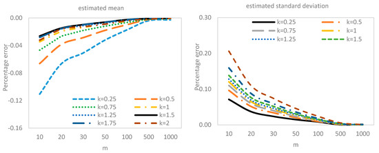
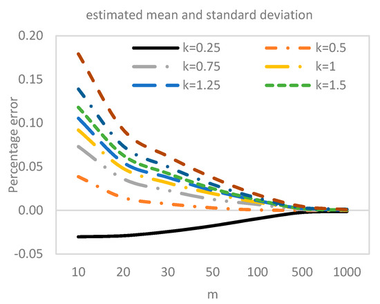
Figure 1. Control limits for the two-sided CUSUM chart when the in-control mean and standard deviation are either known or estimated $\left(n=5,{\mathrm{ARL}}_0=200\right)$.

4. The Outliers and CUSUM Chart with Estimated Parameters

The effect of estimation errors on the performance of a CUSUM chart may further be strained if there exist some extreme values in the Phase I samples. Both the in-control and the out-of-control ARL and SDRL values will be different from those of the theoretical CUSUM charts. In this section, we evaluated the effects of the outliers on the performance of a two-sided CUSUM control chart with estimated parameters. Using a simulation approach, outliers were generated from the mixture distribution, where $\left(1-\alpha \right)100\%$ regular observations were from $N(\widehat{\mu },{\widehat{\sigma }}^2)$ and the remaining $\alpha 100\%$ observations came from a multiple of ${\chi }_{\left(n\right)}^2$ with $n$ degrees of freedom, [28]. That is, each observation was generated from a mixture distribution

$$f\left(x\right)=\left(1-\alpha \right)N\left(\mu ,{\sigma }^2\right)+\alpha \left[N\left(\mu ,{\sigma }^2\right)+w{\chi }_{\left(1\right)}^2\right]$$

(10)

where $\alpha$ is the probability of having a multiple of ${\chi }_{\left(1\right)}^2$ added and $w\ge 1$ is the outlier model multiplier. A value of $\alpha =0$ indicates no presence of an outlier in the sampled data. Without loss of generality, we set $\mu =0$ and ${\sigma }^2=1$. The values of $w$ is set equal to 1, 2 or 3 corresponding to the small, medium and large outlier, respectively.

The mean and the variance of mixture distribution in Equation (10) are derived in Equations (11) and (12) respectively.

$$\begin{gathered} E\left(X\right)={\displaystyle \sum }_{p=1}^2{\omega }_p{\mu }_p \\ =\left(1-\alpha \right)E\left[N\left(\mu ,{\sigma }^2\right)\right]+\alpha E\left[N\left(\mu ,{\sigma }^2\right)+w{\chi }_{\left(1\right)}^2\right] \\ =\left(1-\alpha \right)\mu +\alpha \left(\mu +w\right) \\ =\mu +\alpha w \end{gathered}$$

(11)

$$\begin{gathered} Var\left(X\right)={\displaystyle \sum }_{p=1}^2{\omega }_p\left({\mu }_p^2+{\sigma }_p^2-{\left\{E\left(X\right)\right\}}^2\right) \\ =\left(1-\alpha \right)\left[{\left(E\left(N\left(\mu ,{\sigma }^2\right)\right)\right)}^2+V\left(N\left(\mu ,{\sigma }^2\right)\right)-{\left\{E\left(X\right)\right\}}^2\right] \\ + \alpha \left[{\left(E\left(N\left(\mu ,{\sigma }^2\right)+w{\chi }_{\left(1\right)}^2\right)\right)}^2+V\left(N\left(\mu ,{\sigma }^2\right)+w{\chi }_{\left(1\right)}^2\right)-{\left\{E\left(X\right)\right\}}^2\right] \\ =\left(1-\alpha \right)[{\mu }^2+{\sigma }^2-{\left\{\mu +\alpha w\right\}}^2]+\alpha [{\left\{\mu +w\right\}}^2+{\sigma }^2+2w^2-{\left\{\mu +\alpha w\right\}}^2] \\ =\left(1-\alpha \right)\left[{\mu }^2+{\sigma }^2-{\mu }^2-{\alpha }^2{w}^2-2\alpha w\mu \right]+\alpha \left[{\mu }^2+w^2+2w\mu +{\sigma }^2+2w^2-{\mu }^2-{\alpha }^2{w}^2-2\alpha w\mu \right] \\ =\left(1-\alpha \right)\left[{\sigma }^2-{\alpha }^2{w}^2-2\alpha w\mu \right]+\alpha \left[w^2+2w\mu +{\sigma }^2+2w^2-{\alpha }^2{w}^2-2\alpha w\mu \right] \\ ={\sigma }^2\left(1-\alpha +\alpha \right)-2\alpha w\mu \left(1-\alpha +\alpha \right)-{\alpha }^2{w}^2\left(1-\alpha +\alpha \right)+\alpha w^2+2\alpha w\mu +2\alpha w^2 \\ ={\sigma }^2-2\alpha w\mu -{\alpha }^2{w}^2+\alpha w^2+2\alpha w\mu +2\alpha w^2 \\ ={\sigma }^2+3\alpha w^2-{\alpha }^2{w}^2 \\ ={\sigma }^2+\alpha \left(3-\alpha \right)w^2 \end{gathered}$$

(12)

We set up a CUSUM chart using the same design parameters, $n,k,h$ and $m$ as in Section 3. he in-control ARL and SDRL values for the two-sided CUSUM chart based on this model with $\alpha =0.00,0.01,0.02,0.03$ and $0.04$ are presented in Table 7, Table 8 and Table 9. To save space, we restricted the study to in-control cases having seen the behavioral pattern for the out-of-control cases in Table 3, Table 4 and Table 5.

Table 7. In-control average run length (ARL) and standard deviation run length (SDRL) values for the two-sided CUSUM control chart in the presence of outlier when the in-control standard deviation is known, and mean is estimated $\left(n=5,{\mathrm{ARL}}_0=200\right)$.

m	k	h	RL Properties	w = 1					w = 2					w = 3
				α					α					α
				0.00	0.01	0.02	0.03	0.04	0.00	0.01	0.02	0.03	0.04	0.00	0.01	0.02	0.03	0.04
10	0.25	7.609	ARL	199	198	196	194	192	199	195	190	182	178	199	192	183	173	163
			SDRL	215	214	213	212	212	215	213	211	206	205	215	213	208	204	198
	0.50	4.447	ARL	200	199	198	196	195	200	195	191	187	180	200	194	185	177	167
			SDRL	211	210	211	210	209	211	209	206	206	200	211	210	204	201	196
	0.75	3.070	ARL	200	199	199	198	196	200	198	194	189	184	200	193	187	179	171
			SDRL	207	207	207	206	207	207	206	204	203	198	207	203	202	198	193
	1.00	2.290	ARL	200	199	198	197	196	200	197	195	189	186	200	195	189	182	176
			SDRL	205	203	204	202	202	205	202	202	198	196	205	201	199	195	191
50	0.25	7.071	ARL	200	198	197	194	192	200	197	190	181	169	200	192	179	164	147
			SDRL	191	189	190	187	186	191	189	184	177	169	191	187	177	166	154
	0.50	4.246	ARL	200	199	198	196	194	200	197	192	186	178	200	194	186	172	158
			SDRL	197	195	195	194	192	197	195	191	186	179	197	193	185	176	165
	0.75	2.968	ARL	200	199	199	198	195	200	198	195	189	184	200	196	188	179	167
			SDRL	198	197	198	197	195	198	198	195	190	185	198	195	189	182	172
	1.00	2.233	ARL	200	200	199	199	197	200	198	195	192	188	200	197	191	183	174
			SDRL	199	199	198	198	196	199	197	195	191	190	199	196	192	186	177
100	0.25	6.97	ARL	200	199	197	195	191	200	196	189	180	168	200	193	178	161	141
			SDRL	189	188	186	185	180	189	187	179	172	163	189	183	172	159	142
	0.50	4.212	ARL	200	200	200	196	195	200	198	193	187	177	200	196	185	173	156
			SDRL	196	196	196	192	192	196	193	189	185	176	196	192	183	173	158
	0.75	2.952	ARL	200	201	199	197	196	200	200	194	191	185	200	196	189	178	168
			SDRL	198	199	197	195	195	198	196	192	189	184	198	195	189	178	168
	1.00	2.224	ARL	201	199	201	199	197	201	199	196	194	188	201	199	192	185	173
			SDRL	199	198	200	197	197	199	197	195	193	188	199	198	192	185	174
500	0.25	6.878	ARL	200	199	197	195	189	200	196	189	177	164	200	194	179	156	134
			SDRL	188	187	187	183	178	188	184	177	166	154	188	181	168	146	126
	0.50	4.18	ARL	200	201	199	197	193	200	199	192	186	175	200	196	185	171	153
			SDRL	195	195	194	192	189	195	193	188	181	172	195	191	181	167	151
	0.75	2.938	ARL	200	201	199	197	195	200	200	195	190	183	200	198	191	180	166
			SDRL	198	198	196	195	193	198	197	193	187	180	198	195	190	179	164
	1.00	2.215	ARL	200	200	199	199	196	200	198	197	192	188	200	198	193	185	174
			SDRL	198	199	197	197	193	198	196	196	190	185	198	196	191	182	173
1000	0.25	6.870	ARL	200	201	198	193	190	200	198	190	178	163	200	194	178	156	134
			SDRL	188	189	186	181	179	188	186	178	166	153	188	182	167	144	124
	0.50	4.174	ARL	200	200	198	197	194	200	198	193	186	176	200	196	185	171	153
			SDRL	195	195	193	191	189	195	193	188	181	171	195	190	180	167	149
	0.75	2.936	ARL	200	199	199	197	196	200	200	197	191	183	200	198	191	179	166
			SDRL	198	195	197	194	194	198	198	194	189	180	198	195	189	175	165
	1.00	2.215	ARL	200	199	200	198	198	200	200	198	192	188	200	198	192	185	173
			SDRL	199	199	199	196	197	199	198	195	190	186	199	196	191	183	172

Table 8. In-control ARL and SDRL values for the two-sided CUSUM control chart in the presence of an outlier when the in-control mean is known, and the standard deviation is estimated $\left(n=5,{\mathrm{ARL}}_0=200\right)$.

m	k	h	RL Properties	w = 1					w = 2					w = 3
				α					α					α
				0.00	0.01	0.02	0.03	0.04	0.00	0.01	0.02	0.03	0.04	0.00	0.01	0.02	0.03	0.04
10	0.25	6.363	ARL	200	232	271	308	369	200	1252	2827	5180	7632	200	5766	13,029	22,028	33,346
			SDRL	308	720	1271	1442	2202	308	25,588	41,781	59,472	72,550	308	66,775	101,057	131,849	163,026
	0.50	3.769	ARL	200	253	320	402	498	200	2374	5025	8677	13,606	200	8574	19,938	32,755	49,639
			SDRL	374	1216	1839	2660	3384	374	39,571	59,416	79,131	100,612	374	82,482	127,093	162,747	200,013
	0.75	2.610	ARL	201	266	374	471	569	201	2614	6115	10,306	15,478	201	10,440	23,698	39,039	56,370
			SDRL	405	1397	2665	3349	3891	405	41,686	66,631	86,598	107,915	405	92,015	139,038	178,484	213,382
	1.00	1.947	ARL	200	289	386	484	599	200	3152	6751	10,527	16,605	200	10,322	24,092	40,720	59,187
			SDRL	420	1851	2745	3539	4090	420	46,733	69,185	87,750	111,809	420	91,131	140,118	181,993	218,900
50	0.25	6.750	ARL	200	213	229	245	262	200	249	313	399	522	200	320	598	1020	2048
			SDRL	209	225	249	271	298	209	304	455	892	1381	209	958	6844	9008	19,563
	0.50	4.087	ARL	201	220	240	263	287	201	274	377	550	767	201	413	1043	2332	5481
			SDRL	230	259	294	328	379	230	453	1093	4144	4185	230	2854	11,610	24,597	45,072
	0.75	2.863	ARL	201	221	245	272	299	201	288	425	614	970	201	499	1284	3489	7734
			SDRL	241	274	314	379	417	241	655	1509	2443	7384	241	5406	14,261	32,417	56,026
	1.00	2.155	ARL	200	223	248	275	309	200	295	453	713	1113	200	517	1622	3965	9219
			SDRL	246	285	340	383	450	246	628	3646	5086	8738	246	5297	19,603	35,460	63,990
100	0.25	6.794	ARL	199	212	226	242	257	199	240	294	360	440	199	284	416	621	984
			SDRL	197	210	229	246	266	197	250	329	427	573	197	334	636	1439	2903
	0.50	4.131	ARL	201	218	237	258	281	201	258	335	437	582	201	333	555	1005	1883
			SDRL	213	235	258	284	315	213	301	428	616	953	213	1159	1079	5010	9240
	0.75	2.898	ARL	200	221	243	265	292	200	267	358	494	671	200	351	649	1290	2600
			SDRL	219	244	276	302	338	219	330	495	799	1297	219	586	2578	7319	14,579
	1.00	2.183	ARL	200	221	242	270	295	200	269	376	517	718	200	360	700	1417	3124
			SDRL	221	249	277	321	349	221	340	555	948	1354	221	595	2335	6141	18,020
500	0.25	6.848	ARL	201	213	227	242	257	201	238	284	340	411	201	272	375	523	735
			SDRL	191	203	218	232	248	191	228	278	337	412	191	267	381	550	807
	0.50	4.165	ARL	200	218	237	255	276	200	251	317	399	510	200	298	454	702	1098
			SDRL	199	216	236	256	280	199	253	326	416	543	199	306	492	796	1317
	0.75	2.928	ARL	201	218	240	261	286	201	257	333	435	565	201	315	499	814	1350
			SDRL	202	221	243	265	292	202	264	347	463	613	202	330	554	963	1698
	1.00	2.209	ARL	200	219	241	264	291	200	261	343	455	597	200	321	527	882	1509
			SDRL	203	222	247	272	298	203	269	361	488	652	203	341	595	1052	1921
1000	0.25	6.851	ARL	200	214	227	240	256	200	237	284	339	405	200	269	368	514	717
			SDRL	189	203	216	228	244	189	227	273	330	401	189	260	362	517	740
	0.50	4.171	ARL	201	219	235	254	277	201	251	313	396	501	201	295	445	681	1058
			SDRL	197	216	233	251	277	197	249	314	402	512	197	298	457	726	1138
	0.75	2.933	ARL	201	220	240	262	285	201	258	332	432	558	201	311	490	784	1280
			SDRL	200	220	240	263	288	200	259	338	442	578	200	318	516	840	1420
	1.00	2.210	ARL	200	219	242	265	289	200	261	340	446	586	200	317	511	844	1408
			SDRL	200	221	244	267	290	200	264	349	460	612	200	329	542	911	1580

Table 9. In-control ARL and SDRL values for the two-sided CUSUM control chart in the presence of an outlier when the in-control mean and standard deviation are estimated $\left(n=5,{\mathrm{ARL}}_0=200\right)$.

m	k	h	RL Properties	w = 1					w = 2					w = 3
				α					α					α
				0.00	0.01	0.02	0.03	0.04	0.00	0.01	0.02	0.03	0.04	0.00	0.01	0.02	0.03	0.04
10	0.25	7.059	ARL	200	220	238	257	264	200	289	420	506	522	200	415	667	834	1018
			SDRL	344	579	802	1325	880	344	2389	8400	8836	7702	344	6970	12,597	13,937	15,538
	0.50	4.010	ARL	201	244	315	333	390	201	691	1221	2017	2556	201	2465	4835	7722	10,719
			SDRL	404	1375	5270	4092	5614	404	15,507	21,367	30,537	34,157	404	38,100	54,564	70,640	84,741
	0.75	2.719	ARL	199	291	340	409	497	199	1402	2839	4258	6234	199	4856	10,452	18,230	25,507
			SDRL	429	5091	5290	5868	8207	429	27,821	40,327	50,689	62,254	429	58,258	87,142	116,950	139,084
	1.00	2.010	ARL	200	280	396	468	642	200	1919	3740	6103	8942	200	7038	15,601	24,673	35,470
			SDRL	444	2471	7494	7088	11,812	444	33,960	48,185	62,320	77,490	444	72,692	109,882	138,233	165,823
50	0.25	6.917	ARL	201	212	227	233	242	201	238	268	297	319	201	265	323	366	391
			SDRL	212	228	250	259	270	212	276	331	381	429	212	355	474	560	616
	0.50	4.169	ARL	201	218	236	253	271	201	260	326	405	482	201	333	495	715	977
			SDRL	231	259	290	312	345	231	371	528	684	894	231	678	1371	2239	3977
	0.75	2.913	ARL	200	222	242	265	289	200	276	372	497	642	200	393	719	1281	2057
			SDRL	240	282	313	352	392	240	454	738	1374	1769	240	1885	4811	9559	14,183
	1.00	2.193	ARL	199	221	247	273	297	199	282	402	554	770	199	435	925	1826	3613
			SDRL	244	281	333	382	419	244	488	928	1704	3350	244	1775	7761	14,799	28,661
100	0.25	6.917	ARL	200	211	223	232	241	200	234	266	291	310	200	262	313	350	368
			SDRL	198	210	225	237	248	198	242	285	318	345	198	287	356	409	440
	0.50	4.169	ARL	200	217	234	252	268	200	252	311	375	441	200	302	434	591	767
			SDRL	213	231	256	277	299	213	285	378	470	570	213	388	606	906	1233
	0.75	2.913	ARL	200	219	238	261	280	200	260	337	430	546	200	330	526	816	1212
			SDRL	218	243	266	298	325	218	311	434	584	811	218	472	895	1682	2721
	1.00	2.193	ARL	200	222	242	268	290	200	269	358	474	619	200	347	596	1016	1662
			SDRL	222	252	278	311	339	222	336	489	703	994	222	586	1330	2710	4963
500	0.25	6.868	ARL	200	210	222	232	240	200	233	263	286	302	200	260	311	340	352
			SDRL	190	201	212	222	231	190	224	255	280	295	190	253	306	341	352
	0.50	4.171	ARL	200	215	232	248	264	200	247	302	359	414	200	288	402	528	662
			SDRL	199	216	231	247	265	199	248	307	369	429	199	297	420	561	712
	0.75	2.93	ARL	200	218	237	258	277	200	256	323	403	496	200	307	459	670	947
			SDRL	201	220	240	264	281	201	262	336	424	530	201	320	499	747	1071
	1.00	2.209	ARL	200	219	240	262	285	200	260	335	430	545	200	317	495	762	1164
			SDRL	203	224	244	269	296	203	269	350	456	590	203	335	545	865	1382
1000	0.25	6.860	ARL	200	212	223	232	239	200	234	264	287	302	200	258	310	339	346
			SDRL	189	200	211	222	228	189	224	254	275	293	189	248	302	329	336
	0.50	4.172	ARL	200	215	232	248	263	200	247	300	357	416	200	289	399	523	653
			SDRL	197	213	230	245	261	197	244	301	359	418	197	289	406	534	675
	0.75	2.933	ARL	200	218	238	257	277	200	256	322	398	491	200	304	453	659	927
			SDRL	200	219	239	258	278	200	257	326	409	507	200	309	466	690	986
	1.00	2.213	ARL	200	218	240	262	285	200	259	333	425	542	200	313	489	752	1124
			SDRL	201	218	240	265	289	201	264	338	436	562	201	320	511	801	1219

From Table 7, Table 8 and Table 9, it was observed that estimating $\mu$, $\sigma$ or both in the presence of outliers, $\alpha >0$ to set up a CUSUM chart had a significant effect on the ARL and SDRL performance of the chart. Particularly, when the number of Phase I samples, $m$ was small. The in-control ARLs were approximately equal to the limiting value of 200 when $\alpha =0$. As expected, the RL values were directly proportional to $k$ and $\alpha$. That is, the in-control ARL and SDRL deteriorated with the increasing number of the false alarm rate as $k$, $\alpha$ or both the design parameters increased. In fact, the deterioration level became more alarming with the increase in an outlier metric multiplier, $w>1$. Furthermore, as the number of Phase I samples increased, the ARL approached its theoretical value and much faster than its corresponding SDRL (cf. Table 7). However, this was not the case for Table 8 and Table 9, when $m\ge 500$. In general, increasing the number of Phase I data will reduce the occurrence of false alarm and bring the RL to be closer to the theoretical value. Unfortunately, this may not be visible in practice. Thus, we suggest a design structure based on the robust Tukey outlier detection model.

5. Performance of the Tukey CUSUM Control Chart

In this section, we studied the performance of the proposed Tukey model based CUSUM control chart with estimated parameters. Let $X_1,X_2,\dots ,X_n$ denote Phase I samples and $\check{X}$ be the median samples. Then an observation $X_k$ from $X_1,X_2,\dots ,X_n$ is declared as an outlier if $\left|X_k-\check{X}\right|>p\times IQR$, where $IQR=Q_3-Q_1$ is the interquartile range. $Q_1$ and $Q_3$ are the first and third quartile of $X_1,X_2,\dots ,X_n$, corresponding to the 25th and 75th percentile, respectively. The constant, $p$ is the confidence factor commonly chosen between 1.5 and 3.0. The confidence factor of Tukey’s detector is selected so that it is not too small leading to unnecessary screening of observations that are not outliers, and at the same time it should not be too large implying the inability of the detector to detect any outliers. For the said reason, $p$ is chosen to be $2.2$ for the current study (for more details on the Tukey’s outlier detector see, Tukey [28]).

Once an outlier is detected from the Phase I sample using Tukey’s model, it is screened and the remaining data points are used to estimate mean and variance of the process. After screening the suspected outliers, distribution of the remaining data points in Phase I is revised from a mixture distribution to a truncated mixture distribution. Here, the truncation limits are set to be $LDL=\check{X}-2.2\times IQR$ and $UDL=\check{X}+2.2\times IQR$ where $LDL$ and $UDL$ are lower and upper detection limits, respectively. Finally, the truncated mean and variance for the Phase I data points are defined, respectively, as follows:

$$E\left(X | LDL<X<UDL\right)=\frac{{{\displaystyle \int }}_{LDL}^{UDL}xg\left(x\right)dx}{F_X\left(UDL\right)-F_x\left(LDL\right)}$$

(13)

$$Var\left(X | LDL<X<UDL\right)=\frac{{{\displaystyle \int }}_{LDL}^{UDL}{x}^{2}g\left(x\right)dx}{F_X\left(UDL\right)-F_x\left(LDL\right)}-{\left[E\left(X | LDL<X<UDL\right)\right]}^2$$

(14)

where $g\left(x\right)=\{\begin{array}{l}f\left(x\right) \forall LDL<x<UDL\hfill \\ 0 \mathrm{otherwise}\hfill \end{array}$ and $F_X(.)$. is the cumulative distribution function of $X$. The truncated mean and variance in Equations (13) and (14) are evaluated for different values of $\alpha$ and $w$, and are given in Table 10.

Table 10. Non-truncated and truncated mean and variance of mixture distribution of $N\left(0,1\right)$ and ${\chi }_{\left(1\right)}^2$.

$\mathit{\alpha }$		$\mathit{w}$
		1		2		3
		$\mathit{X}$	$\mathit{X} | \mathit{L}\mathit{D}\mathit{L}<\mathit{X}<\mathit{U}\mathit{D}\mathit{L}$	$\mathit{X}$	$\mathit{X} | \mathit{L}\mathit{D}\mathit{L}<\mathit{X}<\mathit{U}\mathit{D}\mathit{L}$	$\mathit{X}$	$\mathit{X} | \mathit{L}\mathit{D}\mathit{L}<\mathit{X}<\mathit{U}\mathit{D}\mathit{L}$
0	$E(.)$	0	−0.00007	0	0.0001	0	0.00006
	$V(.)$	1	0.97097	1	0.97101	1	0.971
0.01	$E(.)$	0.01	0.0051	0.02	0.00564	0.03	0.00539
	$V(.)$	1.0299	0.97727	1.1196	0.97881	1.2691	0.97878
0.02	$E(.)$	0.02	0.01064	0.04	0.01127	0.06	0.01083
	$V(.)$	1.0596	0.98373	1.2384	0.9866	1.5364	0.98683
0.03	$E(.)$	0.03	0.01624	0.06	0.01713	0.09	0.01664
	$V(.)$	1.0891	0.99016	1.3564	0.99458	1.8019	0.99498
0.04	$E(.)$	0.04	0.02158	0.08	0.02323	0.12	0.0223
	$V(.)$	1.1184	0.99666	1.4736	1.00311	2.0656	1.00392
0.05	$E(.)$	0.05	0.027	0.1	0.02928	0.15	0.0284
	$V(.)$	1.1475	1.00323	1.59	1.01156	2.3275	1.01339
0.06	$E(.)$	0.06	0.03274	0.12	0.03568	0.18	0.03429
	$V(.)$	1.1764	1.00988	1.7056	1.02088	2.5876	1.02238
0.07	$E(.)$	0.07	0.03847	0.14	0.04203	0.21	0.04068
	$V(.)$	1.2051	1.01709	1.8204	1.02994	2.8459	1.03251
0.08	$E(.)$	0.08	0.04424	0.16	0.04859	0.24	0.04752
	$V(.)$	1.2336	1.02381	1.9344	1.03942	3.1024	1.04268
0.09	$E(.)$	0.09	0.05017	0.18	0.05536	0.27	0.0539
	$V(.)$	1.2619	1.03107	2.0476	1.04928	3.3571	1.05381
0.1	$E(.)$	0.1	0.05596	0.2	0.06209	0.3	0.06083
	$V(.)$	1.29	1.03811	2.16	1.05968	3.61	1.06487

Table 10 clearly indicates that mixing $\alpha \left(100\right)\%$ outliers in the distribution disturbs the mean and variance, especially for the larger values of $w$. On contrary, when the distribution is truncated (i.e., Tukey’s outlier detector is applied) this disturbance in the mean and variance is negligible. In view of this discussion, the estimates of the process mean, and variance obtained from the truncated distribution (i.e., after screening the data using Tukey’s model) will have the minimal effect of outliers introduced in the Phase I samples.

Using the same design structure and parameters as in Section 3 and Section 4, we computed the in-control ARL and SDRL values for the two-sided CUSUM control chart based on the Tukey outlier detection model with the estimated parameters. Three cases were considered, when the mean, the standard deviation or both were estimated. To access the performance of the proposed charts, we present in Figure 2, Figure 3 and Figure 4, a graphical display of the in-control ARL values with $m=10,100,500$ and $1000$ when the magnitude of outlier multiplier $w$ is small ($w=1$), medium ($w=2$) and large ($w=3$). We presented only the case when both the mean and the standard deviation were estimated, as the other two cases had similar conclusions. Furthermore, we also showed the in-control ARL values in the presence of outliers without screening in Figure 2, Figure 3 and Figure 4 for a quick comparison. With the two charts side-by-side, we outlined our findings under the following headings.

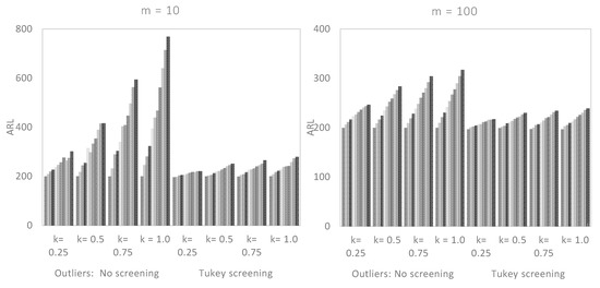
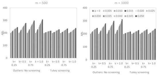
Figure 2. In-control ARL values for the two-sided CUSUM control chart in the presence of an outlier, with and without screening, when the parameters are estimated $\left(w=1,n=5,{\mathrm{ARL}}_0=200\right)$.

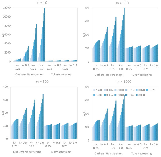
Figure 3. In-control ARL values for the two-sided CUSUM control chart in the presence of an outlier, with and without screening, when the parameters are estimated $\left(\mathrm{w}=2,\mathrm{n}=5,{\mathrm{ARL}}_0=200\right)$.

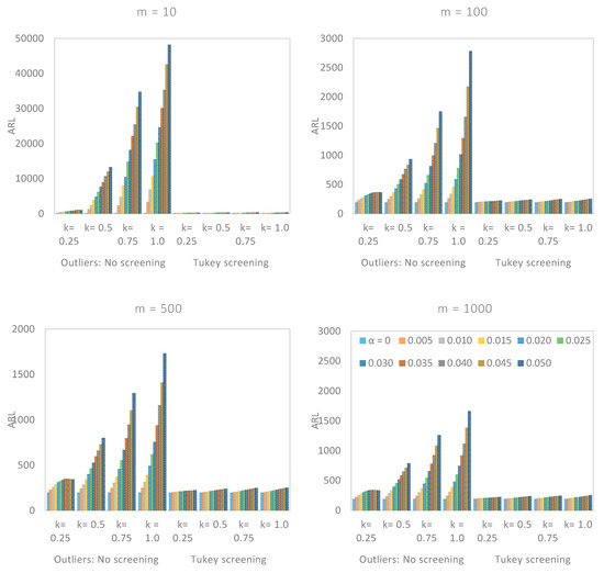
Figure 4. In-control ARL values for the two-sided CUSUM control chart in the presence of an outlier, with and without screening, when the parameters are estimated $\left(w=3,n=5,{\mathrm{ARL}}_0=200\right)$.

5.1. Performance Comparison with Respect to m

We saw earlier that the number of Phase I data, $m$， did have a significant effect on the performance of a CUSUM chart. From Figure 2, Figure 3 and Figure 4, we saw that there was a vast difference in the reported ${\mathrm{ARL}}_0$ between non-screened data and when the robust Tukey outlier detection model was applied to construct a CUSUM chart, particularly when $m$ was small. For example, in Figure 3, if $m=10,k=1.0$ and $\alpha >0.04$, the ${\mathrm{ARL}}_0$ for non-screened data were in five figures while the corresponding Tukey screened data were relatively closed to the target value. Even an increase in the number of Phase I observations with no screening did not appear to have a significant impact on the chart’s performance as the outlier multiplier increased. The Tukey screened counterpart, however, was getting closer to the limiting value ${\mathrm{ARL}}_0=200$, as $m$ increased.

In other words, the use of the Tukey outlier detector in the construction of a CUSUM chart would maintain the performance of the chart, even with the handful amount of Phase I data.

5.2. Performance Comparison with Respect to α

If $\alpha =0$, the in-control ARL values of CUSUM charts were approximately equal to the theoretical value of $200$ and indicates the absence of outliers in the Phase I sampled data. However, as the magnitude of $\alpha$ increased, the non-screened data blew out of proportion, particularly when $m$ was small and $k>0.5$. For example, if $m=10,k=1.0$ and $\alpha =0.05$, in Figure 2, the ${\mathrm{ARL}}_0$ for the non-screened observations was 770 as against to 280 when the Tukey outlier detection model was applied. Even with the large values of $k$ and $\alpha$, the Tukey screened data appeared to be getting closer to the nominal value as $m$ increased. The same conclusion could not be made for non-screened data, as the in-control ARL values remained high when $\alpha$ was relatively large (cf. Figure 2, Figure 3 and Figure 4). This means that the Tukey’s model would not only keep the ${\mathrm{ARL}}_0$ on target but also maintain the performance of the CUSUM control chart. In general, we observed that the effect of $\alpha$ was minimal when $k$ was small.

5.3. Performance Comparison with Respect to w

The larger the magnitude of outlier multiplier $w$, the worst the in-control ARL value of a two-sided CUSUM chart. If the outliers in a Phase I data were not screened, the ${\mathrm{ARL}}_0$ was so huge as $w$ increased, that the capability of the CUSUM chart in process monitoring was seriously affected. Unlike the Tukey based chart that tried to maintain the ${\mathrm{ARL}}_0$ at the target value. For example, if $m=10,k=0.25$ and $\alpha =0.05$, the in-control ARL values for the non-screened data were $302,634$ and 1025 when $w=1,2$ and $3$, respectively. Compared to the screened Phase I data by the Tukey’s model with ARL values of 217, 222 and 225. Thus, the Tukey CUSUM chart could relatively withstand the impact of outlier multiplier $w$ as compared to the chart based on non-screened data.

6. Illustrative Example

For illustrating the application of Tukey’s outlier detectors with the CUSUM control chart, we used a dataset from [3]. The variable of interest was the flow width measurement (in microns) for the hard-brake process. The data consisted of twenty-five in-control Phase I samples and twenty out-of-control Phase II samples where the average width had increased due to an assignable cause(s). The process mean and standard deviation were estimated (cf. Equations (2)–(4)) from Phase I samples and were found to be $1.5056$ and $0.14$, respectively. These estimates were used to set up a CUSUM control chart for Phase II samples.

It is clearly observed from the scatter plot given in Figure 5a that the observations were relocated in Phase II. Further, it might also be confirmed from the CUSUM chart plotted in Figure 5b, which indicates several out-of-control signals in Phase-II. These findings led to the evidence that the hard-brake process had a positive shift at subgroup number fifteen and onwards.

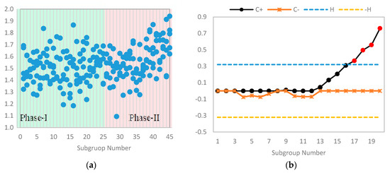
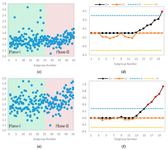
Figure 5. Scatter plots and the CUSUM control chart outputs for the dataset on the width of the hard-brake process.

Now using the data perturbation technique (cf. Kargupta, Datta [29] and Liu, Kargupta [30]), we introduced random outliers in different subgroups. Further, the process mean and standard deviation were estimated and found out to be $1.554$ and $0.21544$, respectively. Based on these estimates, we constructed the limits, which were further used to monitor the location of Phase II samples. In Figure 5c, the scatter plot depicts a slight upward change in Phase II, and control chart presented in Figure 5d shows that the out-of-control situation in Phase II was delayed (to subgroup number twenty) due to a small number of outliers present in Phase I. This happened because the limits widened due to the variation in Phase I estimates of process mean and standard deviation.

Finally, by using the above-mentioned contaminated Phase I data, we estimated the limit of the Tukey’s outlier detector, which was found to be $p\times IQR=0.44726$. Now for any value, the absolute deviation from the median (i.e., $\left|X-1.5171\right|$) greater than $0.44726$ implies that the corresponding value is an outlier and needs to be screened from the data. Hence, by using the outlier detector, six observations were screened from the Phase I data. Further, the process mean and standard deviation were estimated and found out to be $1.5123$ and $0.152$, respectively. These new estimates were similar to the estimates of the original data and the scatter plot of the data is given in Figure 5e, which also showed upward trend in Phase II. In Figure 5f, the control chart is presented, which revealed that the there was no change in the limits, but the chart had detected an increase in the process mean at subgroup number sixteen.

7. Practical Application

In recent years, activity recognition (AR) became an emerging research topic due to the advancement of electronic devices. AR is commonly used in pattern recognition, ubiquitous computing, human behavior modeling and human–machine interaction. In health care studies, different electronic devices are commonly used to recognize everyday life activities. In eldercare centers, these facilities provide assistance and care to the elders and help to ensure their safety and successful aging. Commonly, wearable devices and cameras are used to monitor everyday life activities, but these approaches suffer from several disadvantages such as intrusiveness, time-consuming processing and low resolution. Therefore, to overcome these challenges in real-time activity recognition, Hong, Kang [31] used an alternative method named as multisensor data fusion (assembly reliability evaluation method—AReM). For a more detailed introduction on the AReM see [32]. In the AReM system, information is gathered from an inertial sensor embedded in a smartphone and wireless sensor system, which is plugged between the user and environment. Further, in a wireless sensor network, the movement of an individual is measured in the received signal strength (RSS) between the user and environment. For the AR dataset [31], designed a competition. In which three IRIS motes are used and placed on the chest, the right and left ankle of an actor (cf. Figure 6).

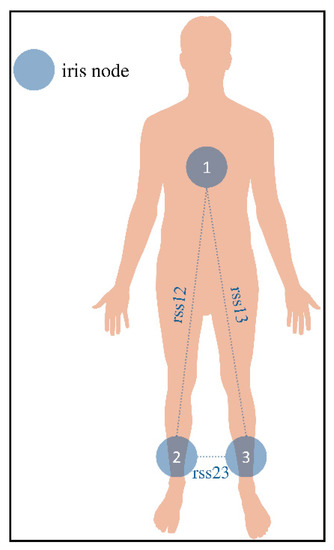
Figure 6. Placement of IRIS nodes on the actor’s body (cf. (Palumbo, Gallicchio [33]).

From this wireless sensor network, data was recorded on the actor’s activities such as; bending, cycling, standing, sitting, laying and walking. Further, for the first task of heterogeneous AReM, they considered activities such as cycling and standing. For the application purpose, we were concerned to detect a change in the pattern of RSS generated through the heterogeneous AReM setup. The AR time series dataset contained 480 observations in total, and each observation was obtained after 250 milliseconds. The average of RSS against the three IRIS motes (i.e., rss12, rss13, and rss23) was available in 15 different sequences of each activity. In our application, we considered the first sequence of the rss13 IRIS mote (chest-left ankle). The average of RSS of cycling was considered as in-control Phase I samples and average RSS of standing was considered as the out-of-control Phase II sample points. To access the normality of Phase I data set, we plotted a probability plot at the 95% confidence interval (cf. Figure 7) and also applied the Anderson–Darling test ($\mathrm{AD}=0.517$ and $p-\mathrm{value}=0.189$), which provided the evidence that the Phase I data set was normal.

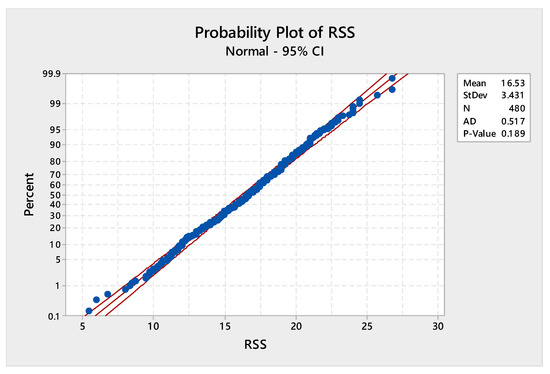
Figure 7. Probability plot of the received signal strength (RSS) values of the rss13 mote belonging to the cycling activity.

The RSS values of the chest-left ankle mote belonging to the cycling activity were clubbed into Phase I subgroups, and only the first 50 subgroups were used for the plotting purpose. Moreover, the first 25 subgroups based on the RSS values of chest-left ankle mote belonging to the standing activity were used as Phase II samples. The dataset of 75 subgroups is reported in Table 11. The process mean and standard deviation were estimated from the Phase I samples and found to be 16.9734 and 3.4764, respectively. These estimates were then used to construct the CUSUM chart for the Phase II samples. Figure 8a,b presents the scatter plot for the original data and the control chart output, respectively.

Table 11. Phase-I subgroups of RSS values chest-left ankle mote. Phase-II subgroups of RSS values chest-left ankle mote.

Phase-I Subgroups of RSS Values Chest-Left Ankle Mote
No	RSS											${\overline{\mathbf{X}}}_{\mathbf{i}}$		${\mathbf{S}}_{\mathbf{i}}$
1	17.50	21.50			17.75		20.50			14.25		18.300		2.847
2	11.80	21.50			23.33		18.50			18.00		18.626		4.399
3	18.00	17.50			15.33		16.25			18.75		17.166		1.372
4	12.50	17.50			16.00		19.25			13.00		15.650		2.892
5	22.00	20.25			16.25		15.33			17.75		18.316		2.776
6	16.50	24.00			22.75		20.75			20.75		20.950		2.847
7	24.50	13.25			18.25		23.00			19.00		19.600		4.418
8	13.00	15.33			17.33		12.33			22.50		16.098		4.089
9	20.50	14.50			16.75		17.25			13.33		16.466		2.769
10	17.50	17.25			13.75		17.67			14.67		16.168		1.823
11	14.00	13.00			19.00		16.00			11.25		14.650		2.977
12	18.00	17.00			17.50		24.00			16.00		18.500		3.162
13	14.75	12.50			17.75		10.67			20.25		15.184		3.874
14	18.00	11.75			12.00		19.75			12.75		14.850		3.744
15	18.00	16.67			17.67		12.80			19.25		16.878		2.459
16	19.75	24.00			15.67		21.33			19.67		20.084		3.027
17	26.75	17.75			22.75		16.00			11.75		19.000		5.858
18	11.25	19.67			23.75		15.75			17.00		17.484		4.641
19	19.25	16.50			15.25		19.25			16.25		17.300		1.841
20	6.00	13.50			15.00		10.25			18.00		12.550		4.604
21	11.33	13.00			16.50		19.50			19.25		15.916		3.669
22	10.00	13.00			19.50		19.00			18.50		16.000		4.257
23	12.25	19.00			14.50		15.00			18.00		15.750		2.739
24	19.75	16.00			12.50		16.75			17.50		16.500		2.640
25	15.75	17.75			19.00		19.00			10.33		16.366		3.626
26	19.00	24.00			25.75		17.33			19.75		21.166		3.552
27	19.25	22.50			16.75		11.50			18.75		17.750		4.058
28	10.67	16.50			17.33		16.33			13.25		14.816		2.788
29	19.00	20.75			13.50		18.25			16.50		17.600		2.753
30	5.50	17.50			16.00		9.75			11.50		12.050		4.843
31	20.67	8.50			14.25		14.00			18.75		15.234		4.737
32	18.75	16.25			14.00		21.00			22.33		18.466		3.402
33	13.50	17.50			18.33		17.00			15.75		16.416		1.879
34	20.50	16.75			17.00		21.00			19.50		18.950		1.972
35	18.33	15.75			15.00		20.75			15.67		17.100		2.404
36	16.00	20.25			24.50		15.00			16.67		18.484		3.902
37	18.75	19.75			12.33		15.25			21.67		17.550		3.735
38	22.25	13.75			20.75		21.00			16.75		18.900		3.543
39	18.75	16.67			13.75		12.00			18.50		15.934		2.971
40	12.25	14.75			11.00		17.25			8.33		12.716		3.431
41	21.25	20.25			14.00		17.50			17.33		18.066		2.842
42	21.75	15.75			15.00		19.25			16.33		17.616		2.817
43	19.75	16.67			17.00		16.50			15.00		16.984		1.726
44	18.67	21.33			18.25		16.67			17.75		18.534		1.732
45	15.00	16.33			19.00		17.00			17.50		16.966		1.474
46	14.00	19.00			17.75		26.75			15.00		18.500		5.034
47	17.25	20.50			18.50		19.00			20.00		19.050		1.280
48	18.00	10.50			11.67		16.67			18.00		14.968		3.610
49	8.75	20.75			21.00		8.00			21.00		15.900		6.875
50	16.00	12.00			18.25		12.00			14.75		14.600		2.684
Phase-II Subgroups of RSS Values Chest-Left Ankle Mote.
No	RSS							${\overline{X}}_i$	$CUSU{M}_i^{+}$		$CUSU{M}_i^{-}$		$H$		$-H$
1	11.50	13.50	12.00	11.50		12.00		12.100	0.000		−4.096		6.41		−6.41
2	11.00	12.00	16.00	11.67		17.60		13.654	0.000		−6.638		6.41		−6.41
3	12.75	15.50	6.50	10.33		18.00		12.616	0.000		−10.218		6.41		−6.41
4	9.50	2.00	11.60	12.00		12.00		9.420	0.000		−16.994		6.41		−6.41
5	12.00	6.00	12.50	12.50		13.33		11.266	0.000		−21.924		6.41		−6.41
6	12.00	13.25	11.25	12.00		13.25		12.350	0.000		−25.770		6.41		−6.41
7	16.33	11.75	18.00	9.75		15.00		14.166	0.000		−27.800		6.41		−6.41
8	4.50	16.75	13.67	8.25		15.00		11.634	0.000		−32.362		6.41		−6.41
9	12.25	4.00	11.75	6.50		12.00		9.300	0.000		−39.258		6.41		−6.41
10	8.50	11.00	9.50	12.25		11.75		10.600	0.000		−44.854		6.41		−6.41
11	12.00	12.25	11.00	12.00		13.25		12.100	0.000		−48.950		6.41		−6.41
12	18.25	12.00	17.00	11.00		12.25		14.100	0.000		−51.046		6.41		−6.41
13	15.50	14.00	14.00	9.00		8.75		12.250	0.000		−54.992		6.41		−6.41
14	15.00	14.00	13.00	11.25		10.00		12.650	0.000		−58.538		6.41		−6.41
15	4.33	12.50	14.00	12.00		8.00		10.166	0.000		−64.568		6.41		−6.41
16	12.75	12.00	10.75	12.00		12.00		11.900	0.000		−68.864		6.41		−6.41
17	18.75	9.75	13.00	12.00		16.50		14.000	0.000		−71.060		6.41		−6.41
18	16.50	12.50	12.25	14.75		10.50		13.300	0.000		−73.956		6.41		−6.41
19	13.75	13.67	12.00	5.00		3.50		9.584	0.000		−80.568		6.41		−6.41
20	11.00	12.00	13.00	10.75		8.00		10.950	0.000		−85.814		6.41		−6.41
21	13.25	12.00	11.00	12.00		11.00		11.850	0.000		−90.160		6.41		−6.41
22	18.00	11.00	11.67	16.00		16.25		14.584	0.000		−91.772		6.41		−6.41
23	13.75	11.00	4.67	17.50		11.50		11.684	0.000		−96.284		6.41		−6.41
24	6.67	11.67	12.75	11.33		7.67		10.018	0.000		−102.462		6.41		−6.41
25	11.50	12.33	6.67	10.00		2.67		8.634	0.000		−110.024		6.41		−6.41

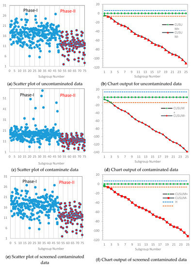
Figure 8. Scatter plots and CUSUM control chart outputs for the dataset on the received signal strength process.

It was evident from Figure 8a that there was a downward relocation in Phase II samples, a point equally supported by the corresponding CUSUM chart, which gave an out-of-control signal right from the start of the plots in Figure 8b. Now to access the effect of the outliers, we followed the same procedure as described in Section 6, by first contaminating the Phase I data and used the estimates obtained, ${\widehat{\mu }}_0=18.9924$ and ${\widehat{\sigma }}_0=7.4018$ to setup a CUSUM control chart for the Phase II data (cf. Figure 8c,d). Secondly, we used the Tukey outlier detector to screen the Phase I samples, computed the control chart parameters and used the estimates, ${\widehat{\mu }}_0=17.0593$ and ${\widehat{\sigma }}_0=3.5543$ to construct the CUSUM chart for the Phase II samples (cf. Figure 8e,f).

The introduction of outliers in the Phase I samples, Figure 8c gave rise to wider control limits, which in turn delayed the out-of-control signal in the Phase II control chart setup (cf. Figure 8d). However, the application of the outlier detector on the contaminated Phase I data resulted in the screening out of about ten data points (cf. Figure 8e). Subsequently, the corresponding CUSUM chart in Figure 8f shows a similar behavioral pattern as those of the original data in Figure 8b.

8. Conclusions

In this article, we evaluated the in-control performance of a two-sided CUSUM control chart when the parameters were estimated in the presence of outliers based on the robust Tukey detection model. Using a Monte Carlo simulation approach, the ARL and SDRL were computed for a different number of Phase I data.

The results show that a large number of Phase I data was required to minimize the practitioner-to-practitioner variability. In the presence of outliers, a larger amount of Phase I data was needed, which might not be realistic in practical applications. The results further revealed that the use of the Tukey outlier detector in the construction of a two-sided CUSUM control chart required fewer Phase I observations to stabilize the chart’s performance. Therefore, it was plausible to use the Tukey’s model in the design structure of a CUSUM chart when the parameters were estimated for efficient process monitoring, particularly when the observations were prone to outliers. The advantage of this proposal is its simplicity to design and it is easy to use. A point demonstrated by the illustrative and application examples of the new Tukey CUSUM control chart. The scope of this study might be extended to other control charts design strategies like the Shewhart and exponentially weighted moving average.

References

- Abujiya, M.a.R.; Riaz, M.; Lee, M.H. Enhanced cumulative sum charts for monitoring process dispersion. PLoS ONE 2015, 10, e0124520. [Google Scholar] [CrossRef] [PubMed]
- Page, E.S. Continuous inspection schemes. Biometrika 1954, 41, 100–114. [Google Scholar] [CrossRef]
- Montgomery, D.C. Introduction to Statistical Quality Control, 6th ed.; John Wiley & Sons: New York, NY, USA, 2009. [Google Scholar]
- Saleh, N.A.; Zwetsloot, I.M.; Mahmoud, M.A.; Woodall, W.H. CUSUM charts with controlled conditional performance under estimated parameters. Qual. Eng. 2016, 28, 402–415. [Google Scholar] [CrossRef]
- Schoonhoven, M.; Nazir, H.Z.; Riaz, M.; Does, R.J. Robust location estimators for the X-bar control chart. J. Qual. Technol. 2011, 48, 363–379. [Google Scholar] [CrossRef]
- Nazir, H.Z.; Riaz, M.; Does, R.J.M.M.; Abbas, N. Robust CUSUM control charting. Qual. Eng. 2013, 25, 211–224. [Google Scholar] [CrossRef]
- Amdouni, A.; Castagliola, P.; Taleb, H.; Celano, G. A variable sampling interval Shewhart control chart for monitoring the coefficient of variation in short production runs. Int. J. Prod. Res. 2017, 55, 5521–5536. [Google Scholar] [CrossRef]
- Abid, M.; Nazir, H.Z.; Riaz, M.; Lin, Z. Investigating the Impact of Ranked Set Sampling in Nonparametric CUSUM Control Charts. Qual. Reliab. Eng. Int. 2017, 33, 203–214. [Google Scholar] [CrossRef]
- Zhang, J.; Li, Z.; Chen, B.; Wang, Z. A new exponentially weighted moving average control chart for monitoring the coefficient of variation. Comput. Ind. Eng. 2014, 78, 205–212. [Google Scholar] [CrossRef]
- Mahmood, T.; Nazir, H.Z.; Abbas, N.; Riaz, M.; Ali, A. Performance evaluation of joint monitoring control charts. Sci. Iran. 2017, 24, 2152–2163. [Google Scholar] [CrossRef][Green Version]
- Hawkins, D.M. Identification of Outliers; Chapman and Hall: London, UK, 1980; Volume 11. [Google Scholar]
- Beckman, R.J.; Cook, R.D. Outlier … s. Technometrics 1983, 25, 119–149. [Google Scholar] [CrossRef]
- Barnett, V.; Lewis, T. Outliers in Statistical Data, 3rd ed.; John Wiley & Sons, Inc.: New York, NY, USA, 1994. [Google Scholar]
- Grubbs, F.E. Procedures for Detecting Outlying Observations in Samples. Technometrics 1969, 11, 1–21. [Google Scholar] [CrossRef]
- Tietjen, G.L.; Moore, R.H. Some Grubbs-Type Statistics for the Detection of Several Outliers. Technometrics 1972, 14, 583–597. [Google Scholar] [CrossRef]
- Lim, A.J.; Khoo, M.B.; Teoh, W.L.; Haq, A. Run sum chart for monitoring multivariate coefficient of variation. Comput. Ind. Eng. 2017, 109, 84–95. [Google Scholar] [CrossRef]
- Teoh, W.L.; Khoo, M.B.; Castagliola, P.; Yeong, W.C.; Teh, S.Y. Run-sum control charts for monitoring the coefficient of variation. Eur. J. Oper. Res. 2017, 257, 144–158. [Google Scholar] [CrossRef]
- Knorr, E.M.; Ng, R.T.; Tucakov, V. Distance-based outliers: Algorithms and applications. VLDB J. 2000, 8, 237–253. [Google Scholar] [CrossRef]
- Tse, Y.K.; Balasooriya, U. Tests for Multiple Outliers in an Exponential Sample. Indian J. Stat. Ser. B (1960–2002) 1991, 53, 56–63. [Google Scholar]
- Hubert, M.; Dierckx, G.; Vanpaemel, D. Detecting influential data points for the Hill estimator in Pareto-type distributions. Comput. Stat. Data Anal. 2013, 65, 13–28. [Google Scholar] [CrossRef]
- Castagliola, P.; Amdouni, A.; Taleb, H.; Celano, G. One-sided Shewhart-type charts for monitoring the coefficient of variation in short production runs. Qual. Technol. Quant. Manag. 2015, 12, 53–67. [Google Scholar] [CrossRef]
- Chen, G. The Mean and Standard Deviation of the Run Length Distribution of X Charts when Control Limits are Estimated. Stat. Sin. 1997, 7, 789–798. [Google Scholar]
- Mahmoud, M.A.; Henderson, G.R.; Epprecht, E.K.; Woodall, W.H. Estimating the Standard Deviation in Quality-Control Applications. J. Qual. Technol. 2010, 42, 348–357. [Google Scholar] [CrossRef]
- Nazir, H.Z.; Abbas, N.; Riaz, M.; Does, R.J.M.M. A comparative study of memory-type control charts under normal and contaminated normal environments. Qual. Reliab. Eng. Int. 2016, 32, 1347–1356. [Google Scholar] [CrossRef]
- Mahmood, T.; Xie, M. Models and monitoring of zero-inflated processes: The past and current trends. Qual. Reliab. Eng. Int. 2019, 35, 2540–2557. [Google Scholar] [CrossRef]
- Jones, L.A.; Champ, C.W.; Rigdon, S.E. The Run Length Distribution of the CUSUM with Estimated Parameters. J. Qual. Technol. 2004, 36, 95–108. [Google Scholar] [CrossRef]
- Dunbar, M.X. Analysis and Design of One-And Two-Sided CUSUM Charts with Known and Estimated Parameters. Master’s Thesis, Georgia Southern University, Statesboro, GA, USA, 2007. [Google Scholar]
- Tukey, J.W. Exploratory Data Analysis; Addison-Wesley: Boston, MA, USA, 1977. [Google Scholar]
- Kargupta, H.; Datta, S.; Wang, Q.; Sivakumar, K. Random-data Perturbation Techniques and Privacy-Preserving Data Mining. Knowl. Inf. Syst. 2005, 7, 387–414. [Google Scholar] [CrossRef]
- Liu, K.; Kargupta, H.; Ryan, J. Random Projection-based Multiplicative Data Perturbation for Privacy Preserving Distributed Data Mining. IEEE Trans. Knowl. Data Eng. 2006, 18, 92–106. [Google Scholar]
- Hong, E.P.; Kang, H.W.; Kang, C.W. DEWMA control chart for the coefficient of variation. In Proceedings of the Advanced Materials Research, Qinhuangdao, China, 28–31 October 2011; pp. 1682–1688. [Google Scholar]
- Du Nguyen, H.; Nguyen, Q.T.; Tran, K.P.; Ho, D.P. On the performance of VSI Shewhart control chart for monitoring the coefficient of variation in the presence of measurement errors. Int. J. Adv. Manuf. Technol. 2019, 104, 211–243. [Google Scholar] [CrossRef]
- Palumbo, F.; Gallicchio, C.; Pucci, R.; Micheli, A. Human Activity Recognition Using Multisensor Data Fusion Based on Reservoir Computing. J. Ambient Intell. Smart Environ. 2016, 8, 87–107. [Google Scholar] [CrossRef]
© 2020 by the authors. Licensee MDPI, Basel, Switzerland. This article is an open access article distributed under the terms and conditions of the Creative Commons Attribution (CC BY) license (http://creativecommons.org/licenses/by/4.0/).