Abstract
In this contribution, we construct approximations for the density associated with the solution of second-order linear differential equations whose coefficients are analytic stochastic processes about regular-singular points. Our analysis is based on the combination of a random Fröbenius technique together with the random variable transformation technique assuming mild probabilistic conditions on the initial conditions and coefficients. The new results complete the ones recently established by the authors for the same class of stochastic differential equations, but about regular points. In this way, this new contribution allows us to study, for example, the important randomized Bessel differential equation.
1. Introduction and Motivation
As a main difference with respect to deterministic (or classical) differential equations, solving a random differential equation (RDE) does not only consist of determining, exactly or approximately, its solution stochastic process (SP), say , but also of computing its main statistical properties such as the mean and the variance. Even more, the approximation of the first probability density function (1-PDF), say , of the solution SP is a more ambitious and useful goal since from it, one can calculate, via its integration, the mean and the variance of ,
as well as its higher one-dimensional statistical moments (such as asymmetry, kurtosis, etc.),
provided they exist. Moreover, given a fixed time instant , the 1-PDF permits calculating key information as the probability that the solution varies in any specific set of interest, say , just via its integration,
The computation of the 1-PDF in the setting of RDEs and their applications is currently a cutting-edge topic for which a number of interesting advances have been achieved in the recent literature. Here, we highlight the following contributions that are strongly related to the goal of the present paper [1,2,3,4]. The main aim of this paper is to contribute to advance the field of RDEs by extending important classical results to the stochastic context. Specifically, we address the problem of constructing reliable approximations for the 1-PDF of the solution SP to second-order linear differential equations whose coefficients are analytic SPs depending on a random variable (RV) about a regular-singular point and whose initial conditions (ICs) are also RVs. Therefore, we are dealing with what is often called RDEs having a finite degree of randomness [5] (p. 37). In this manner, we complete the analysis performed in our previous contribution [6], where we dealt with the ordinary point case. It is important to emphasize that the analysis of second-order linear random differential equations has been performed in previous contributions using the random mean square calculus [5] (Ch. 4) (see [7,8,9,10,11,12] for the Airy, Hermite, Legendre, Laguerre, Chebyshev, and Bessel equations, respectively) and using other approaches like the random homotopy method [13,14], the Adomian method [15], the differential transformation method [16], the variational iteration method [17], etc. However, in all these contributions, only approximations for the two first statistical moments (mean and variance) of the solution were calculated. In contrast, in [6] and in the present paper, we deal with the general form of the aforementioned second-order linear RDEs, and furthermore, we provide additional key information of the solution via the computation of approximations for the 1-PDF that, as has been previously indicated, permits calculating not only the mean and the variance, but also higher moments of the solution, as well as further relevant information as the probability that the solution lies in specific sets of interest. To the best of our knowledge, these results for the 1-PDF of second-order linear RDEs about regular-singular points are new, and then, they contribute to advance the setting of this important class of RDEs. At this point, is important to underscore the main differences between our previous contribution [6] and the present paper. In [6], we provided a comprehensive study of second-order linear differential equations with random analytic coefficients about ordinary points. Now, we propose a natural continuation of [6] by extending the analysis for the same class of differential equations, but about singular-regular points, whose mathematical nature is completely distinct. Our aim is to complete the stochastic analysis for this important type of differential equation inspired by the well-known extension of the deterministic setting, the first one dealing with ordinary points and secondly with singular-regular points, by applying the Fröbenius theorem. It is important to point out that apparently, the problems have a strong similarity, but they are applied to differential equations of a different nature. In this regard, this new contribution allows us to study, for example, the important randomized Bessel differential equation, which does not fall within the mathematical setting of the previous contribution [6].
For the sake of completeness, below, we summarize the main results about the deterministic theory of second-order linear differential equations about ordinary and regular-singular points. These results will be very useful for the subsequent development. Let us then consider the second-order linear differential equation:
where coefficients , are analytic functions at a certain point, say , i.e., they admit convergent Taylor series expansions about (in practice, these coefficients are often polynomials, which are analytic everywhere). To study when this equation admits a power series solution centered at the point , say (where the coefficients , must be determined so that this series satisfies the differential equation), it is convenient to recast Equation (2) in its standard or canonical form:
where and . The key question is how must we pick the center of the previous expansion, , because this choice fully determines the region of convergence of the power series. To this end, is classified as an ordinary or a singular point. Specifically, is called an ordinary point of the differential Equation (3) (or equivalently (2)) if coefficients and are both analytic at , otherwise is termed a singular point. Recall that the quotient of analytic functions is also an analytic function provided the denominator is distinct from zero. Therefore, if in (2) (and using that their coefficients are analytic functions about ), then is an ordinary point. In the particular case that , are polynomials without common factors, then is an ordinary point of (2) if and only if . It is well known that when is an ordinary point of differential Equation (2), then its general solution can be expressed as , where are free constants and and are two linearly independent series solutions of (2) centered at the point . These series are also analytic about , i.e., they converge in a certain common interval centered at : ( being the radius of convergence of , , respectively). In the important case that coefficients , are polynomials, the radius of convergence of both series is at least as great as the distance from to the nearest root of . As a consequence, if the leading coefficient is constant, then a power series solution expanded about any point can be found, and this power series will converge on the whole real line. In [6], we solved, in the probabilistic sense previously explained, the randomization of Equation (3) by assuming that coefficients and depend on a common RV, denoted by A, together with two random ICs fixed at the ordinary point , namely and .
The study of Equation (3) (or equivalently, (2)) about a singular point requires further distinguishing between regular-singular points and irregular-singular points. In this paper, we shall deal with the former case, which happens when approaches infinity no more rapidly than and no more rapidly than , as . In other words, and have only weak singularities at , i.e., writing Equation (3) in the form:
where:
then and are analytic about . Otherwise, the point is called an irregular-singular point. In the case that and/or defined in (4) become indeterminate forms at , the situation is determined by the limits:
If , then may be an ordinary point of the differential equation (or equivalently, dividing it by and taking into account (5), of the differential Equation (3), i.e., ). Otherwise, if both limits in (6) exist and are finite (and distinct form zero), then is a regular-singular point, while if either limit fails to exist or is infinite, then is an irregular-singular point. As has been previously underlined, the most common case in applications, in dealing with differential equations of the form (4), is when and are both polynomials. In such a case, and are simply the coefficients of the terms of these polynomials, if they are expressed in powers of , so is a regular-singular point. In dealing with the case that is a regular-singular point, once the differential Equation (2) is written in the form (4), we are formally working in a deleted (or punctured) neighborhood of , say , . The solution of (4) (equivalently of (2)) is then sought via generalized power series (often called Fröbenius series) centered at the point , , , being and where r is a (real or complex) value to be determined, as well as coefficients , by imposing that this series satisfies the differential Equation (4) (equivalently of (2)). This leads to the fact that parameter r must satisfy the following quadratic equation:
This equation is called the indicial equation of differential Equation (8), and its two roots, and (possibly equal), are called the exponents of the differential equation at the regular-singular point ,
which is obtained after multiplying (4) by . The full solution of differential Equation (8) (or equivalently, (2)) is given in the following theorem in terms of the nature of and .
Theorem 1.
(Fröbenius method) [18] (p. 240). Let us consider the differential Equation (2) whose coefficients are analytic about , and assume that and defined in (4) and (5) are analytic about . Let us assume that is a regular-singular point of the differential Equation (2). Let and be the roots of the indicial equation associated with (8) at the point :
where and are defined in (6). Without loss of generality, we assume that , where stands for the real part.
Then, the differential Equation (2) has two linearly independent solutions, and , in a certain deleted neighborhood centered at , of the following form:
- (a)
- If is not a non-negative integer (i.e., ),where and .
- (b)
- If is a positive integer (i.e., ),where , , and c is a constant, which may or may not be distinct from zero.
- (c)
- If ,where .
As was previously indicated, in this contribution, the objective is to extend the analysis performed in [6] for the aforementioned randomization of differential Equation (3) (equivalently of (2)) about an ordinary point , to the case that is a regular-singular point. Specifically, we will consider the following second-order linear RDE:
together with the following random ICs:
fixed at an initial instant belonging to a certain deleted interval centered at , , . Then, we will construct approximations of the 1-PDF, , of the SP, , to this random initial value problem (IVP) via a random Fröbenius series centered at the regular-singular point . In (10), and are SPs satisfying certain hypotheses, which will be stated later, which depend on the common RV denoted by A. Here, we assume that we are working on a probability space , which is complete, to which the real RVs A, , and belong. Furthermore, we assume that these three RVs have a joint density, i.e., the random vector is absolutely continuous.
As usual, observe that in (10) and (11), we are writing RVs with capital letters, for instance, (here, is referred to as the range of Z). Moreover, each realization of an RV, say Z, will be denoted by , or simply . To be as general as possible, in the subsequent analysis, A, , and are assumed to be dependent absolutely continuous RVs, and will denote their joint PDF. Notice that, if A, , and are independent RVs, then their PDF can be factorized as the product of their respective marginal PDFs, i.e.,
Based on our previous contribution [6], together with Theorem 1 and further reasons that will be apparent later, hereinafter, we will assume the following hypotheses:
H0: A is a bounded RV, i.e.,
H1: is continuous in the second component and bounded, i.e.,
In addition, we will assume that the SPs and are analytic about for every , , i.e.,
H2: There exists a common neighborhood where:
Here, denotes a deleted interval centered at that has been previously defined. Recall that here, the SP is analytic about a point , , for all , if the deterministic function is analytic about (equivalently to the SP ). To simplify notation, we shall assume that and are analytic in a common neighborhood that will be denoted by . In practice, this neighborhood is determined intersecting the domains of analyticity of and . In [5] (Th. 4.4.3), a characterization was stated of analyticity of second-order SPs (those having finite variance) in terms of the analyticity of the correlation function. Moreover, to ensure that the IVP (10)–(11) has a unique solution, both SPs and are assumed to satisfy all the needed conditions. (see [5] (Th. 5.1.2), for instance).
According to the Fröbenius method (see Theorem 1) and under the analyticity condition assumed in Hypothesis H2, the solution SP of RDE (10) about a regular-singular point, , can be written as a linear combination of two uniformly convergent independent random series, and ,
where , and the coefficients and can be obtained in terms of the random ICs given in (11), which are established at the time instant . In the subsequent development, we will take advantage of the above representation along with the application of the random variable transformation (RVT) technique [5] (p. 25), [6] (Th. 1), to construct the 1-PDF, , corresponding to approximations, , of the solution SP, , about the regular-singular point . We shall provide sufficient conditions so that approximate the 1-PDF, , of . The RVT method has been successfully applied to obtain exact or approximate representations of the 1-PDF of the solution SP to random ordinary/partial differential and difference equations and systems [1,2,3,4]. In particular, the RVT technique has also been applied to conduct the study for the random IVP (10) and (11) in the case that is an ordinary point [6]. Thus, the present contribution can be considered as a natural continuation of our previous paper [6]. This justifies that in our subsequent development, we directly refer to [6] when applying a number of technical results already stated in the above-mentioned contribution. In this manner, we particularly avoid repeating the multidimensional random variable transformation technique [6] (Th. 1), Poincare’s expansion [6] (Th. 2), as well as several results related to uniform convergence that can be inferred from classical real Analysis [6] (Prop. 1-4). For the sake of clarity, we point out that we keep identical the notation in both contributions. These results were also extensively applied in [6,19,20,21].
The paper is organized as follows. In Section 2, the 1-PDF, , of the approximate solution SP, , to the random IVP (10) and (11) is formally constructed. This function is obtained by applying the RVT method to , which follows from truncating the random generalized power series solution derived after applying the Fröbenius method stated in Theorem 1. Section 3 is devoted to rigorously proving the convergence of approximations to the exact 1-PDF, , associated with the solution SP, . In Section 4, several illustrative examples are shown to demonstrate the usefulness of the theoretical results established in Section 2 and Section 3. Our main conclusions are drawn in Section 5.
2. Computation of the 1-PDF of the Truncated Solution SP
As was indicated in the Introduction, by the Fröbenius method, Theorem 1, the solution SP of the random IVP (10) and (11) can be written as:
where and and are determined taking into account the values of the random roots of the associated indicial Equation (9). Since A is assumed to be an absolutely continuous RV, Cases (b) and (c) in Theorem 1 have null probability to occur, because punctual probabilities considering continuous RVs are zero. Thus, by (a), for each , the solution SP is given by Expression (13) being:
where and are the random roots of the random indicial Equation (9). Random coefficients and are recursively determined in practice. At this point, it is convenient to underline that the factors and are the distinctive and major difference in dealing with the analysis of RDEs about regular-singular points with respect to the case of RDEs about ordinary points presented in [6].
By imposing that Expression (13) satisfies the ICs given in (11), we obtain the following random algebraic system:
Solving for and , one gets:
where is the Wronskian of the fundamental system given by (14).
Remark 1.
Since A is a continuous RV, then:
Moreover, there exists a positive constant, , such that:
being this lower bound independent of since, according to Hypothesis H0, RV A is bounded.
Hence, according to Remark 1, the functions and , given in (15), are well defined. Summarizing, the solution SP (13) and (14) can be written in the form:
where and are the random ICs and:
From an analytical point of view, it could be infeasible to obtain the explicit expression of both series, and . This fact makes it more advisable to consider the approximate solution SP that comes from truncating both series:
where:
with , and and result from the truncation of and , defined in (14), at a common order N, i.e.,
3. Study of the Convergence
In this section, we give sufficient conditions to guarantee the convergence of the approximation, , given in (21), to the exact function when N tends to infinity, i.e., we study when:
being:
where and are the realizations of the random series and defined in (17).
Now, we include here some remarks about the convergence and boundedness of the series involved in (23), which will play a key role in our subsequent developments.
Remark 2.
Expanding first the terms and as their corresponding series and interpreting the RV A as a parameter indexed by , , under the hypothesis H2, Poincaré’s theorem, stated in [6](Th. 2), permits representing the solution as a series of parameter , . Therefore, and do. On the other hand, taking into account the uniqueness of the solution of IVP (10)–(11), both series expansions (as powers of and as powers of ) match. Henceforth, the series and , given by (14), are convergent in -deleted neighborhoods and , respectively, for all , . In addition, uniform convergence takes place in every closed set contained in and . Notice that the domain of convergence, , of the series solution given in (13), satisfies for all , , where is defined in Hypothesis H1.
Remark 3.
Functions and are linear combinations of series and (see (17)), which, by Remark 2, are uniformly convergent in every closed set contained in . Then, and also converge uniformly in .
Remark 4.
Note that for every :
Then, according to Remark 2, there exist a certain neighborhood, , and a positive constant, , such that for all :
On the other hand, by Remark 3, , , converge uniformly in every closed set contained in for all , . This guarantees the existence of constants such that:
Let be fixed; below, we establish conditions to assure the convergence stated in (22). First, let us take limits as in Expression (21):
To commute the limit as and the above double integral, we apply [6] (Prop. 1). We assume the following hypothesis:
H3: is a Lebesgue measurable set of with finite measure such that:
Then, we shall prove that and , being:
and:
By Remark 4, considering the lower bound given in (24) for , one gets:
Therefore, as is a PDF, we conclude that is Lebesgue integrable in , i.e., . To prove that uniformly in , we will apply the same argument as in the previous contribution [6]. We demonstrate that for every , there exists such that for all :
Adding and subtracting the term and applying the triangular inequality, one gets:
Let be fixed and be an arbitrary non-negative integer, and consider , for all , . Then, we apply [6] (Prop. 2) to fixed, arbitrary, , , , , and . Note that, by Remark 4, for all . In addition, it is obvious that converges uniformly to on D. Regarding the real function , it converges uniformly to , by the arguments shown in Remarks 2 and 3. As , its absolute value is bounded. By Remark 4, there exists constants and , such that , . Taking into account the uniform convergences, the bounds, and the hypothesis H1 (boundedness of the PDF ), for every , there exists (which depends on ) such that:
independently of the values of .
Now, we obtain an analogous result for the second term. First, assuming Hypothesis H3, we apply [6] (Prop. 3) to , , , , , and , with fixed, and such that , . By Remark 3, converges uniformly to on . Then, given fixed, converges uniformly to in . Secondly, we apply [6] (Prop. 2) taking , , , , , and . Note that, previously we have proven, by applying [6] (Prop. 3), that converges uniformly to . In addition, by Remark 3, converges uniformly to . Let and , these bounds being the ones established in Hypothesis H3 and Remark 4, then:
The next step is to apply [6] (Prop. 4) with the following identification: , , such that for every , , , , , and . Finally, as it was previously shown, the sequence is uniformly convergent to , and according to Hypothesis H1, the mapping is continuous in . Therefore, taking into account the lower bound of given in Remark 4 and applying [6] (Prop. 4), for every there exists , which depends on , such that
independently of the values of . Hence, we proved that , and then, by [6] (Prop. 1) and Hypothesis H3, we can commute the limit and the integral. Therefore, applying the continuity of the joint PDF with respect to the second variable (see Hypothesis H1) and taking into account Expression (23), one gets:
Summarizing, we establish the following result.
Theorem 2.
- (i)
- The RV A satisfies Hypothesis H0.
- (ii)
- The joint PDF, , of the random input data satisfies Hypothesis H1.
- (iii)
- The coefficients and satisfy Hypothesis H2.
- (iv)
- The domain of the random vector satisfies Hypothesis H3.
4. Examples
In this section, we present two examples to illustrate the theoretical results previously established. In both examples, we calculate the 1-PDF of the approximate solution SP, and from it, we also approximate the mean and the variance of the solution by taking advantage of the expressions given in (1).
Example 1.

Let us consider the random IVP:
Notice that is a regular-singular point since according to Equation (2), , and , being and, according to (4) and (5), and , which are not analytic about , while and are both analytic about . We will assume that A, , and are independent RVs with the following distributions:
- A has a uniform distribution on the interval , i.e., .
- has a Gaussian RV with mean zero and standard deviation , i.e., .
- has a beta distribution with parameters and , i.e., .
First, we check that Hypotheses H0–H3 hold:
- H0: Since , it is bounded. With the notation of Hypothesis H0, we can take .
- H1: Since A, , and are assumed to be independent RVs, their joint PDF is given by the product of the PDF of each RV; see Expression (12). In this case, proving the continuity of the joint PDF with respect to the second variable, , is equivalent to proving the continuity of the PDF of the RV . Since has a Gaussian distribution, then it is continuous and bounded on the whole real line. As the PDFs of A and are also bounded, Hypothesis H1 holds,
- H2: As it was previously indicated, and are not analytic functions at , but and are, since both are polynomials as a function of t for every , .
- H3: The domain of random vector is:Hence, is a Lebesgue measurable set of and . Therefore, Hypothesis H3 is fulfilled.
see Appendix A for further details. In this case, we can compute, via Mathematica, the exact value of both power series,
where and are the gamma and the incomplete gamma function defined, respectively, by:
Notice that in the above expression of , these gamma functions must be interpreted as random functions [22].
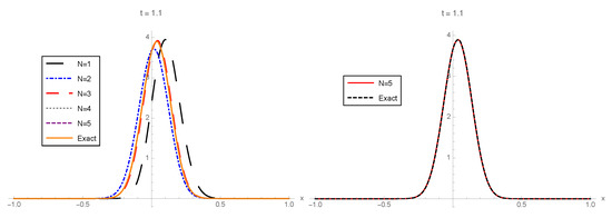
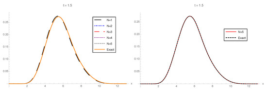
In Figure 1, Figure 2 and Figure 3, the 1-PDF of the exact solution SP, , and the 1-PDF of the truncation, , are plotted, respectively, for different values of the truncation order at the time instants . In order to graphically check the convergence, in all of these figures, we plotted the approximation corresponding to the highest order () from Expression (21) together with the exact 1-PDF. In this latter case, the 1-PDF can been obtained by applying the RVT technique from the exact representation of the solution SP given by (28), (30), and (31) and using the software Mathematica. From this latter plot, we can observe in the three cases () that and , with , practically coincide, so illustrating quick convergence. For the sake of completeness, in Table 1, we show the values of the error measure , defined in (32), which has been calculated for each using different orders of truncation :
Figure 1.
Left: 1-PDF, , of the truncated solution stochastic process (SP), , to the random initial value problem (IVP) (27) taking as the order of truncation and the corresponding 1-PDF, , of the exact solution SP at . Right: To facilitate the comparison, , with , is plotted together with . Example 1.
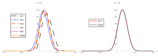
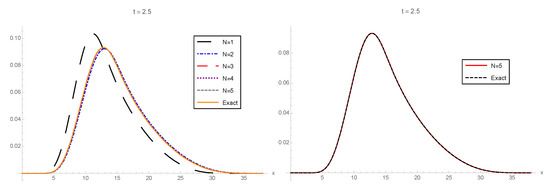
Figure 2.
Left: 1-PDF, , of the truncated solution SP, , to the random IVP (27) taking as the order of truncation and the corresponding 1-PDF, , of the exact solution SP at . Right: To facilitate the comparison, , with , is plotted together with . Example 1.
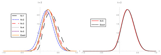
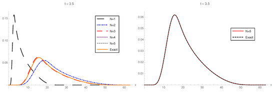
Figure 3.
Left: 1-PDF, , of the truncated solution SP, , to the random IVP (27) taking as the order of truncation and the corresponding 1-PDF, , of the exact solution SP at . Right: To facilitate the comparison, , with , is plotted together with . Example 1.
Table 1.
Error measure defined by (32) for different time instants, , and orders of truncation of the approximate solution SP, . Example 1.
From values collected in Table 1, we observe that for N fixed, the error increases as t goes far from the initial value (except for since the approximations are still rough), while for t fixed, the error decreases as the order of truncation N increases, as expected.
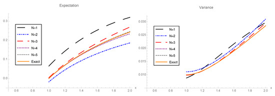
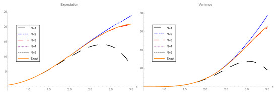
In Figure 4, we compare the expectation and the variance of the exact solution SP in the interval with the corresponding approximations for different orders of truncation, . We measure the accuracy of the approximations for these two moments via the errors defined in (33),
Figure 4.
Left: Comparison of the exact mean and the mean different approximations of the solution SP to the random IVP (27) taking as orders of truncation for the approximate series the values . Right: Comparison of exact variance and the variance different approximations of the solution SP to the random IVP (27) using the same orders of truncation. Example 1.
In Table 2, we collect the values for theses errors. For both moments, we observe that the corresponding error decreases as the order of truncation increases, as expected.
Table 2.
Values of errors for the mean, , and the variance , given by (33) for . Example 1.
Example 2.
In this example, we consider the randomized Bessel equation:
where and denote RVs fixed at the time instant . In [12], the authors provided sufficient conditions on the input random data (A, , and ) to extend the classical analysis for the Bessel equation to the random setting in the so-called mean squared sense [5]. In the aforementioned contribution, approximations for the mean and the variance of the solution SP to the Bessel RDE were given. In this example, we go further since, based on the results established in previous sections, we will construct approximations for the 1-PDF of the solution SP of this important RDE. To this end, let us first observe that, according to [12], the solution is given by , where , are defined by (17), being:
Hereinafter, we assume that A, , and are independent RVs with the following distributions:
- A has a gamma distribution with shape and scale parameters and , respectively, truncated on the interval , i.e., .
- has a beta distribution with parameters and , i.e.,
- has a uniform distribution on the interval , i.e., .
Similarly to Example 1, we first check that Hypotheses H0–H3 are fulfilled:
- H0: Since A is a truncated RV on the interval , A is bounded. With the notation of Hypothesis H0, notice that we can take, for instance, .
- H1: Since A, , and are assumed to be independent RVs, their joint PDF is given by the product of the PDF of each RV,From this expression, it is clear that this function is continuous with respect to its second argument, , and it is bounded. As we deal with a rectangular domain where the first factor is a decreasing function and the second factor, , has a maximum value at below , the maximum of is obtained taking this value and evaluating the first factor at . Therefore, with the notation of H1, we can take, for instance, . Therefore, Hypothesis H1 is fulfilled.
- H2: Notice that is a regular-singular point of the Bessel RDE (34). On the one hand, observe that according to Equation (2), , , and , being . On the other hand, according to (4) and (5), and , which are not analytic functions at , while and are both analytic at inasmuch as they are polynomials as functions of t, for every , .
- H3: Since A and are assumed to be independent RVs, then the domain of the random vector is:Hence, is a Lebesgue measurable set of , and with the notation of Hypothesis H3, we can take . Therefore, Hypothesis H3 holds.
The 1-PDFs of the truncated solution SP, , for different orders of truncation, , at the time instants are plotted in Figure 5, Figure 6 and Figure 7, respectively. As in Example 1, using the RVT method and the exact representation of series and , defined in (35), in terms of the Bessel function integrated in Mathematica and the gamma function defined in (31), namely and , we can obtain the exact 1-PDF, . On the one hand, taking this benchmark, in the left panel of Figure 5, Figure 6 and Figure 7, we show the convergence of the approximations, , to the exact 1-PDF, , as N increases () for different values of . On the other hand, to illustrate better the convergence, in the right panel of the aforementioned figures, we show the approximations corresponding to the highest order of truncation, , , and the exact 1-PDF, . We observe that both plots overlap, thus showing quick convergence.
Figure 5.
Left: 1-PDF, , of the truncated solution SP, , to the random IVP (34) taking as the order of truncation and the corresponding 1-PDF, , of the exact solution SP at . Right: To facilitate the comparison, , with , is plotted together with . Example 2.
Figure 6.
Left: 1-PDF, , of the truncated solution SP, , to the random IVP (34) taking as the order of truncation and the corresponding 1-PDF, , of the exact solution SP at . Right: To facilitate the comparison, , with , is plotted together with . Example 2.
Figure 7.
Left: 1-PDF, , of the truncated solution SP, , to the random IVP (34) taking as the order of truncation and the corresponding 1-PDF, , of the exact solution SP at . Right: To facilitate the comparison, , with , is plotted together with . Example 2.
As in Example 1, we use the error defined in (32) to measure the quality of approximations . In Table 3, we calculated, for each , the values of this error for the following orders of truncation . Notice that for each t, the error diminishes as the order of truncation increases, while the error increases as we move far from the initial data , as expected.
Taking , given by (21), as an approximation to , in the expressions (1), we can calculate approximations for the mean () and the variance () of the solution of the random IVP (34). In Figure 8, we plotted the above-mentioned approximations on the interval for different orders of truncation, , as well as their respective exact values, and , using as the expression to the one obtained via the RVT method. In these plots, we can clearly see that the approximations quickly improve on the whole interval as N increases. To finish, we calculated the errors of these approximations by means of the following expressions:
Values of errors for the mean, , and the variance, , for each truncation are shown in Table 4. From these values, we observe that errors decrease as N increases.
Table 4.
Values of errors for the approximations of mean, , and the variance, , given by (36) for . Example 2.
5. Conclusions
In this paper, we presented a methodology to construct reliable approximations to the first probability density function of the solution of second-order linear differential equations about a regular-singular point with a finite degree of randomness in the coefficients and also assuming that both initial conditions were random variables. Therefore, we studied this class of differential equations assuming randomness in all its input data, which provided great generality to our analysis. The results completed the ones already presented in a previous paper where the same class of random initial value problems was solved about an ordinary point. In this manner, the results obtained in both contributions permitted solving, from a probabilistic standpoint, a number of important randomized differential equations that appear in the field of mathematical physics like Airy, Hermite, Legendre, Laguerre, Chebyshev, Bessel, etc. Under our approach, we could compute the first probability density function of the solution. This is really advantageous since apart from allowing us to determine the mean and the variance, the knowledge of the first probability density function also permits determining higher one-dimensional moments, as well as the probability that the solution lies in any interval of interest, which might be key information in many practical problems.
Author Contributions
Formal analysis, J.-C.C, A.N.-Q., J.-V.R. and M.-D.R.; Investigation, J.-C.C., A.N.-Q., J.-V.R. and M.-D.R.; Methodology, J.-C.C., A.N.-Q., J.-V.R. and M.-D.R.; Writing – original draft, J.-C.C., A.N.-Q., J.-V.R. and M.-D.R. All authors have read and agreed to the published version of the manuscript.
Funding
This work was partially funded by the Ministerio de Economía y Competitividad Grant MTM2017-89664-P. Ana Navarro Quiles acknowledges the funding received from Generalitat Valenciana through a postdoctoral contract (APOSTD/2019/128). Computations were carried out thanks to the collaboration of Raúl San Julián Garcés and Elena López Navarro granted by the European Union through the Operational Program of the European Regional Development Fund (ERDF)/European Social Fund (ESF) of the Valencian Community 2014–2020, Grants GJIDI/2018/A/009 and GJIDI/2018/A/010, respectively.
Conflicts of Interest
The authors declare no conflict of interest.
Appendix A. Computing the solution of IVP (27) in Example 1
For the sake of completeness, in this Appendix, we detail how to obtain the expressions (28) and (29) used in Example 1. Let us consider the deterministic differential equation:
It is clear that the time instant is a regular-singular point. The indicial equation associated with the differential Equation (A1) is given by:
The solution of (A1) is sought in the form of generalized power series, , , where coefficients are determined by imposing that this series is a solution provided . This leads to the following relationship:
We work out with the last expression, obtaining:
In this last expression, we can take out the common factor , obtaining the following expression:
Now, using the uniqueness of the expansion, one gets (for the first addend), which corresponds to indicial Equation (A2), since and the following recurrence relationship derived from the other terms:
The roots of the indicial Equation (A2) are and , then according to the Fröbenius method stated in Theorem 1, if and is not an integer, differential Equation (A1) has two linearly independent solutions of the form:
where terms and are obtained from the recurrence (A3) with and , respectively, for fixed. Taking , one recursively calculates:
References
- Hussein, A.; Selim, M.M. Solution of the stochastic radiative transfer equation with Rayleigh scattering using RVT technique. Appl. Math. Comput. 2012, 218, 7193–7203. [Google Scholar] [CrossRef]
- Dorini, F.A.; Cecconello, M.S.; Dorini, M.B. On the logistic equation subject to uncertainties in the environmental carrying capacity and initial population density. Commun. Nonlinear Sci. Numer. Simul. 2016, 33, 160–173. [Google Scholar] [CrossRef]
- Santos, L.T.; Dorini, F.A.; Cunha, M.C.C. The probability density function to the random linear transport equation. Appl. Math. Comput. 2010, 216, 1524–1530. [Google Scholar] [CrossRef]
- Hussein, A.; Selim, M.M. A complete probabilistic solution for a stochastic Milne problem of radiative transfer using KLE-RVT technique. J. Quant. Spectrosc. Radiat. Transf. 2019, 232, 254–265. [Google Scholar] [CrossRef]
- Soong, T.T. Random Differential Equations in Science and Engineering; Academic Press: New York, NY, USA, 1973. [Google Scholar]
- Cortés, J.C.; Navarro-Quiles, A.; Romero, J.V.; Roselló, M.D. Solving second-order linear differential equations with random analytic coefficients about ordinary points: A full probabilistic solution by the first probability density function. Appl. Math. Comput. 2018, 331, 33–45. [Google Scholar] [CrossRef]
- Cortés, J.C.; Jódar, L.; Camacho, J.; Villafuerte, L. Random Airy type differential equations: Mean square exact and numerical solutions. Comput. Math. Appl. 2010, 60, 1237–1244. [Google Scholar] [CrossRef]
- Calbo, G.; Cortés, J.C.; Jódar, L. Random Hermite differential equations: Mean square power series solutions and statistical properties. Appl. Math. Comput. 2011, 218, 3654–3666. [Google Scholar] [CrossRef]
- Calbo, G.; Cortés, J.C.; Jódar, L. Solving the random Legendre differential equation: Mean square power series solution and its statistical functions. Comput. Math. Appl. 2011, 61, 2782–2792. [Google Scholar] [CrossRef]
- Calbo, G.; Cortés, J.C.; Jódar, L. Laguerre random polynomials: Definition, differential and statistical properties. Util. Math. 2015, 60, 283–293. [Google Scholar]
- Cortés, J.C.; Villafuerte, L.; Burgos, C. A mean square chain rule and its application in solving the random Chebyshev differential equation. Mediterr. J. Math. 2017, 14, 14–35. [Google Scholar] [CrossRef]
- Cortés, J.C.; Jódar, L.; Villafuerte, L. Mean square solution of Bessel differential equation with uncertainties. J. Comput. Appl. Math. 2017, 309, 383–395. [Google Scholar] [CrossRef]
- Golmankhaneh, A.K.; Porghoveh, N.A.; Baleanu, D. Mean square solutions of second-order random differential equations by using homotopy analysis method. Rom. Rep. Phys. 2013, 65, 350–362. [Google Scholar]
- Khalaf, S. Mean Square Solutions of Second-Order Random Differential Equations by Using Homotopy Perturbation Method. Int. Math. Forum 2011, 6, 2361–2370. [Google Scholar]
- Khudair, A.; Ameen, A.; Khalaf, S. Mean square solutions of second-order random differential equations by using Adomian decomposition method. Appl. Math. Sci. 2011, 5, 2521–2535. [Google Scholar]
- Khudair, A.; Haddad, S.; Khalaf, S. Mean Square Solutions of Second-Order Random Differential Equations by Using the Differential Transformation Method. Open J. Appl. Sci. 2016, 6, 287–297. [Google Scholar] [CrossRef][Green Version]
- Khudair, A.; Ameen, A.; Khalaf, S. Mean Square Solutions of Second-Order Random Differential Equations by Using Variational Iteration Method. Appl. Math. Sci. 2011, 5, 2505–2519. [Google Scholar]
- Ross, S.L. Differential Equations; John Willey & Sons: New York, NY, USA, 1984. [Google Scholar]
- Qi, Y. A Very Brief Introduction to Nonnegative Tensors from the Geometric Viewpoint. Mathematics 2018, 6, 230. [Google Scholar] [CrossRef]
- Ragusa, M.A.; Tachikawa, A. Boundary regularity of minimizers of p(x)-energy functionals. Ann. de l’Institut Henri Poincare (C) Non Linear Anal. 2016, 33, 451–476. [Google Scholar] [CrossRef]
- Ragusa, M.A.; Tachikawa, A. Regularity for minimizers for functionals of double phase with variable exponents. Adv. Nonlinear Anal. 2020, 9, 710–728. [Google Scholar] [CrossRef]
- Braumann, C.; Cortés, J.C.; Jódar, L.; Villafuerte, L. On the random gamma function: Theory and computing. J. Comput. Appl. Math. 2018, 335, 142–155. [Google Scholar] [CrossRef]
© 2020 by the authors. Licensee MDPI, Basel, Switzerland. This article is an open access article distributed under the terms and conditions of the Creative Commons Attribution (CC BY) license (http://creativecommons.org/licenses/by/4.0/).