Author Contributions
Conceptualization, S.A.A.K.; formal analysis, A.G. and D.B.; funding acquisition, S.A.A.K.; methodology, A.G. and K.S.N.; software, F.A.M.A., S.A.A.K., A.S., and M.K.H.; visualization, A.G.; writing—original draft, F.A.M.A., S.A.A.K., A.S., M.K.H., and K.S.N.; writing—review and editing, K.S.N. and D.B. All authors have read and agreed to the published version of the manuscript.
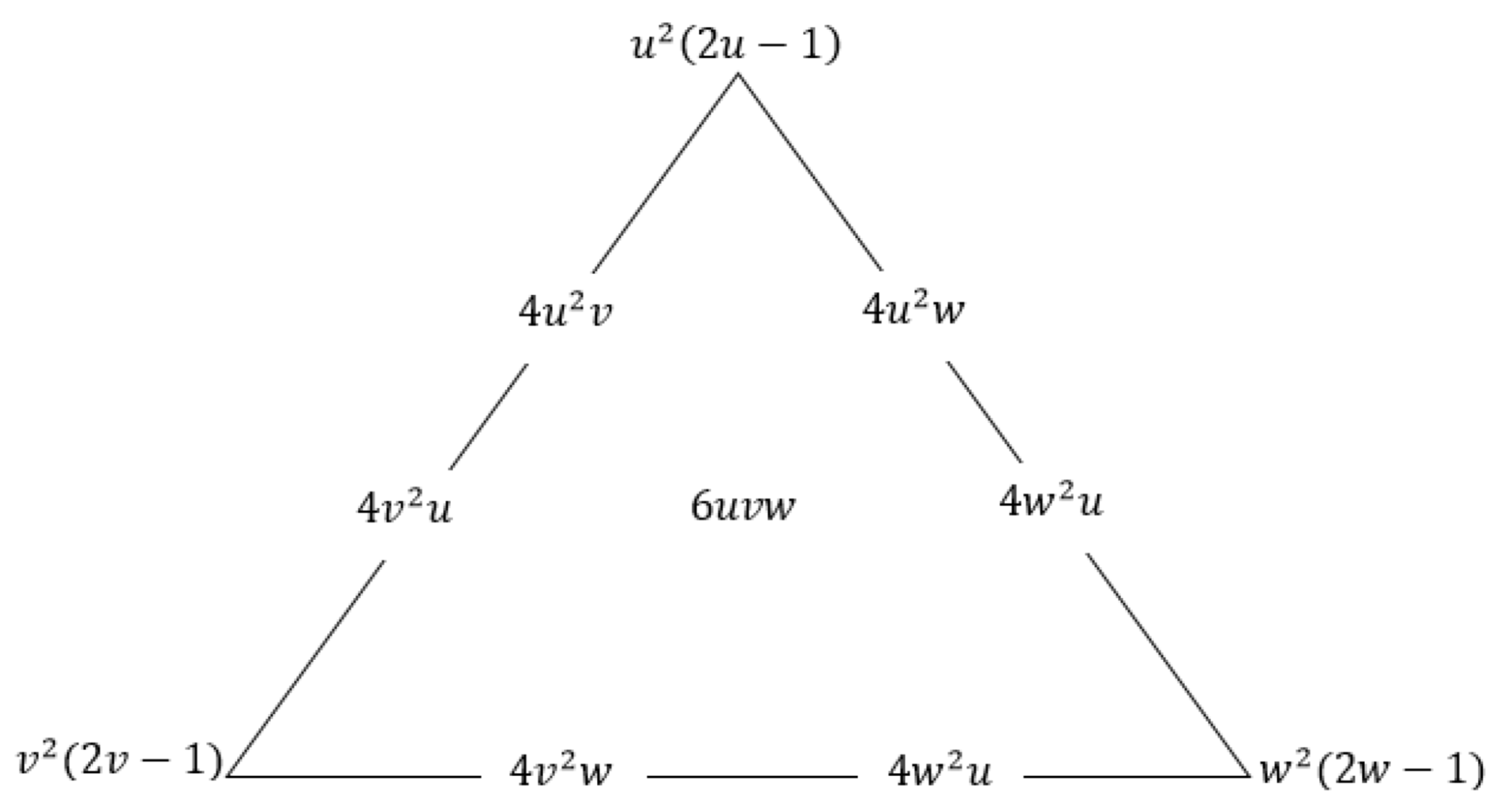
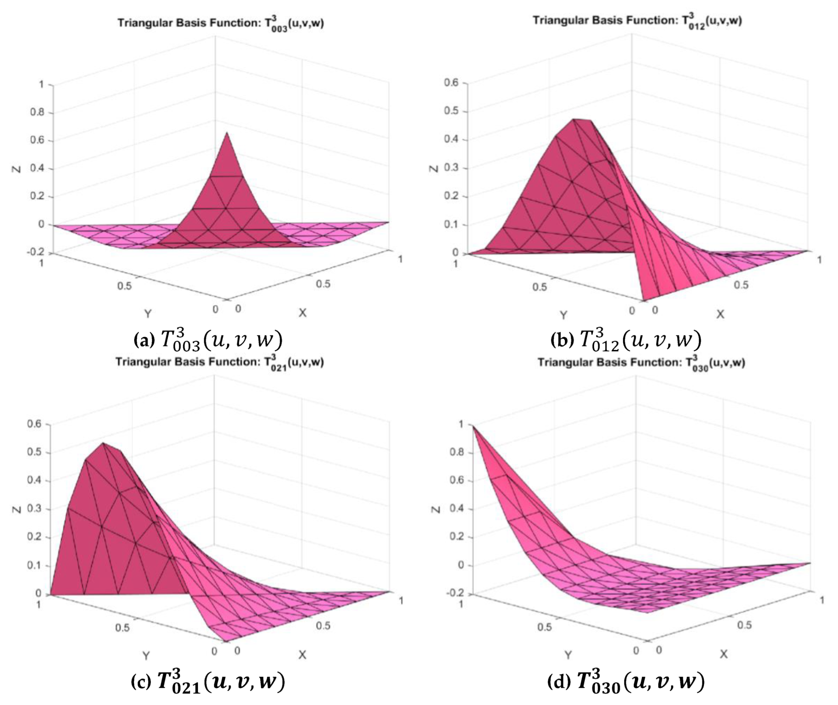
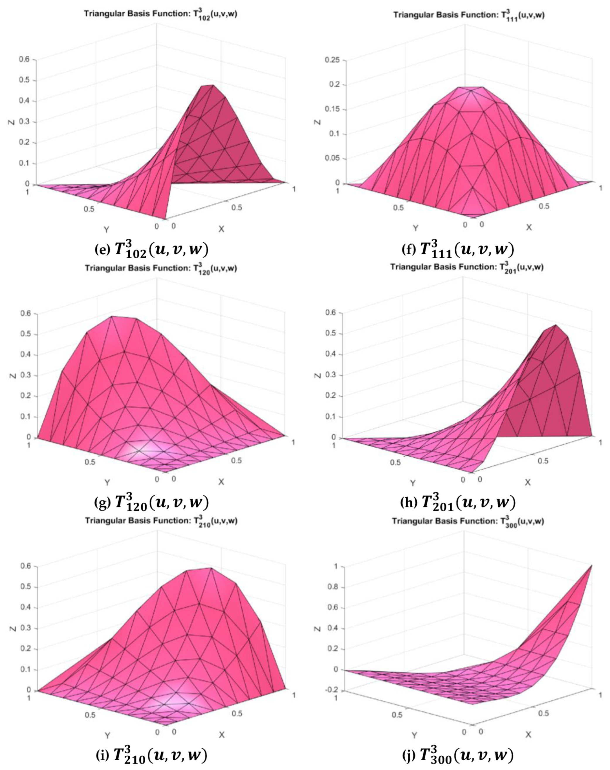
Figure 1.
Some cubic Timmer triangular basis functions.
Figure 1.
Some cubic Timmer triangular basis functions.
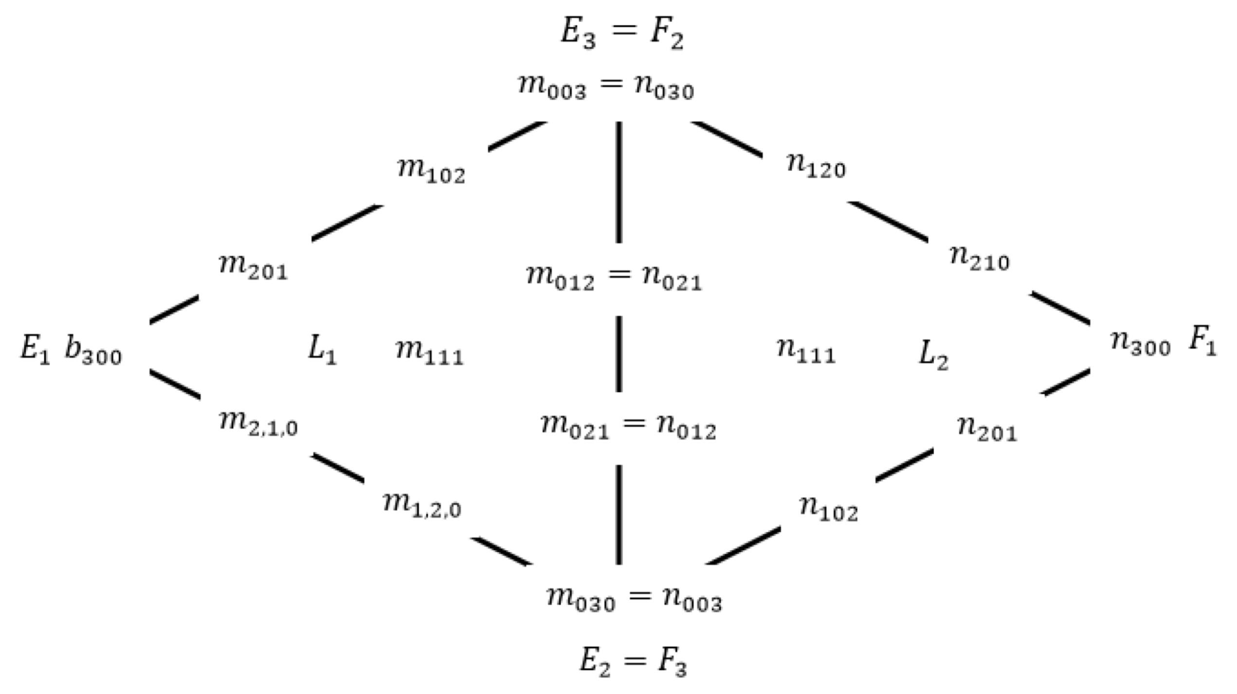
Figure 2.
Control nets for cubic Timmer triangular patch.
Figure 2.
Control nets for cubic Timmer triangular patch.
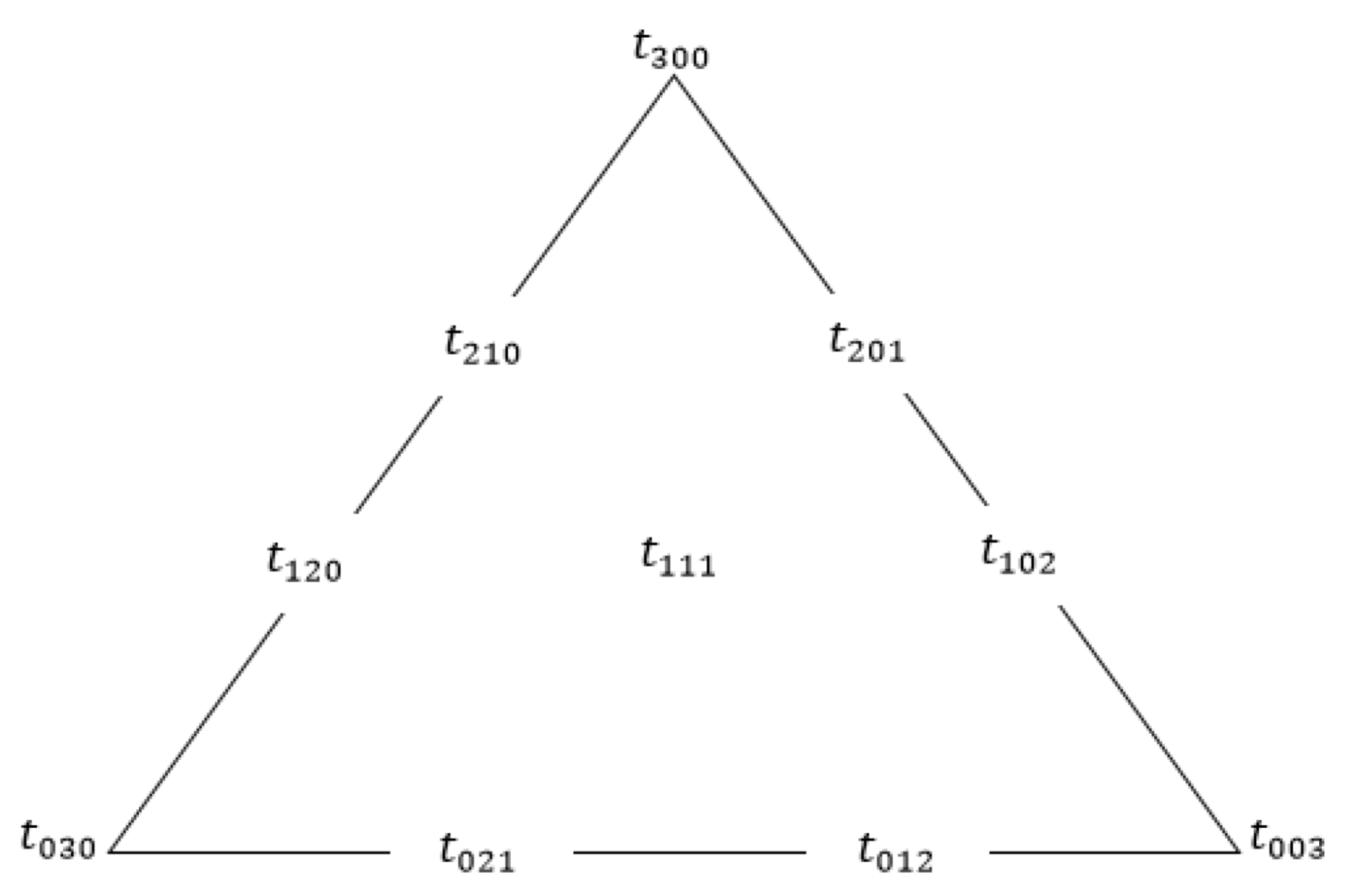
Figure 3.
Cubic Timmer triangular bases.
Figure 3.
Cubic Timmer triangular bases.
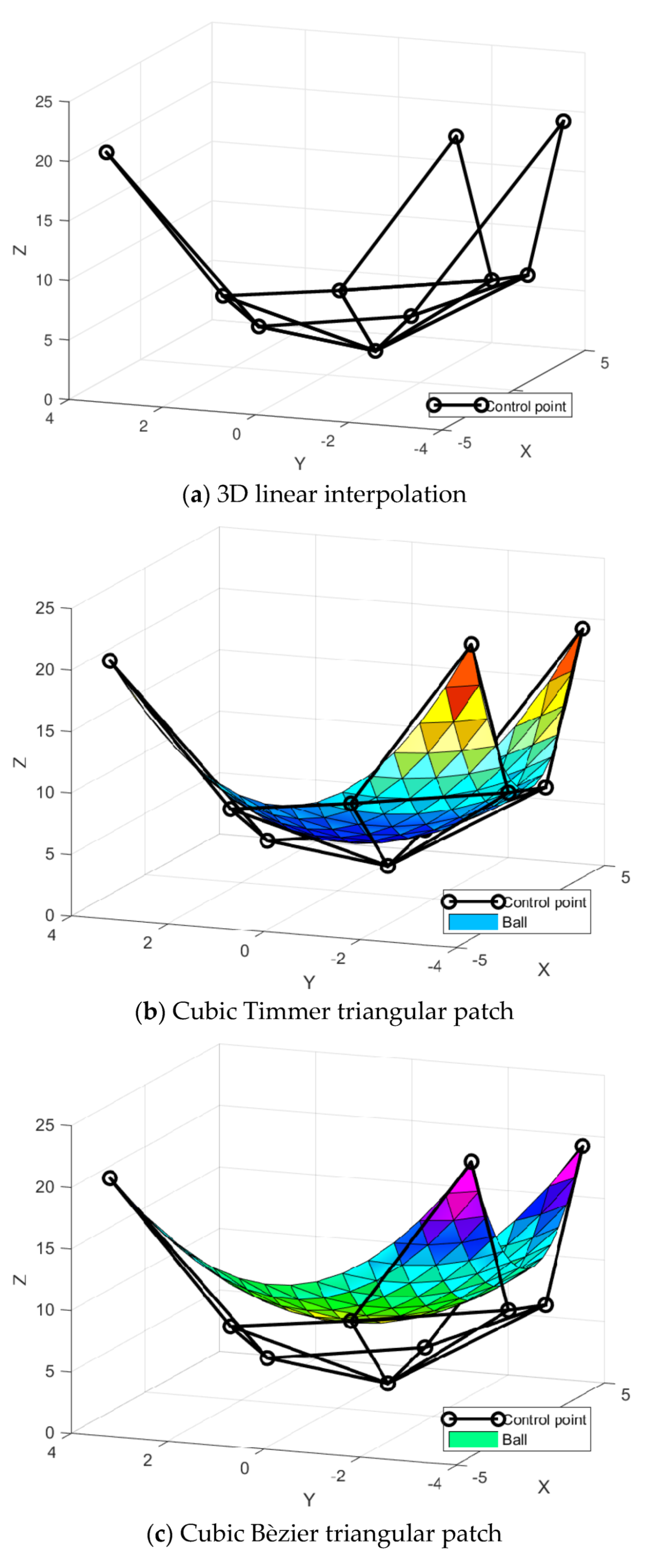
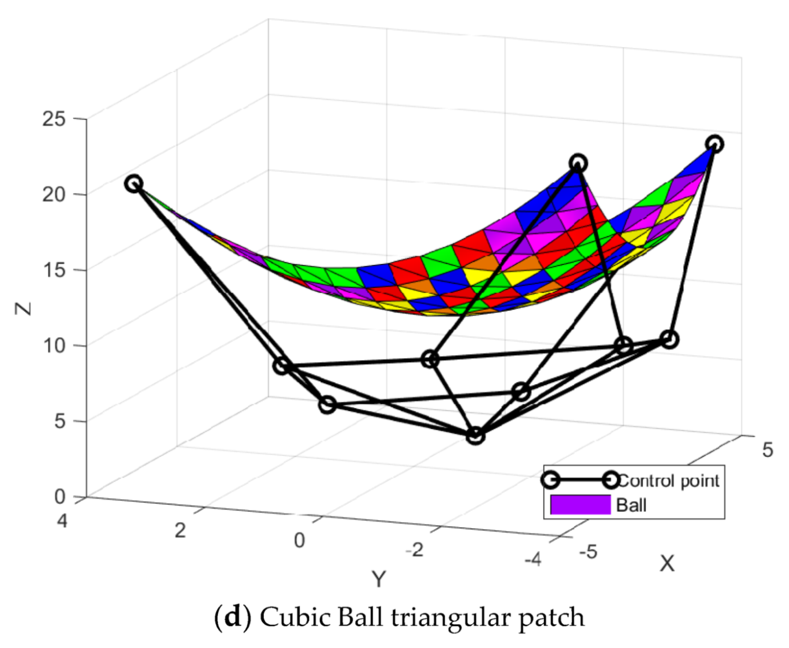
Figure 4.
Surface interpolation.
Figure 4.
Surface interpolation.
Figure 5.
Inward normal direction to the edges of triangle.
Figure 5.
Inward normal direction to the edges of triangle.
Figure 6.
Two adjacent cubic triangular patches for Foley and Opitz [
19].
Figure 6.
Two adjacent cubic triangular patches for Foley and Opitz [
19].
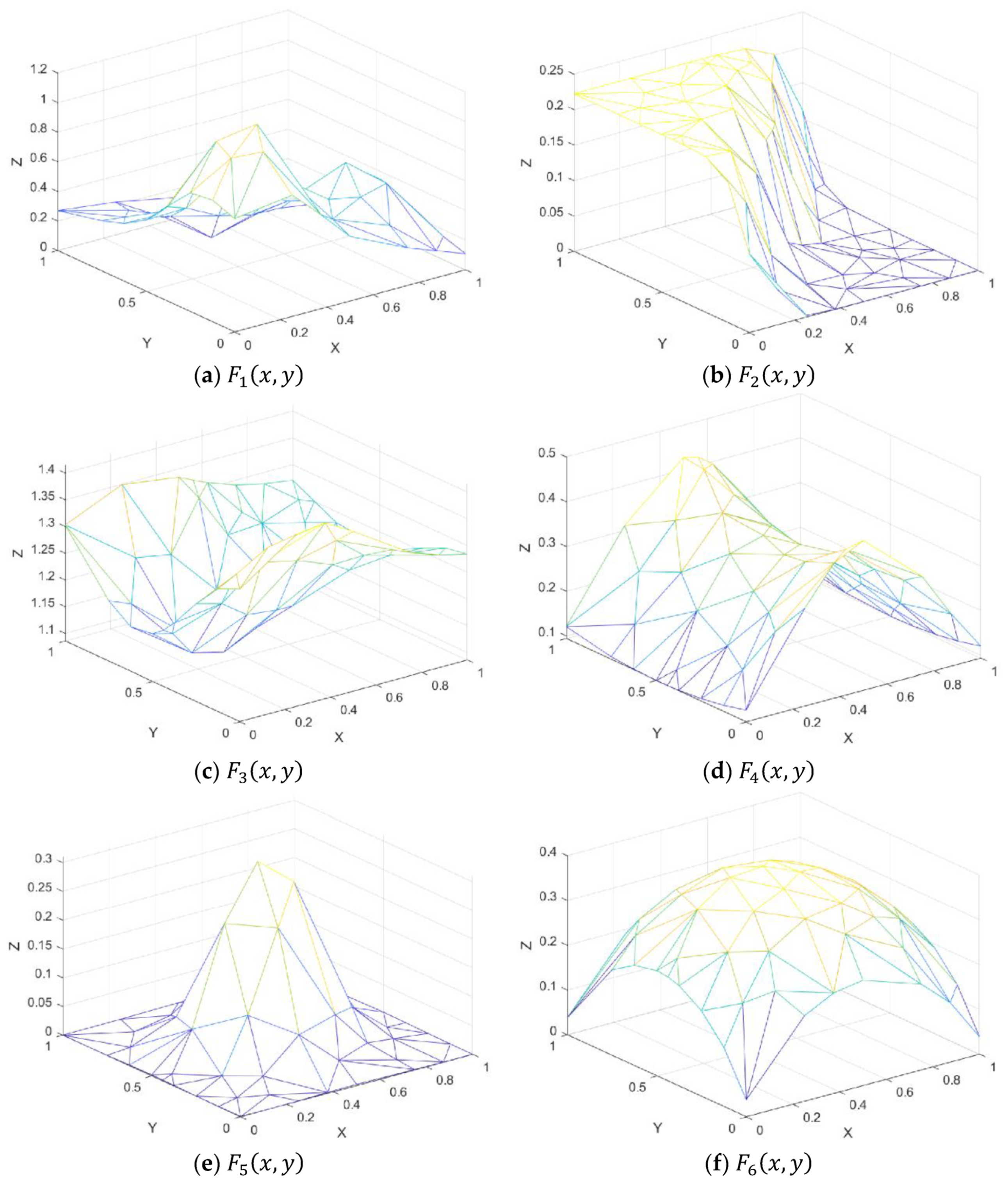
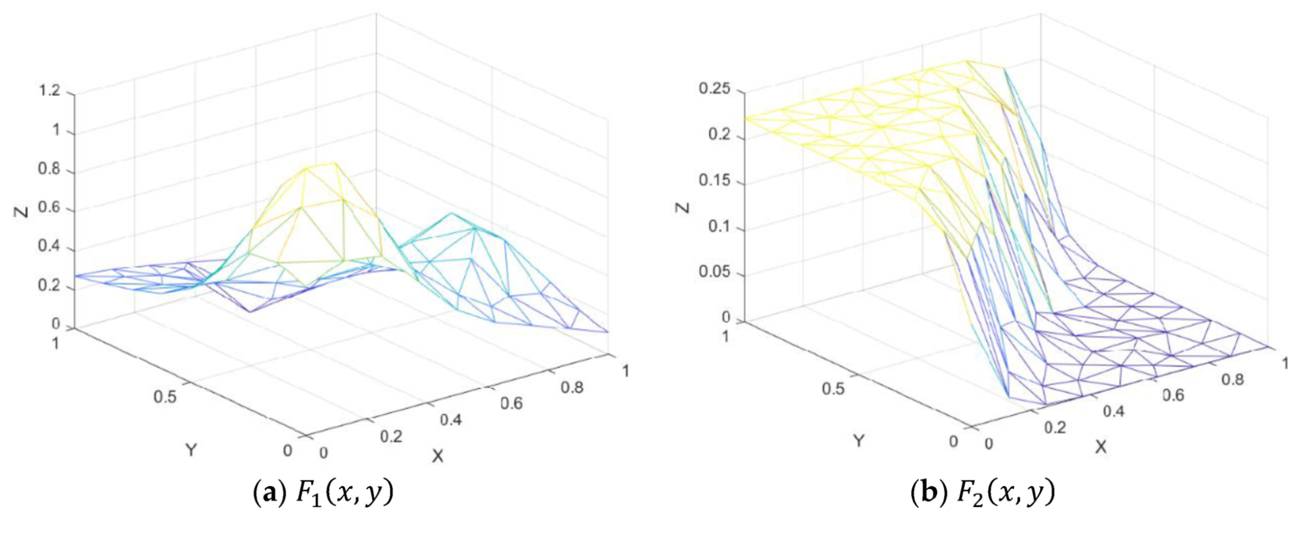
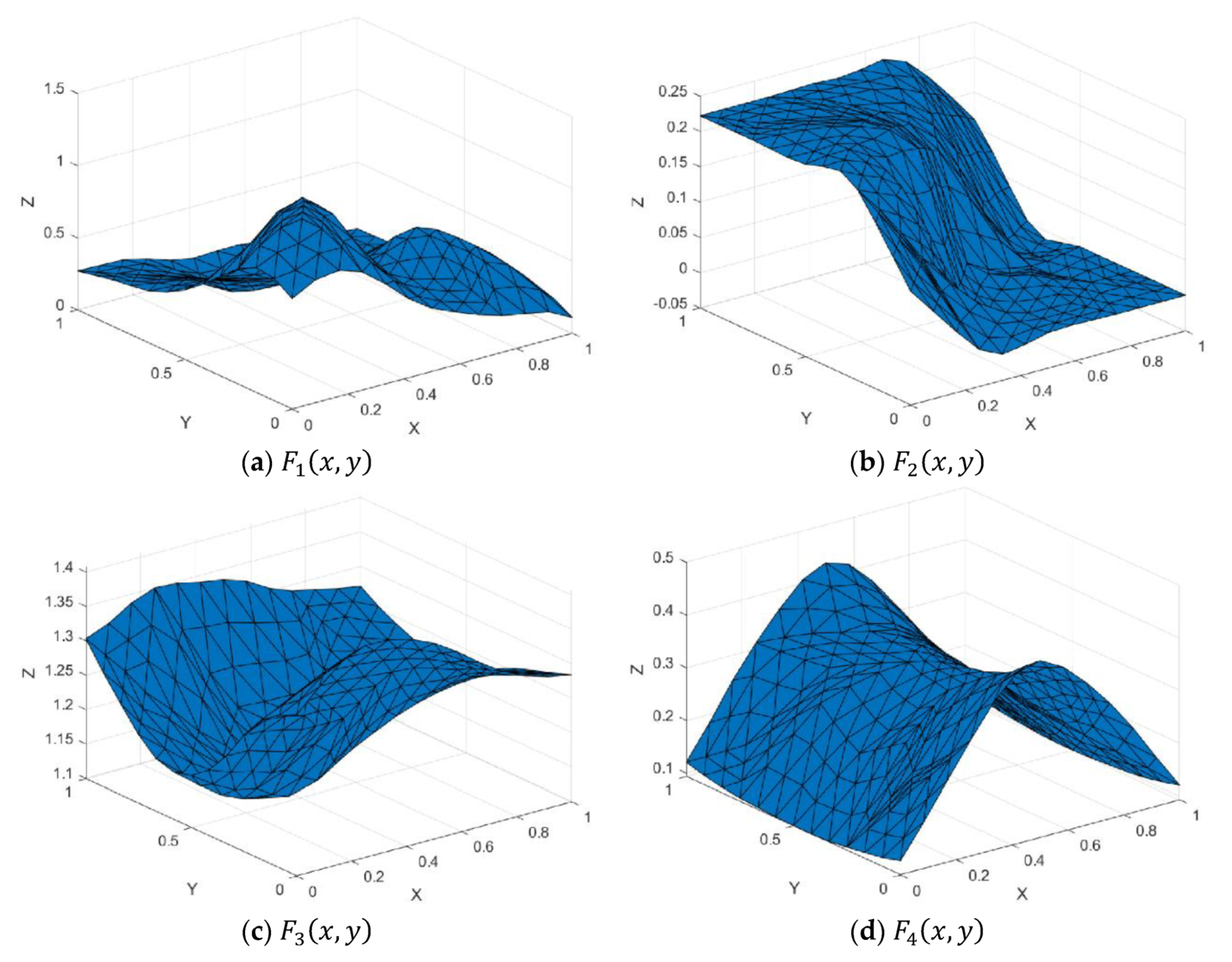
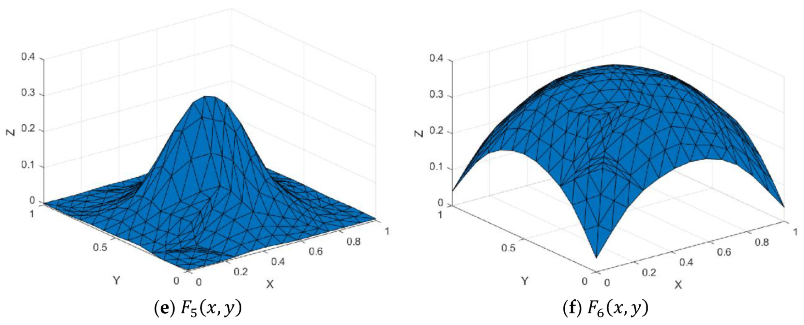
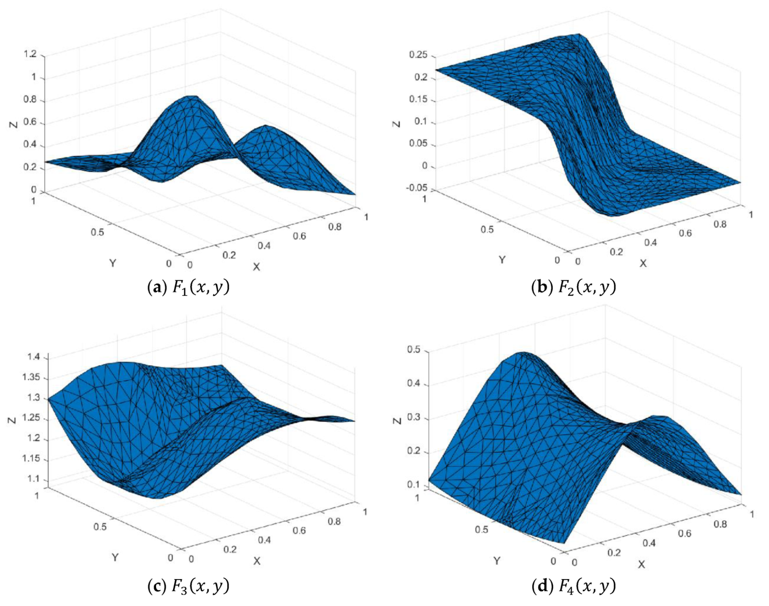
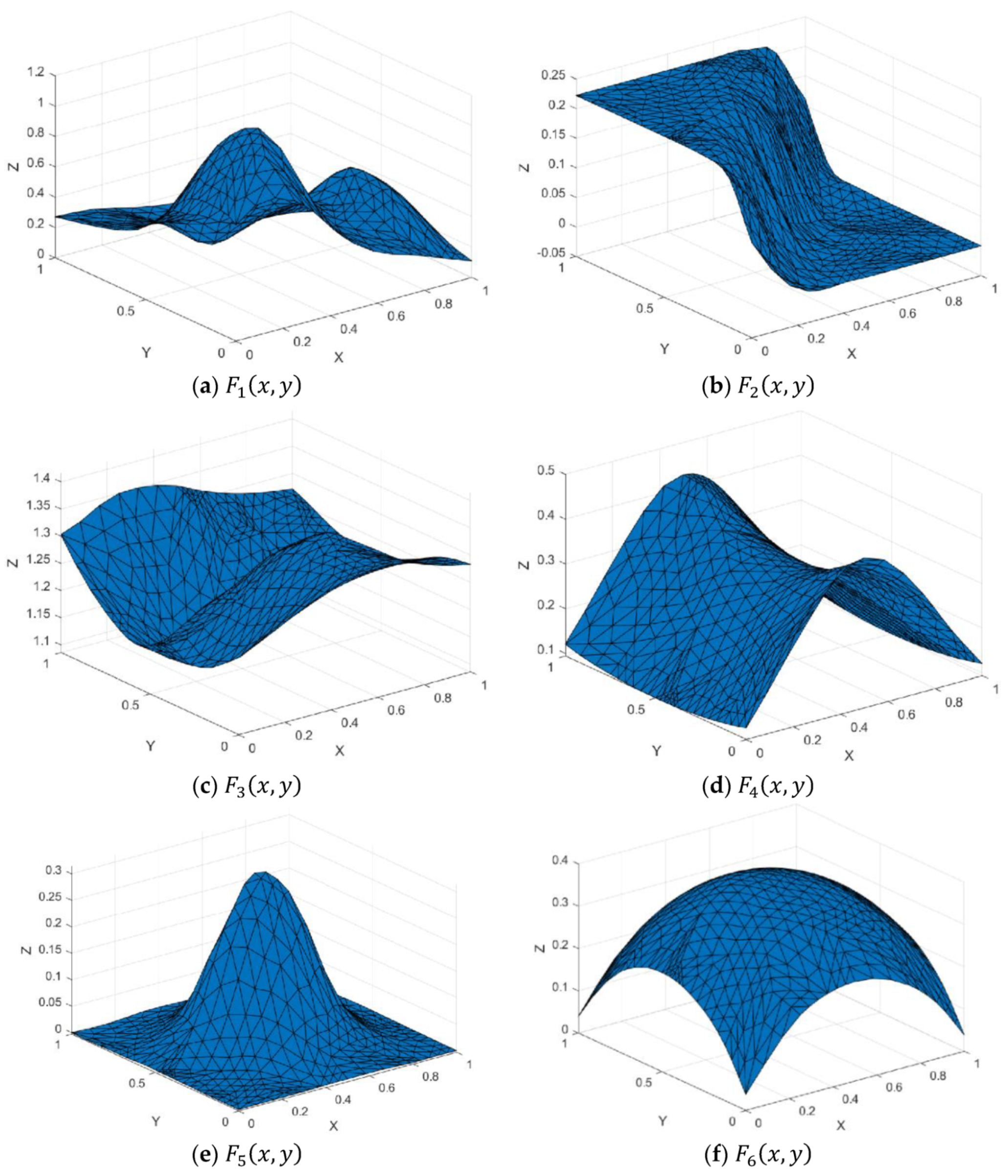
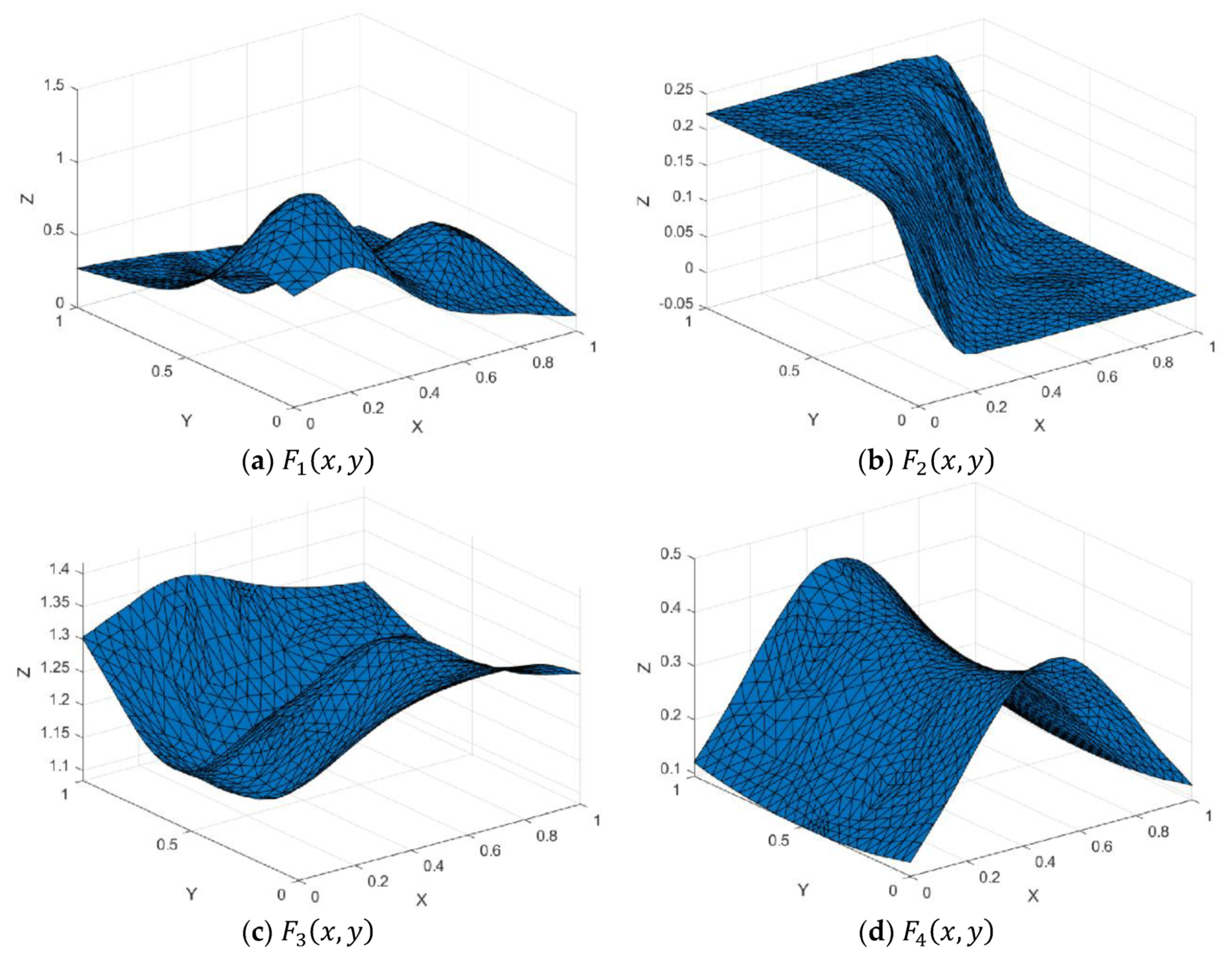
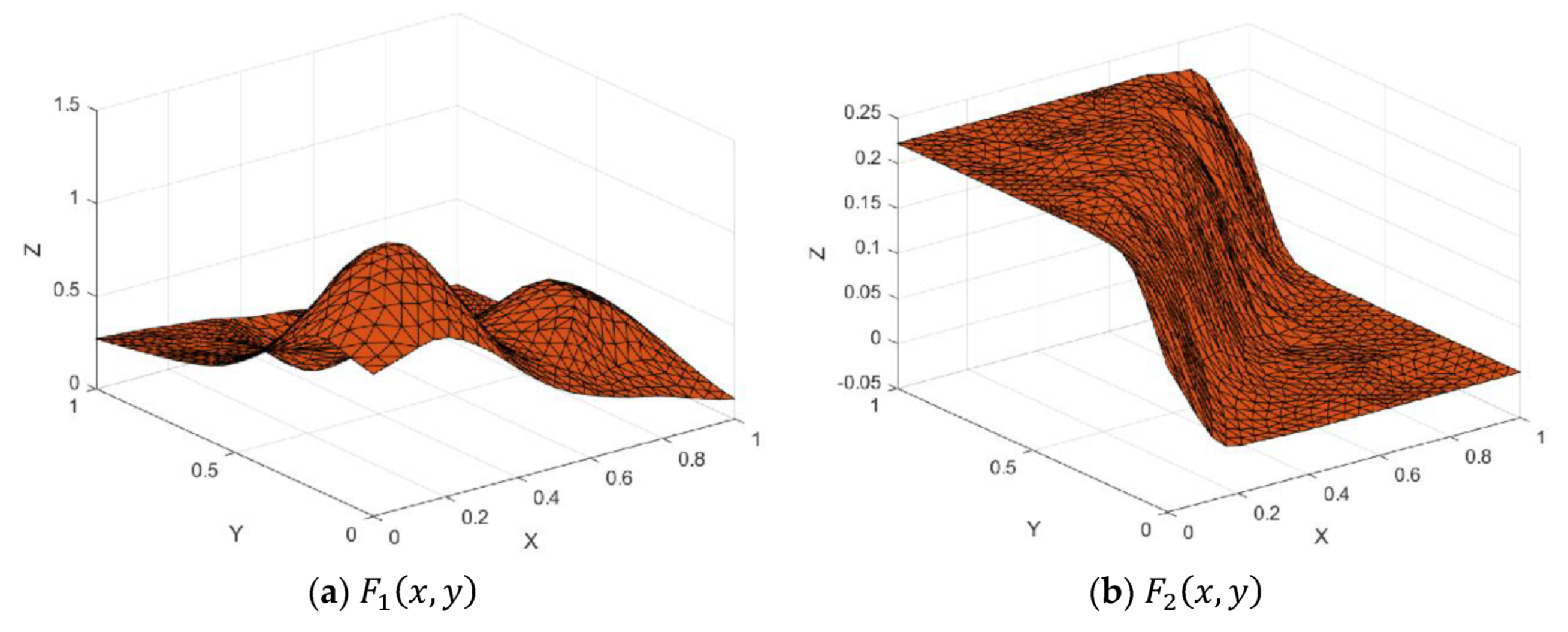
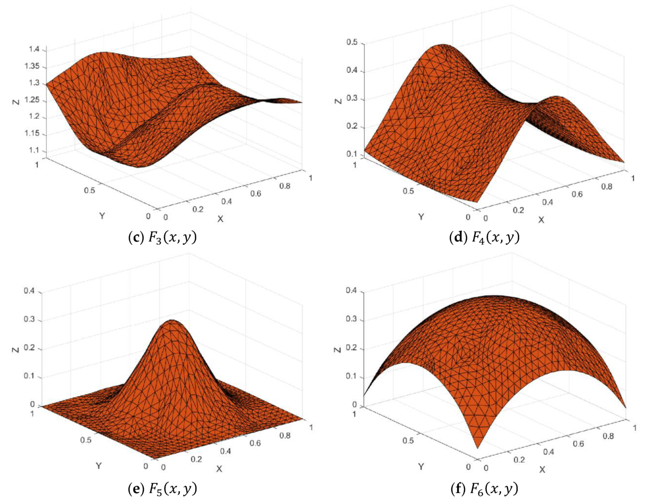
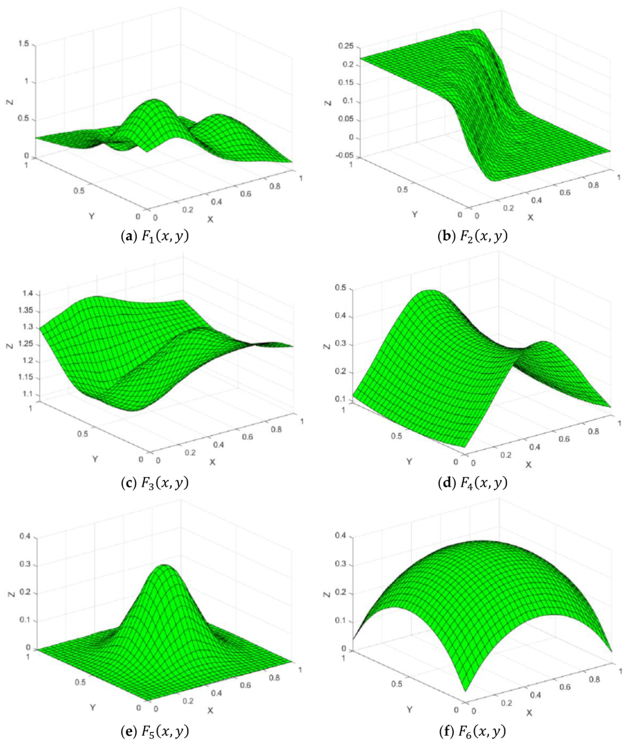
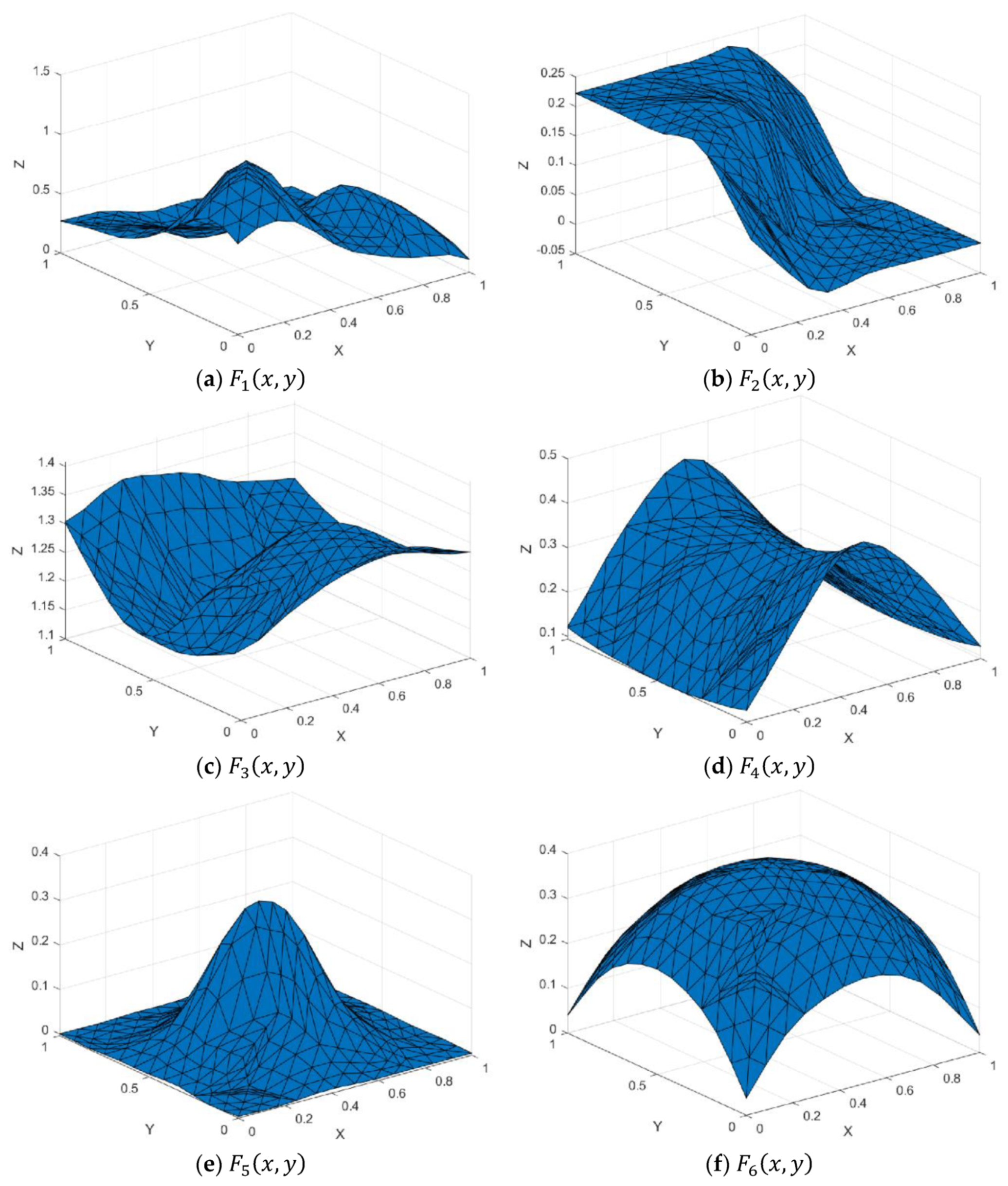
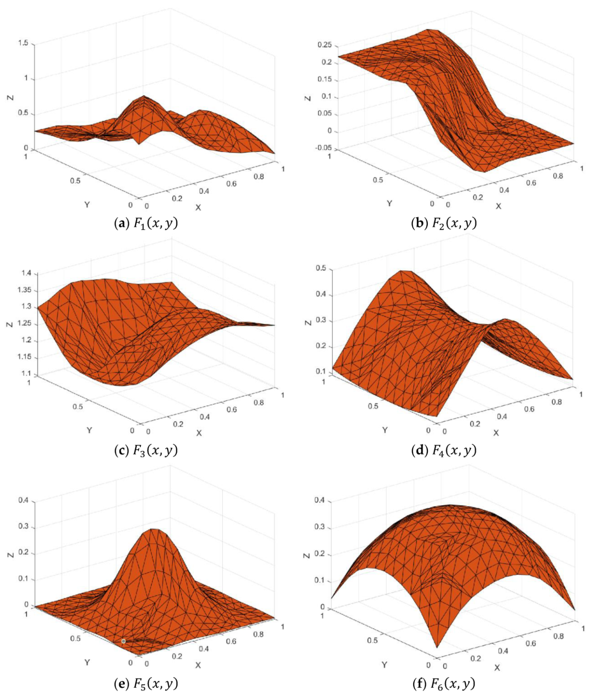
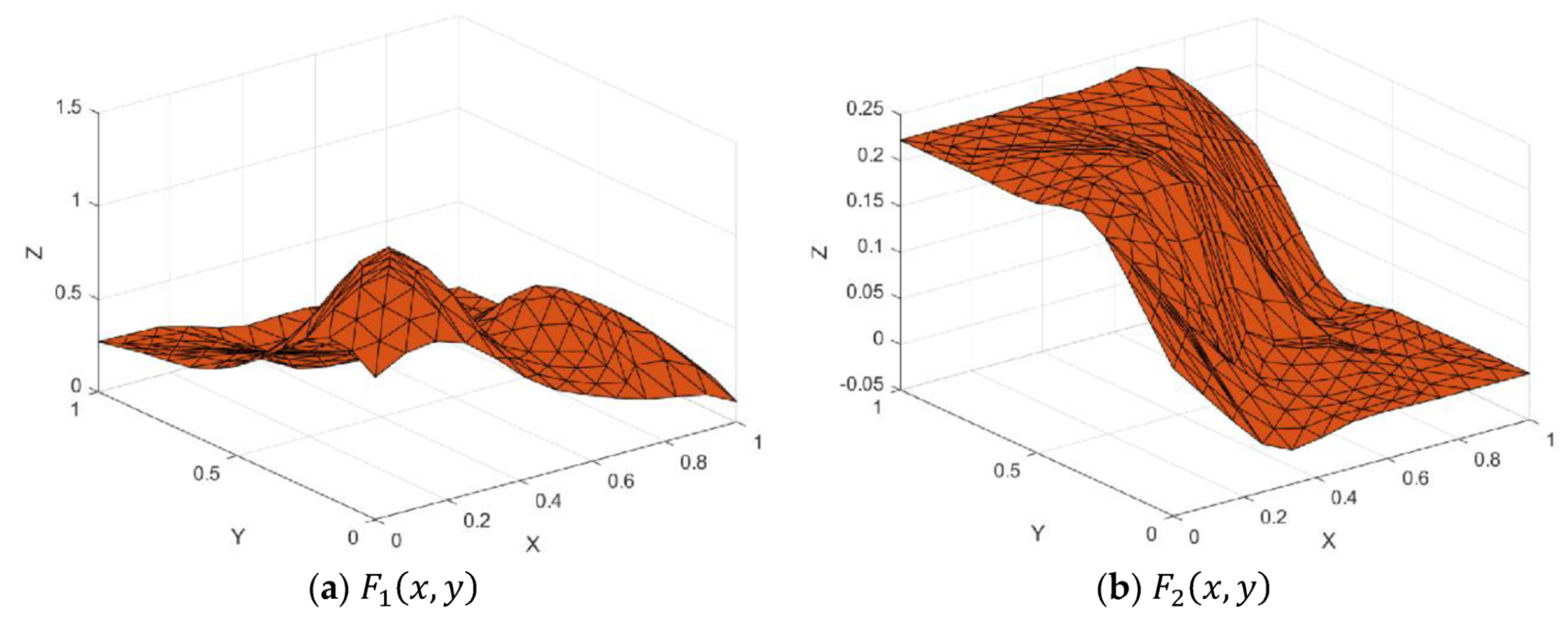
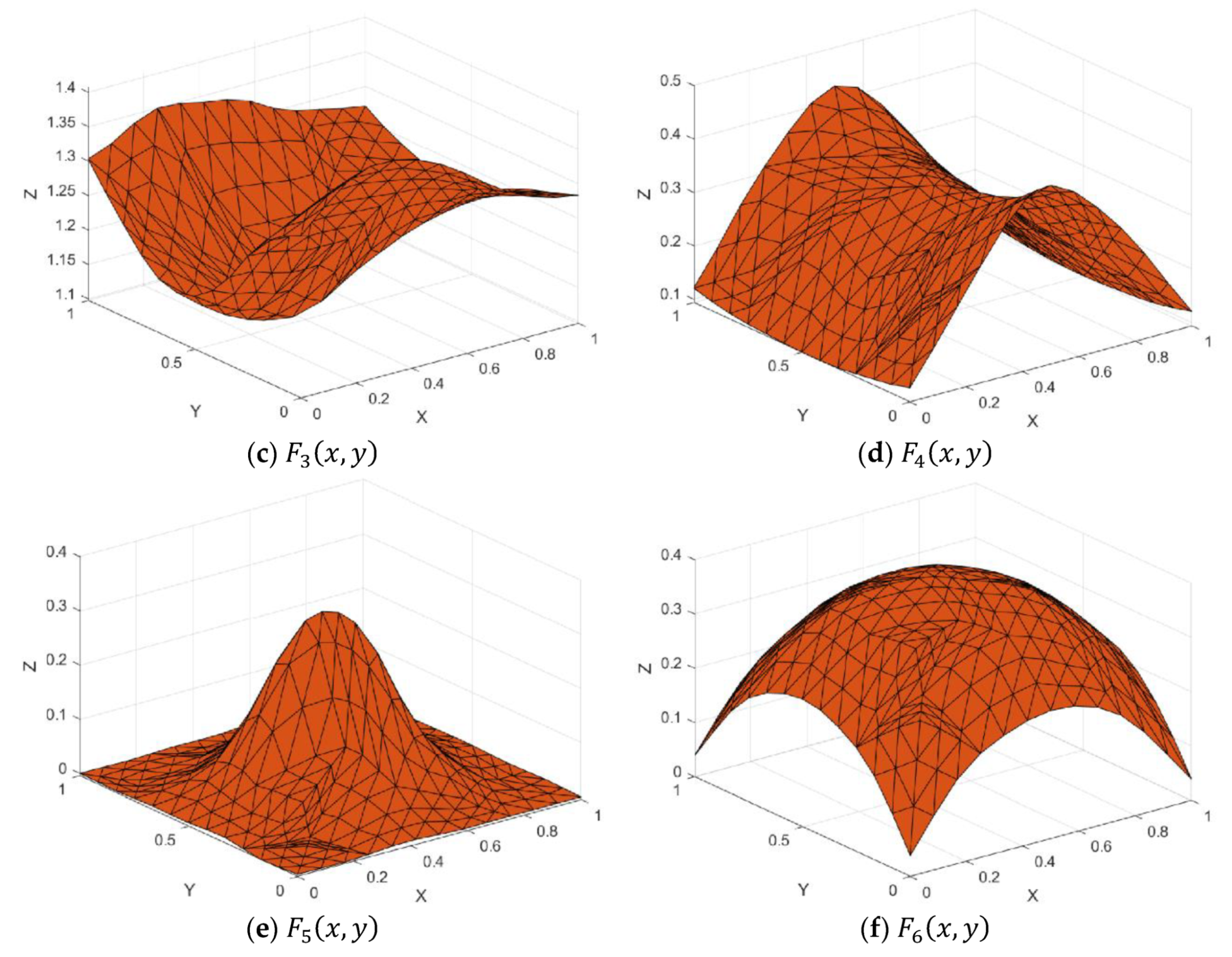
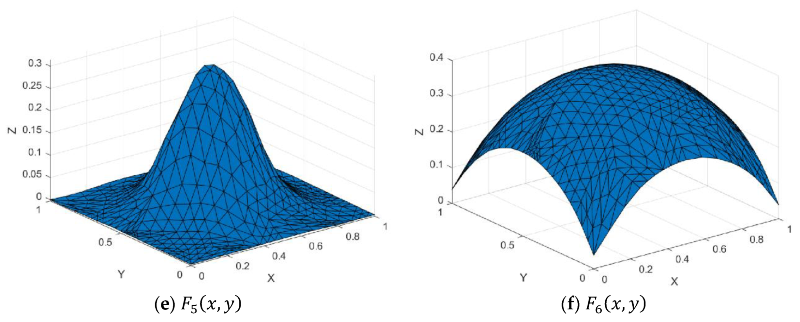
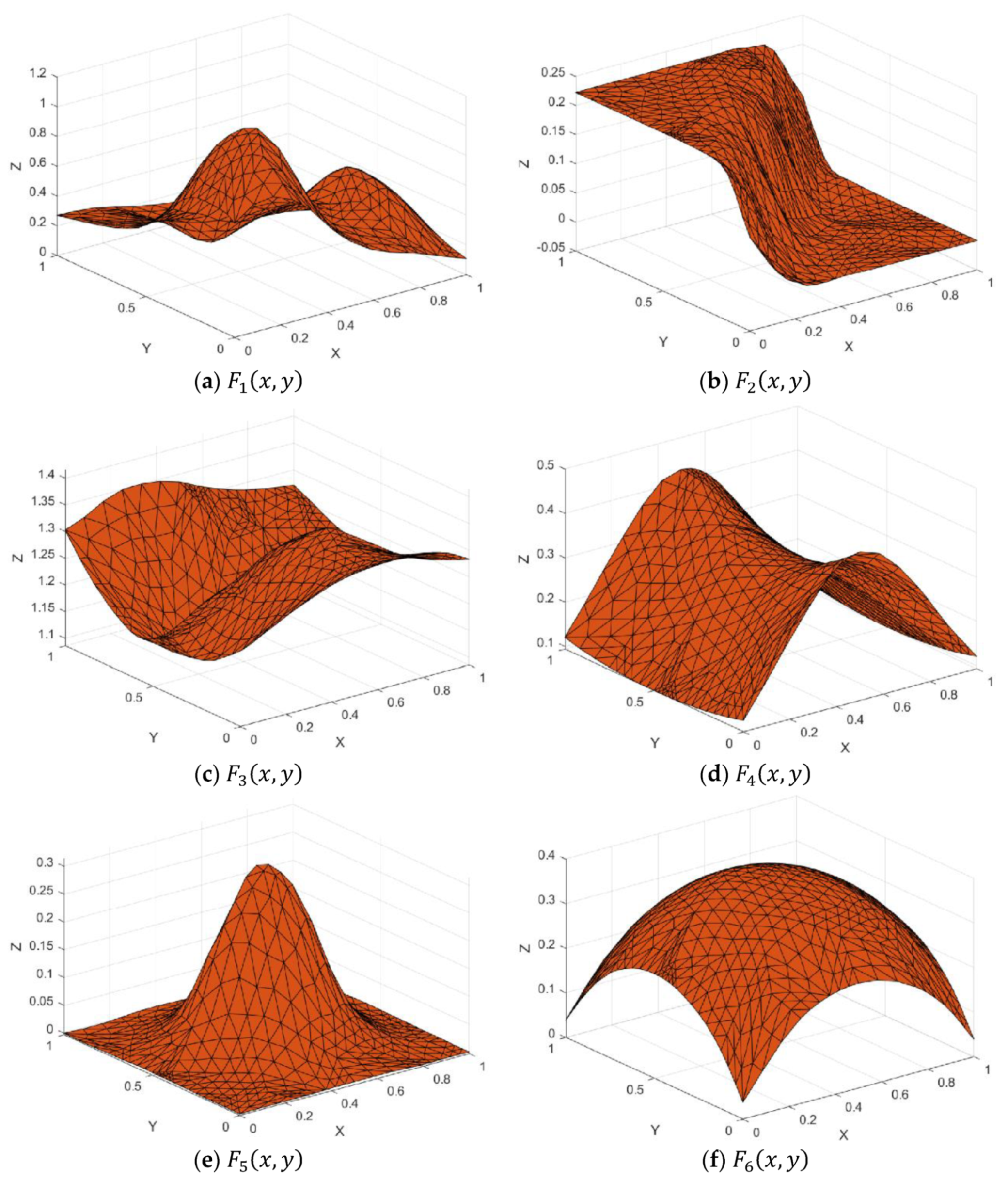
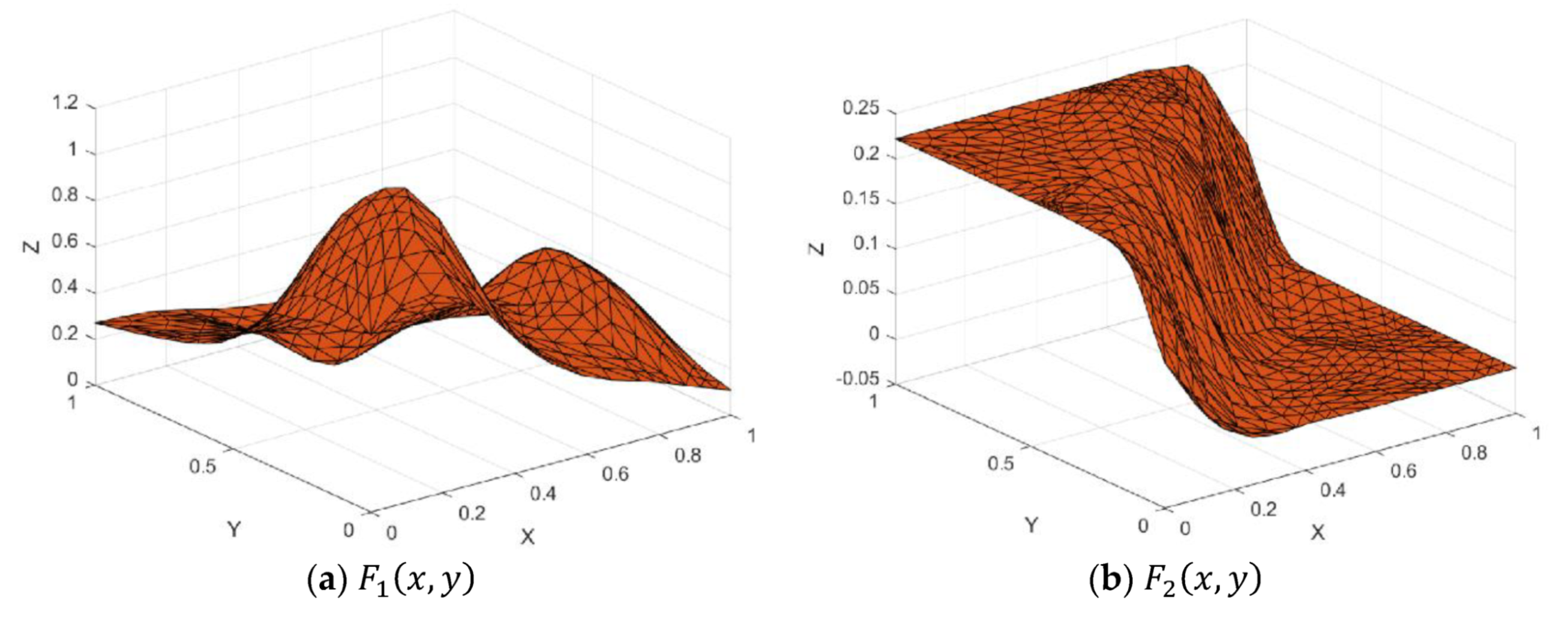
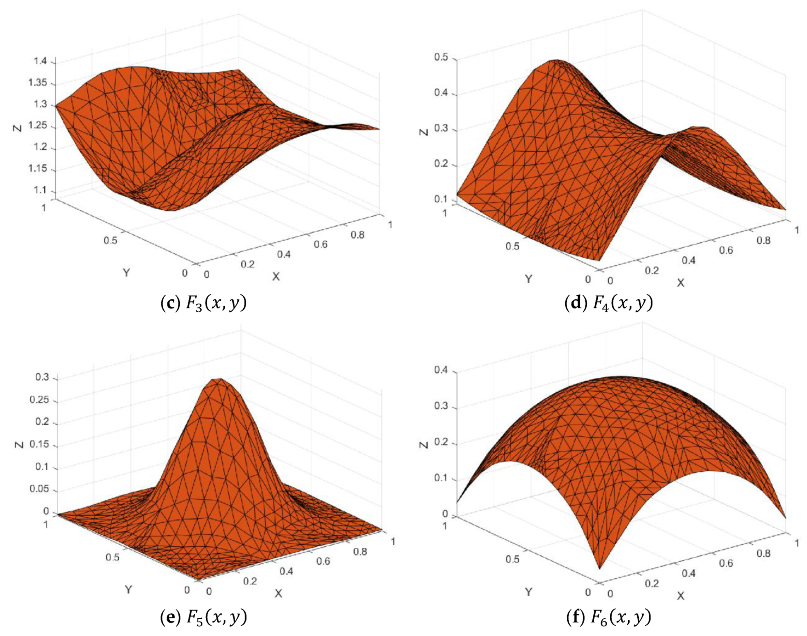
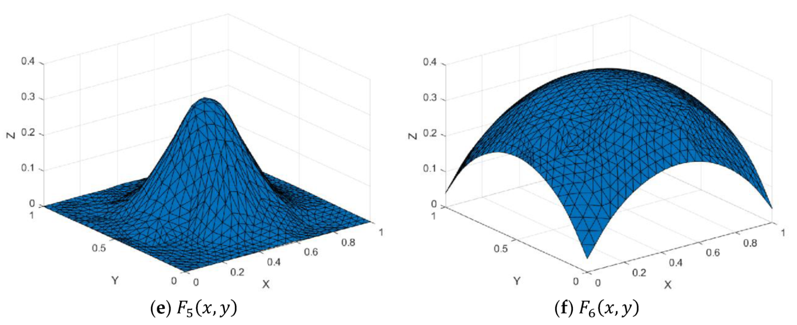
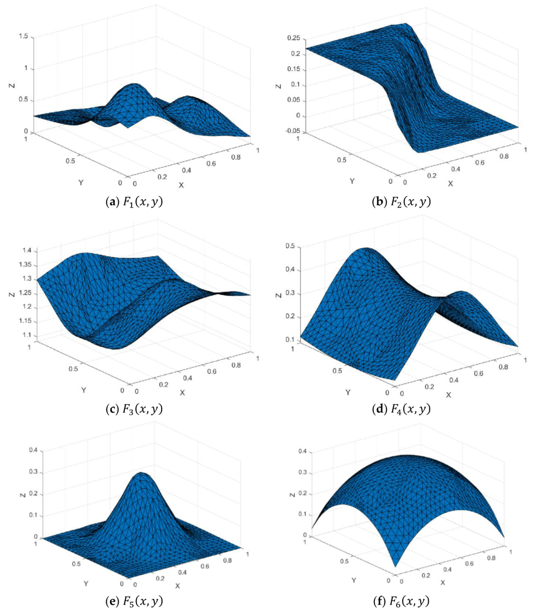
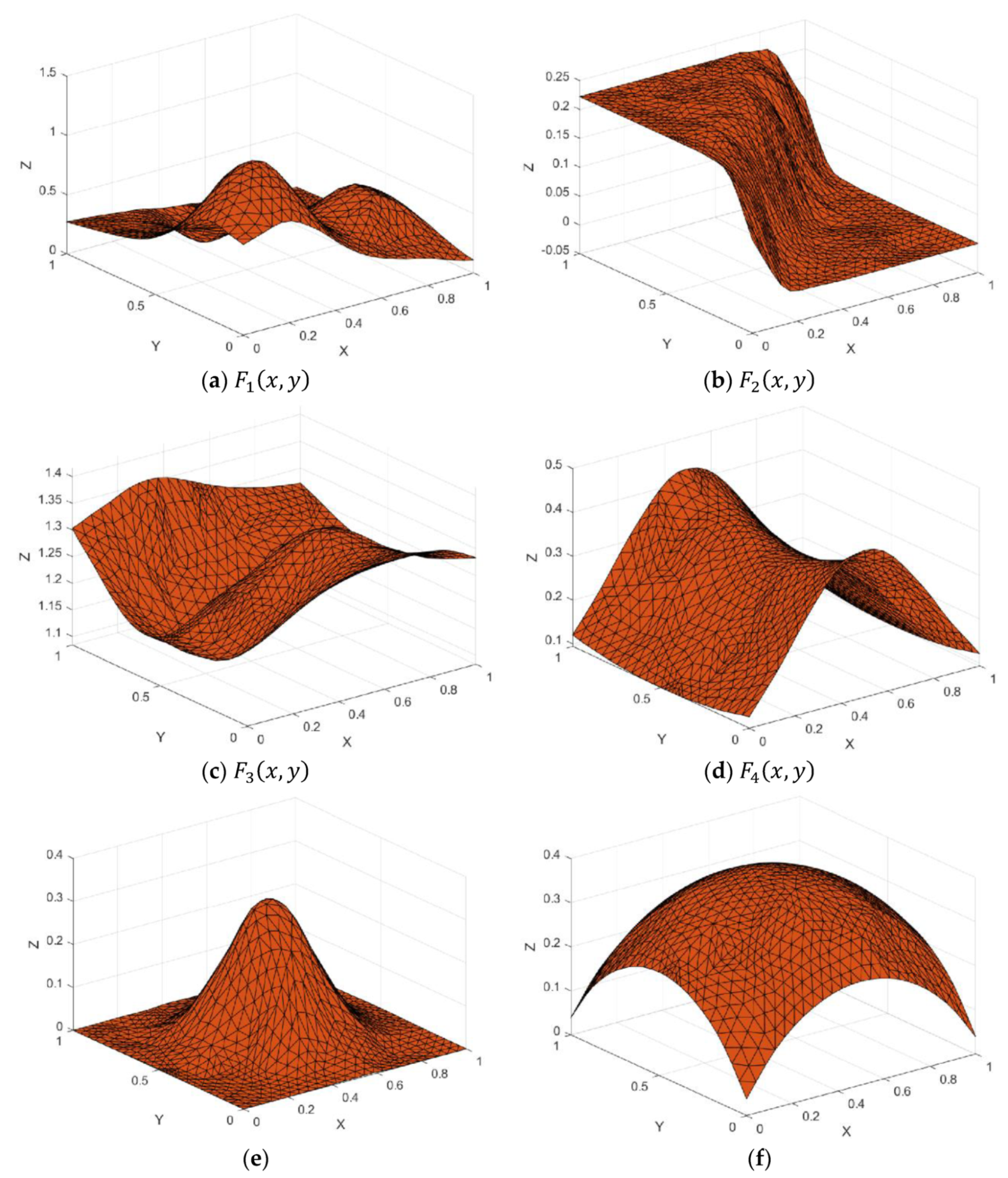
Figure 7.
Test functions.
Figure 7.
Test functions.
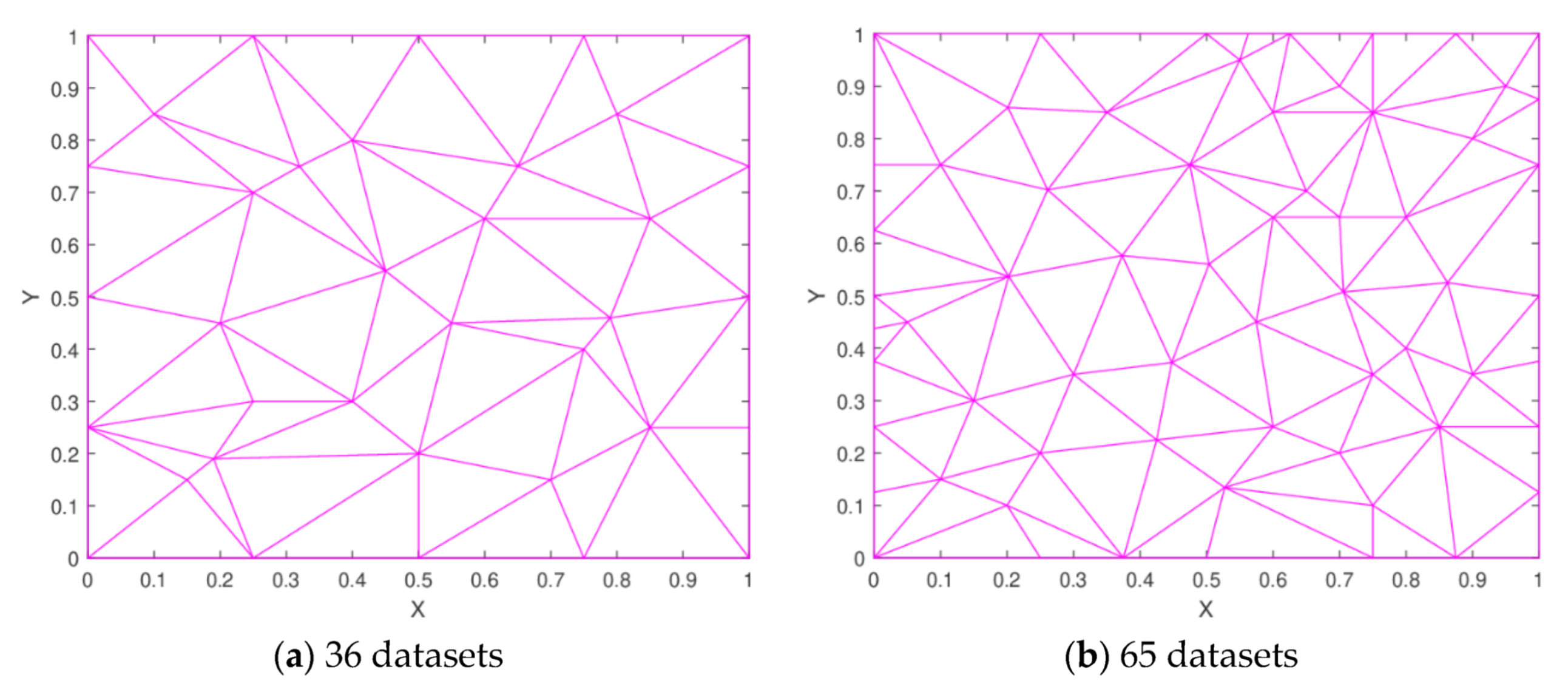
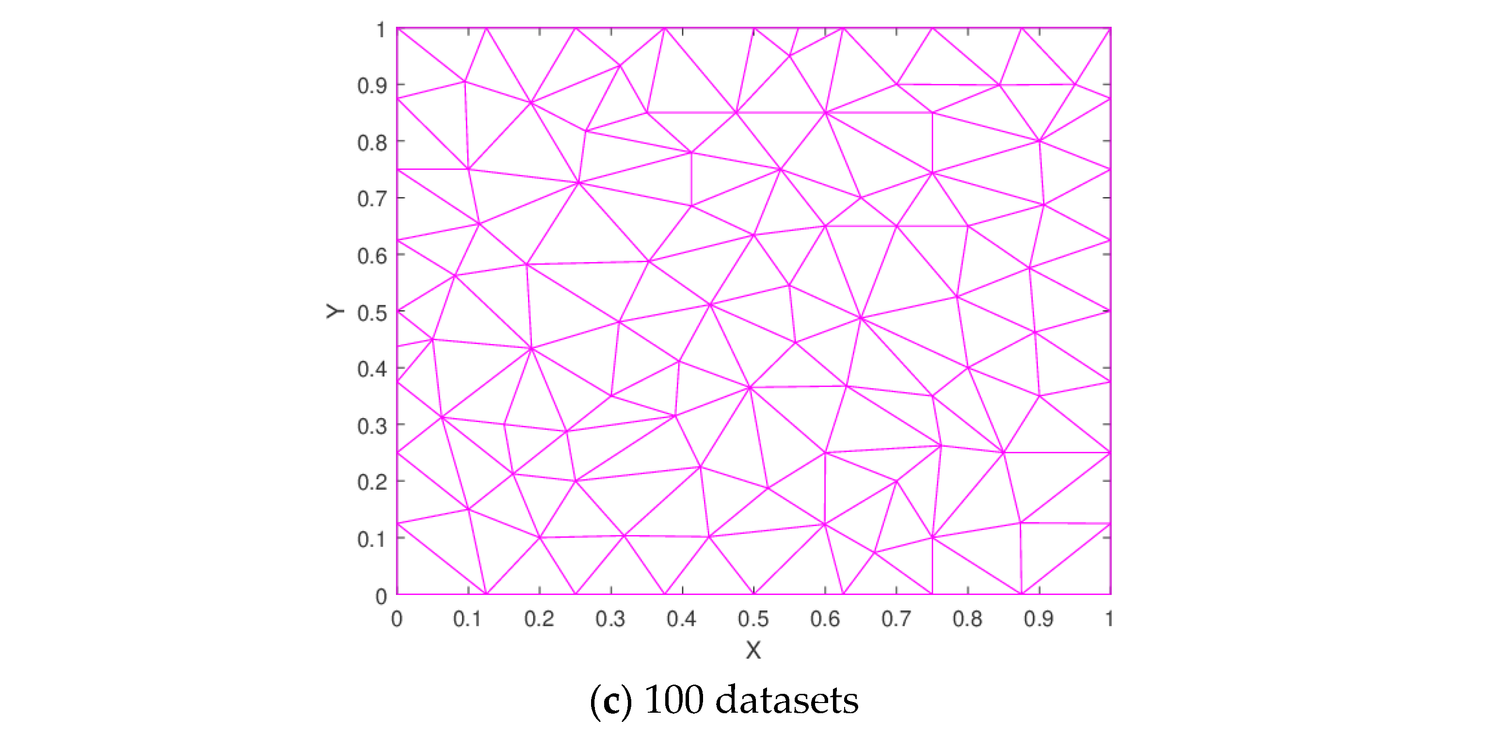
Figure 8.
Delaunay triangulation.
Figure 8.
Delaunay triangulation.
Figure 9.
3D linear interpolant for 36 datasets.
Figure 9.
3D linear interpolant for 36 datasets.
Figure 10.
3D linear interpolant for 65 datasets.
Figure 10.
3D linear interpolant for 65 datasets.
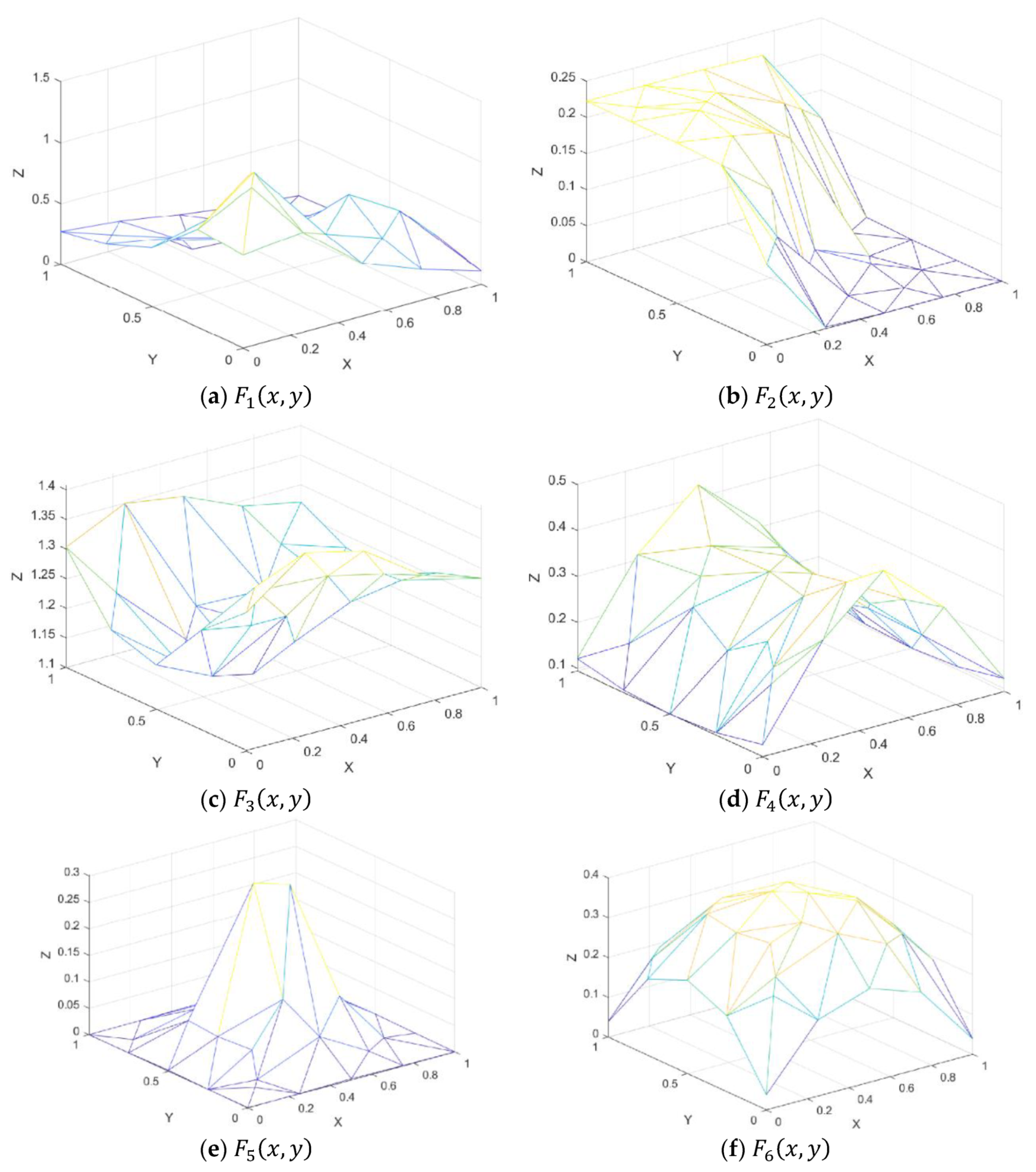
Figure 11.
3D linear interpolant for 100 datasets.
Figure 11.
3D linear interpolant for 100 datasets.
Figure 12.
Surface interpolation using Goodman and Said method and Choice 1 for 36 datasets.
Figure 12.
Surface interpolation using Goodman and Said method and Choice 1 for 36 datasets.
Figure 13.
Surface interpolation using Goodman and Said method and Choice 2 for 36 datasets.
Figure 13.
Surface interpolation using Goodman and Said method and Choice 2 for 36 datasets.
Figure 14.
Surface interpolation using Foley and Opitz method and Choice 1 for 36 datasets.
Figure 14.
Surface interpolation using Foley and Opitz method and Choice 1 for 36 datasets.
Figure 15.
Surface interpolation using Foley and Opitz method and Choice 2 for 36 datasets.
Figure 15.
Surface interpolation using Foley and Opitz method and Choice 2 for 36 datasets.
Figure 16.
Surface interpolation using Goodman and Said method and Choice 1 for 65 datasets.
Figure 16.
Surface interpolation using Goodman and Said method and Choice 1 for 65 datasets.
Figure 17.
Surface interpolation using Goodman and Said method and Choice 2 for 65 datasets.
Figure 17.
Surface interpolation using Goodman and Said method and Choice 2 for 65 datasets.
Figure 18.
Surface interpolation using Foley and Opitz method and Choice 1 for 65 datasets.
Figure 18.
Surface interpolation using Foley and Opitz method and Choice 1 for 65 datasets.
Figure 19.
Surface interpolation using Foley and Opitz method and Choice 2 for 65 datasets.
Figure 19.
Surface interpolation using Foley and Opitz method and Choice 2 for 65 datasets.
Figure 20.
Surface interpolation using Goodman and Said method and Choice 1 for 100 datasets.
Figure 20.
Surface interpolation using Goodman and Said method and Choice 1 for 100 datasets.
Figure 21.
Surface interpolation using Goodman and Said method and Choice 2 for 100 datasets.
Figure 21.
Surface interpolation using Goodman and Said method and Choice 2 for 100 datasets.
Figure 22.
Surface interpolation using Foley and Opitz method and Choice 1 for 100 datasets.
Figure 22.
Surface interpolation using Foley and Opitz method and Choice 1 for 100 datasets.
Figure 23.
Surface interpolation using Foley and Opitz method and Choice 2 for 100 datasets.
Figure 23.
Surface interpolation using Foley and Opitz method and Choice 2 for 100 datasets.
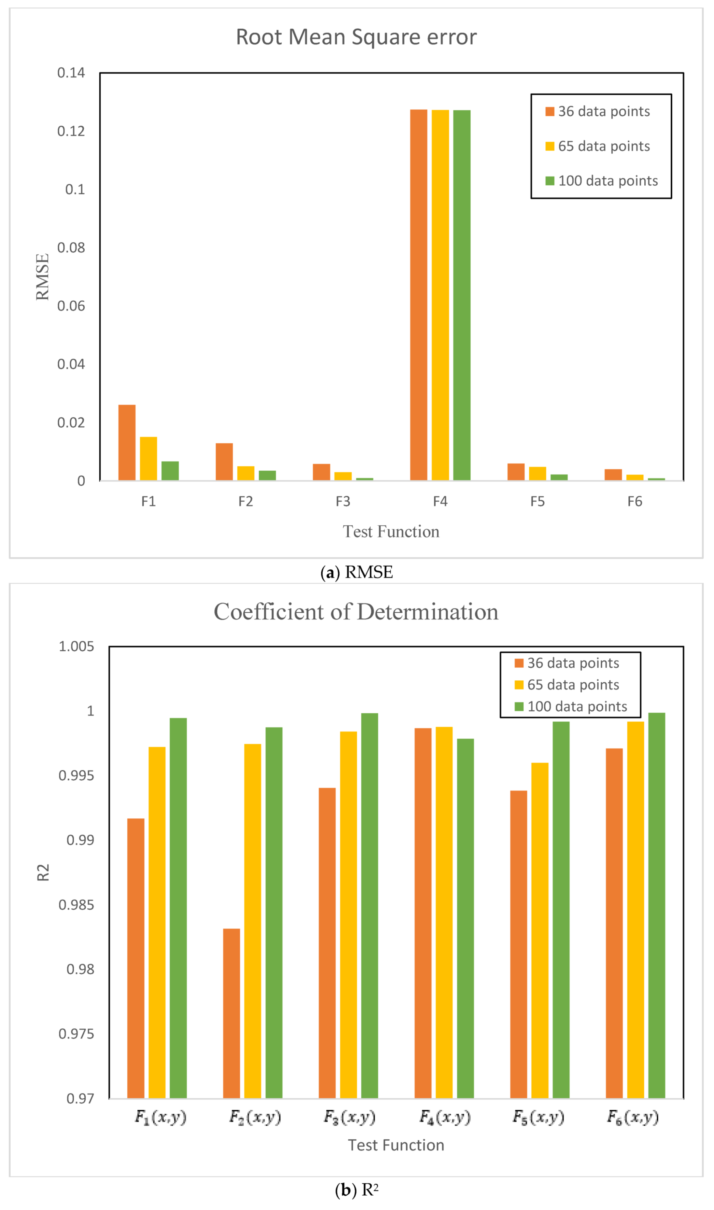
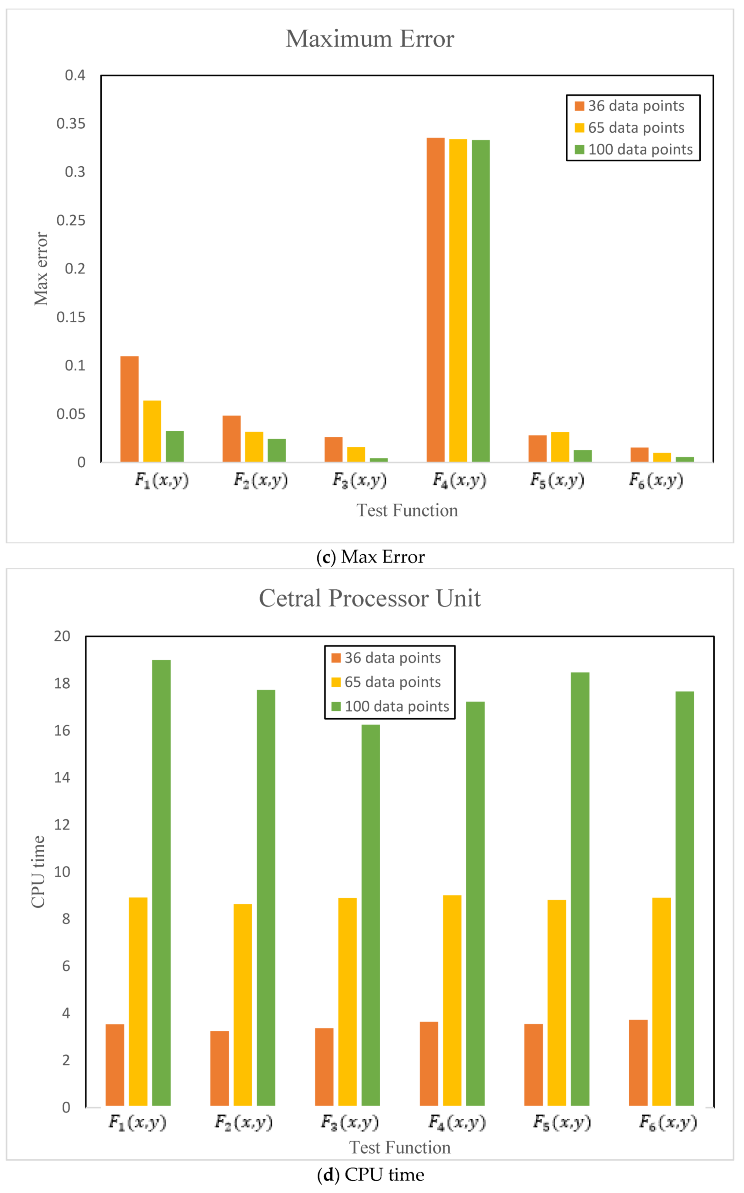
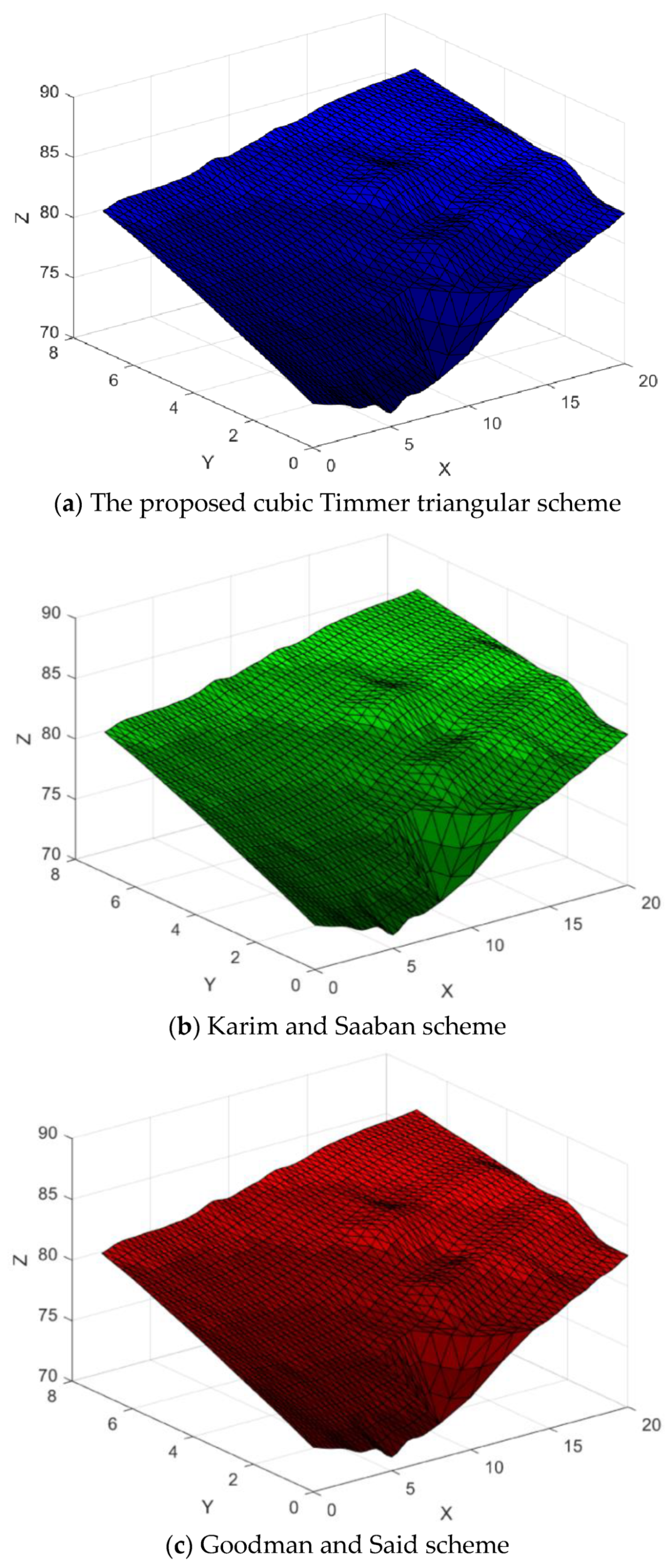
Figure 24.
Comparison of the proposed method using the best schemes.
Figure 24.
Comparison of the proposed method using the best schemes.
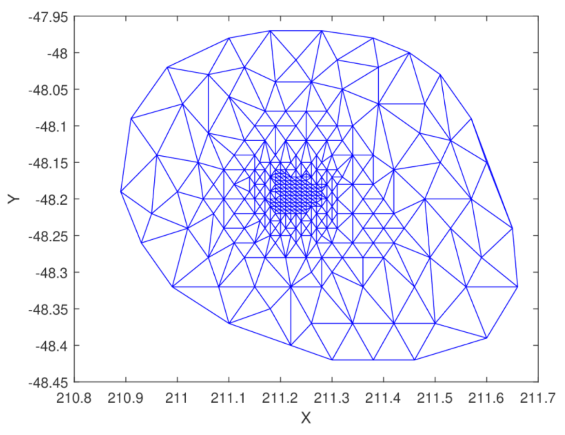
Figure 25.
Delaunay triangulation of seamount dataset.
Figure 25.
Delaunay triangulation of seamount dataset.
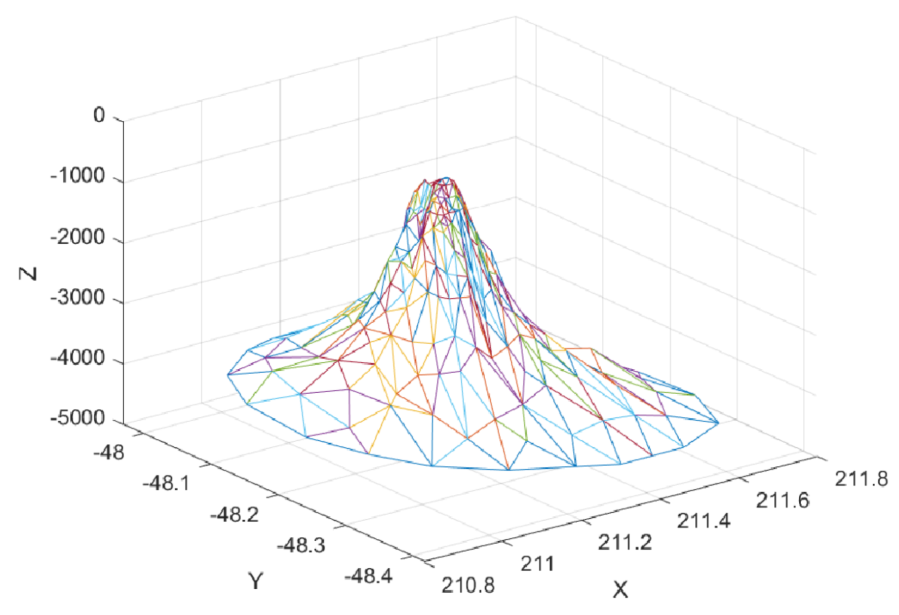
Figure 26.
3D visualization of seamount dataset.
Figure 26.
3D visualization of seamount dataset.
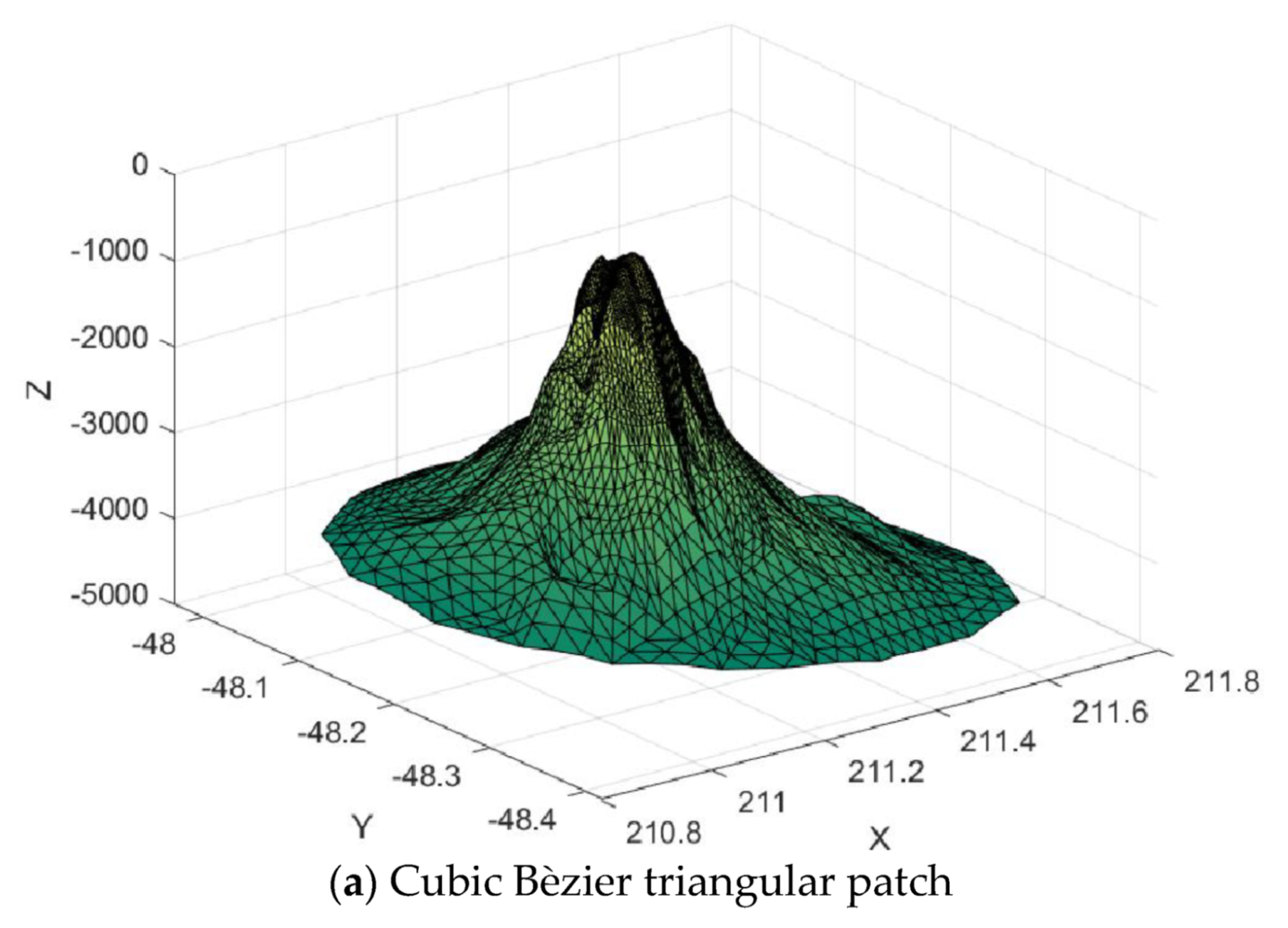
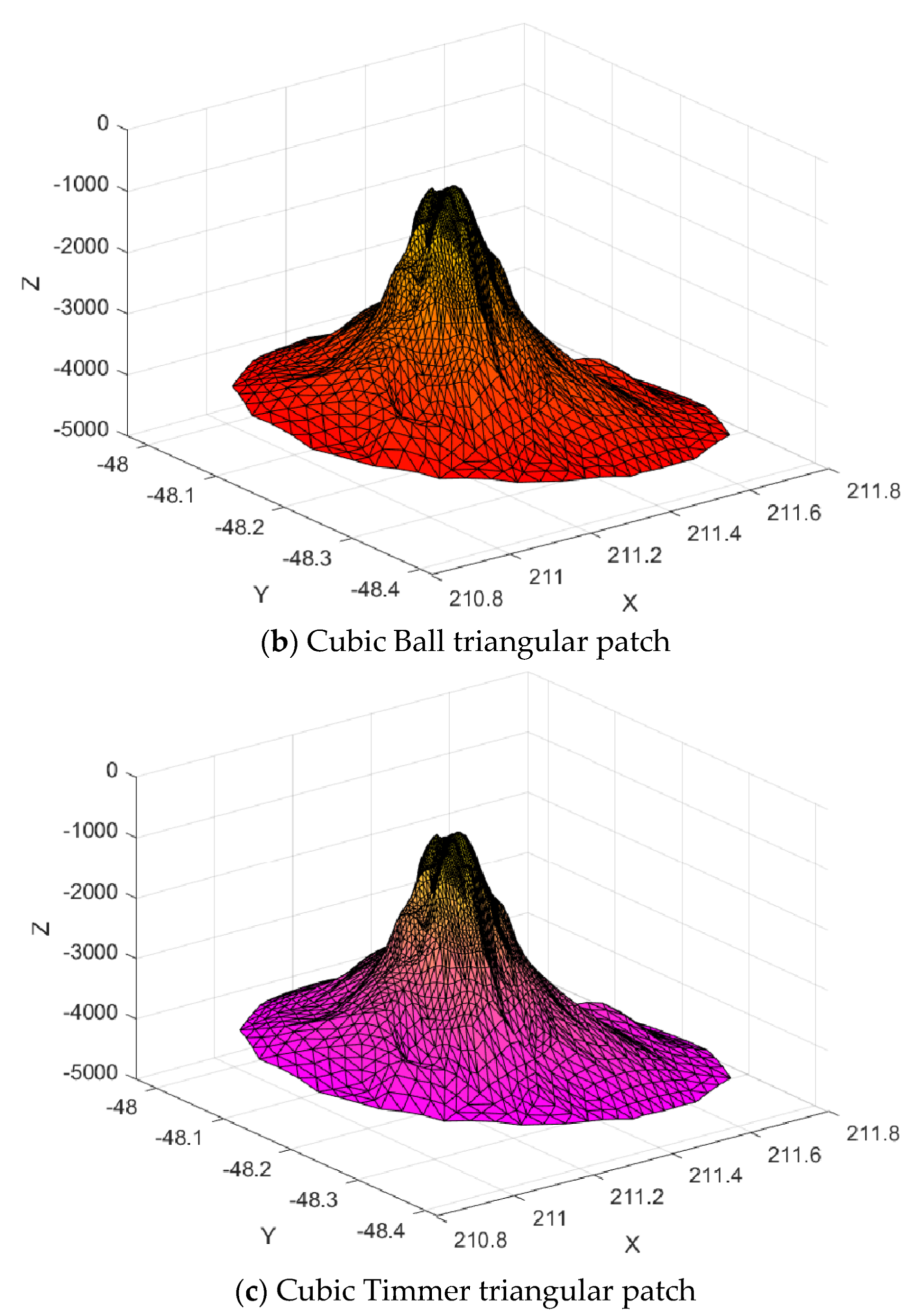
Figure 27.
Surface interpolation.
Figure 27.
Surface interpolation.
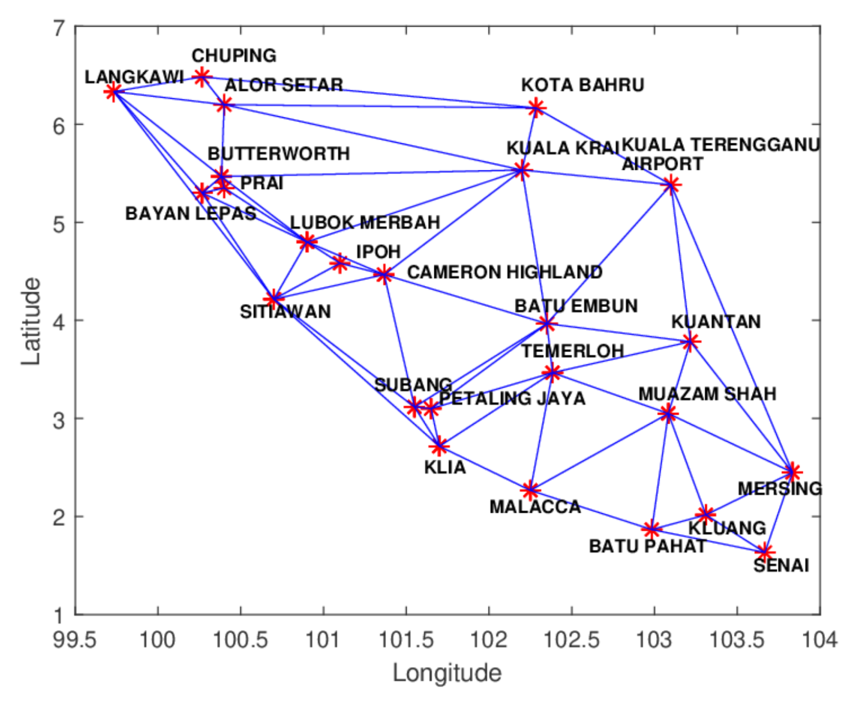
Figure 28.
Delaunay triangulation of rainfall data.
Figure 28.
Delaunay triangulation of rainfall data.
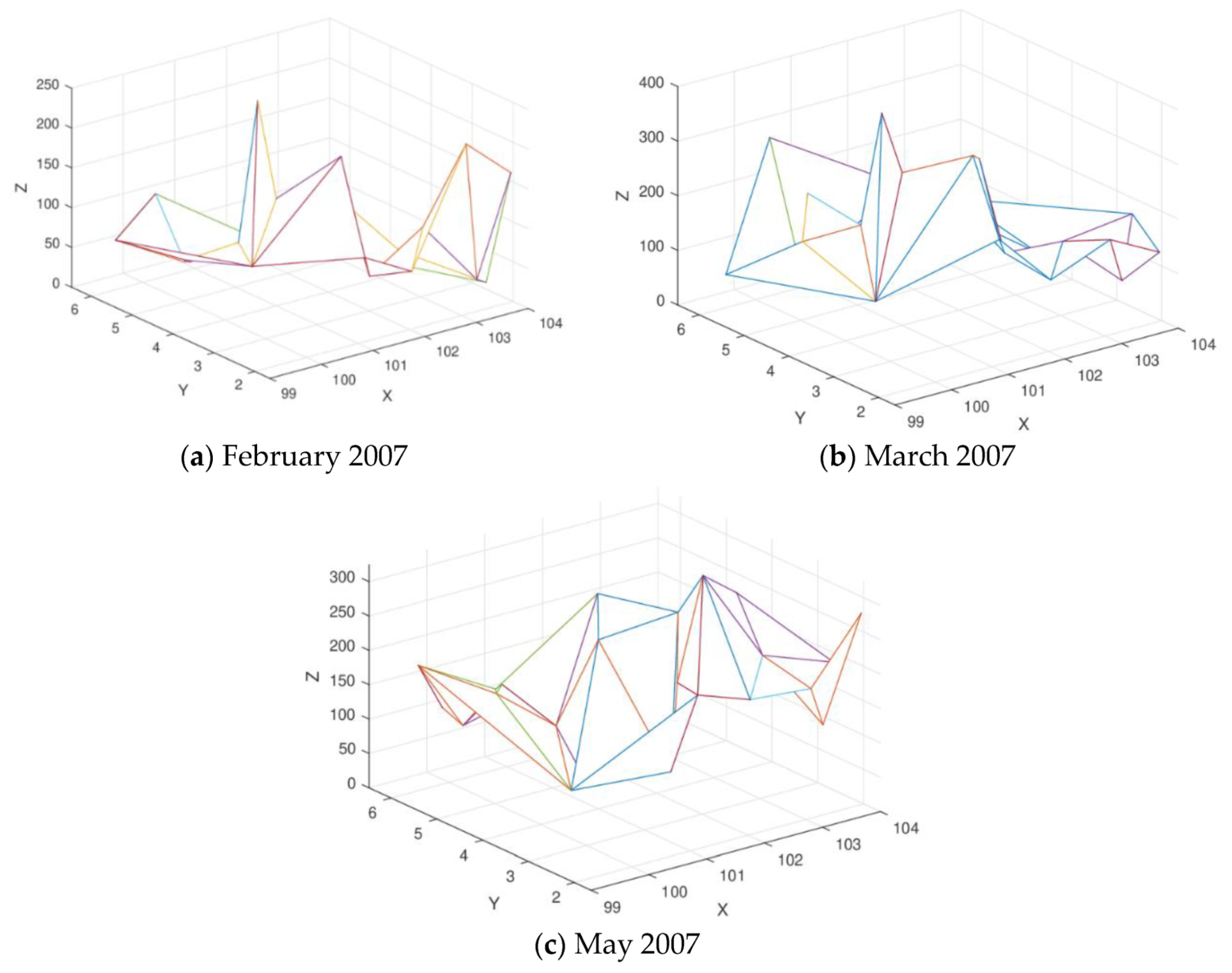
Figure 29.
3D Linear Interpolant of the rainfall data.
Figure 29.
3D Linear Interpolant of the rainfall data.
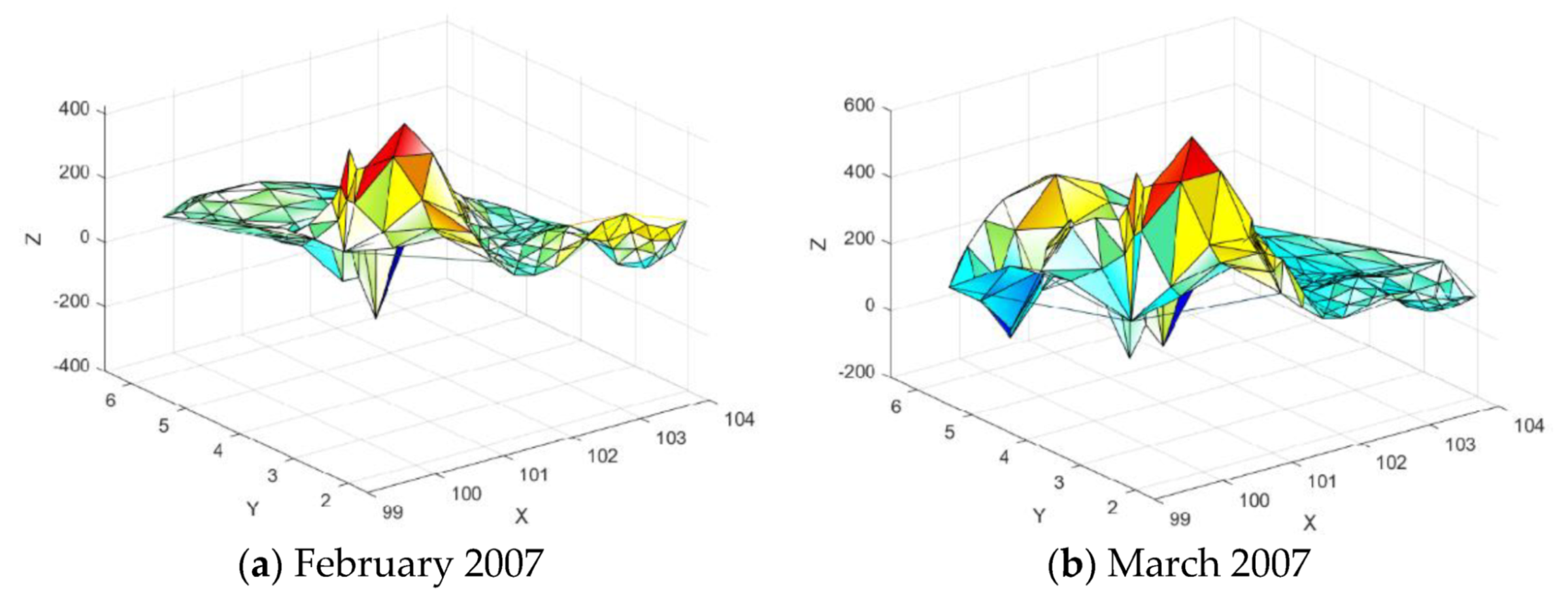
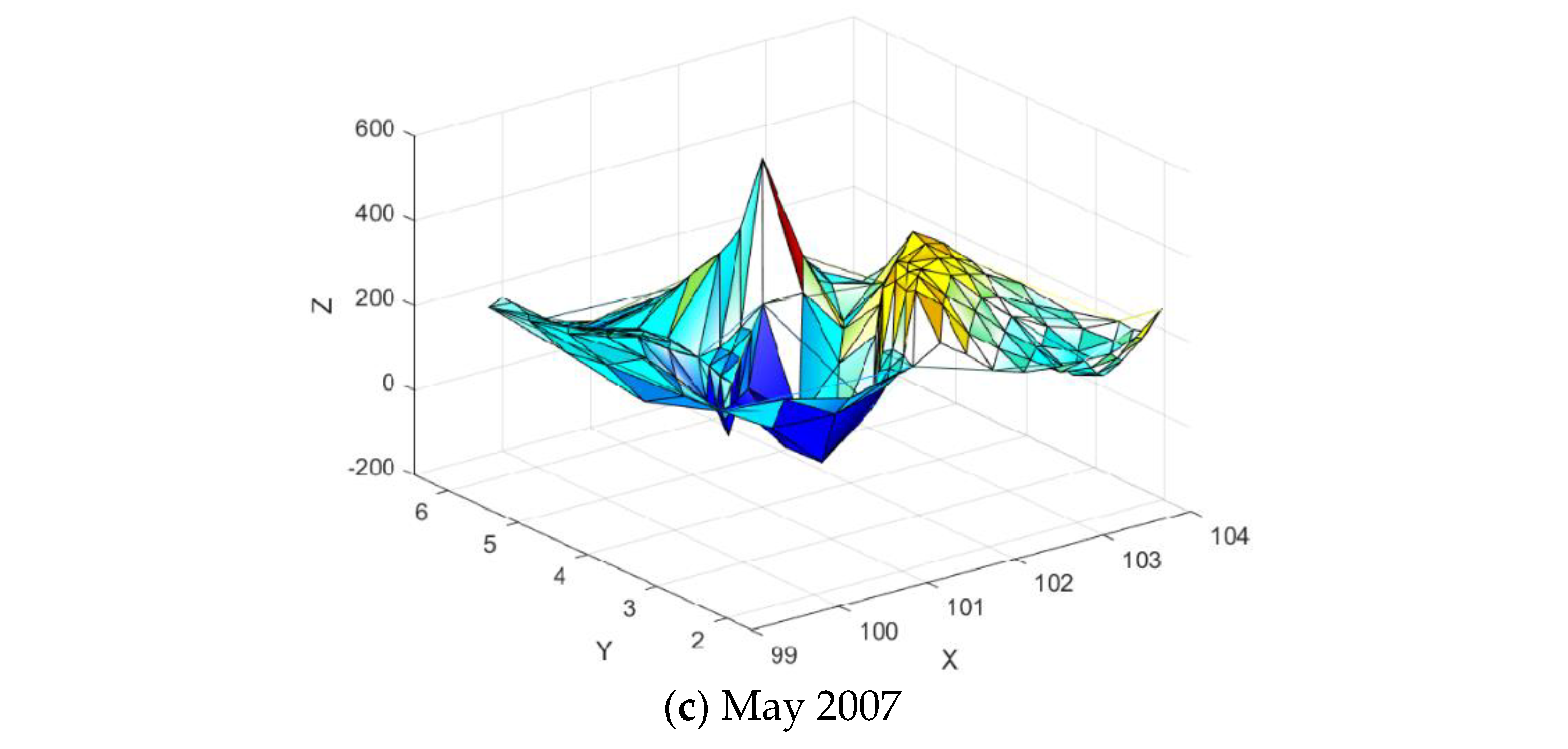
Figure 30.
Surface Interpolation using the proposed scheme.
Figure 30.
Surface Interpolation using the proposed scheme.
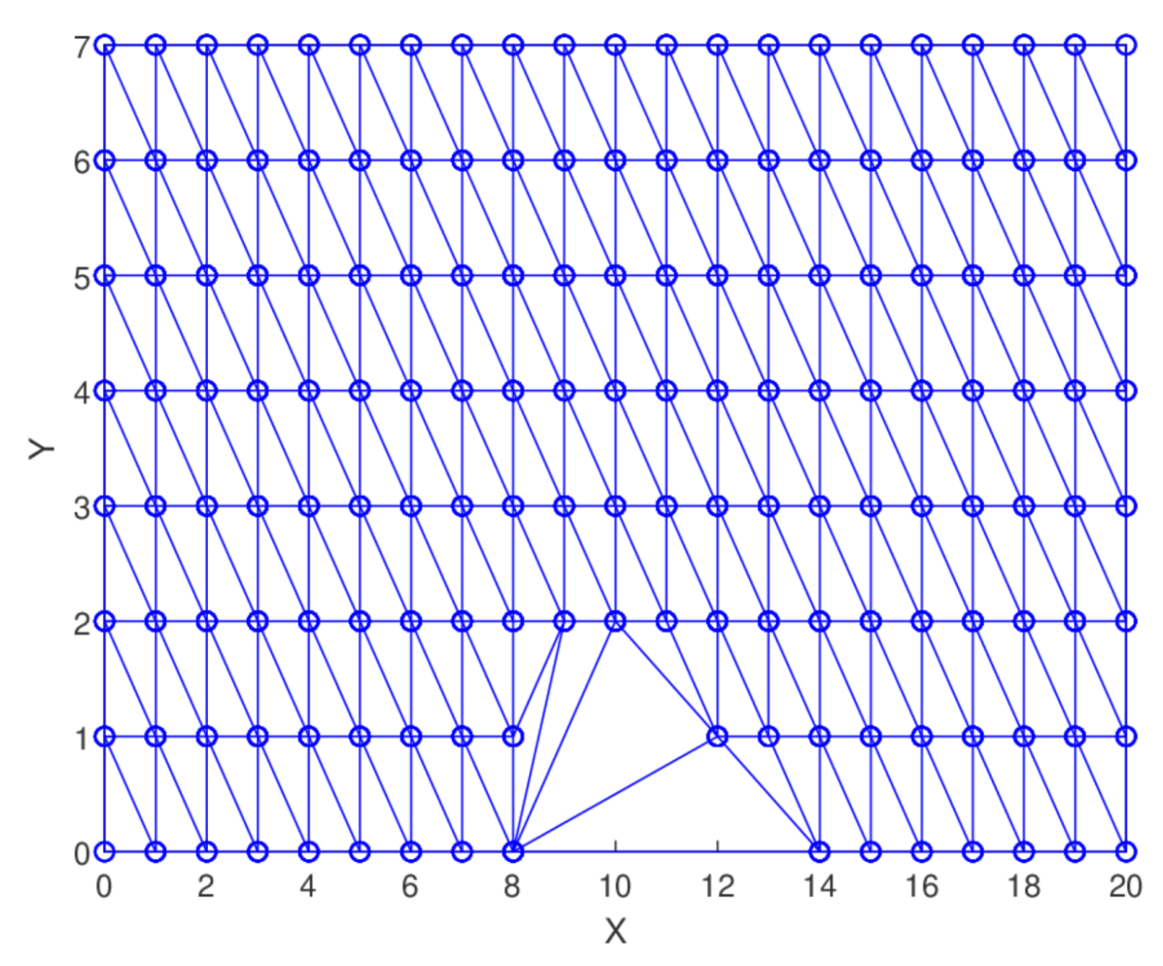
Figure 31.
Delaunay triangulation for digital elevation data.
Figure 31.
Delaunay triangulation for digital elevation data.
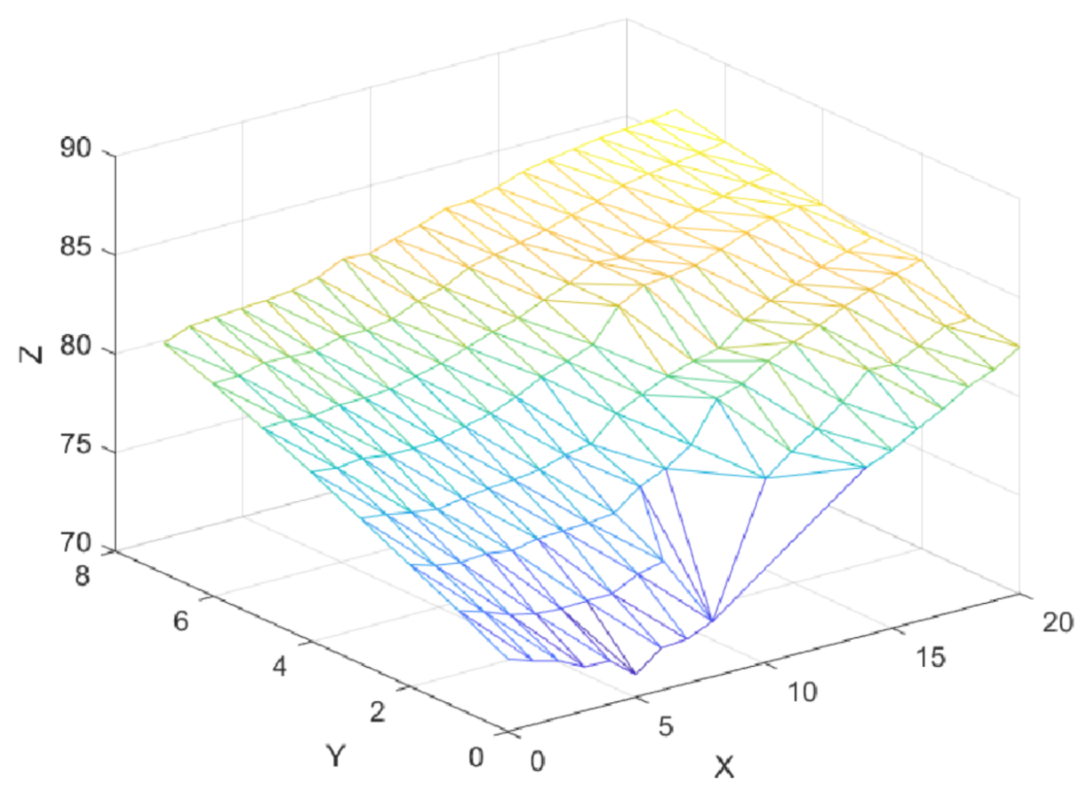
Figure 32.
3D linear interpolant for digital elevation data.
Figure 32.
3D linear interpolant for digital elevation data.
Figure 33.
Surface Interpolation.
Figure 33.
Surface Interpolation.
Table 1.
Control points.
| x | −4.0 | −4.0 | −4.0 | −4.0 | −1.5 | 1.0 | 3.5 | 1.0 | −1.5 | −1.5 |
| y | 3.5 | 1.0 | −1.5 | −4.0 | −4.0 | −4.0 | −4.0 | −1.5 | −1.5 | −1.5 |
| z | 20.25 | 9.00 | 1.0.25 | 24.00 | 10.25 | 9.00 | 20.25 | 4.75 | 4.75 | 3.50 |
Table 2.
Thirty-six datasets.
Table 2.
Thirty-six datasets.
| X | Y | | | | | | |
|---|
| 0.0000 | 0.0000 | 0.7664 | 0.1111 | 1.3333 | 0.1207 | 1.34E-05 | 0.0386 |
| 0.5000 | 0.0000 | 0.4349 | 2.74E-05 | 1.3833 | 0.4280 | 0.0021 | 0.2349 |
| 1.0000 | 0.0000 | 0.1076 | 3.38E-09 | 1.2833 | 0.1207 | 1.34E-05 | 0.0386 |
| 0.1500 | 0.1500 | 1.1370 | 0.1111 | 1.3382 | 0.2027 | 0.0023 | 0.2383 |
| 0.7000 | 0.1500 | 0.4304 | 1.11E-05 | 1.3020 | 0.3077 | 0.0124 | 0.2922 |
| 0.5000 | 0.2000 | 0.5345 | 0.0010 | 1.3128 | 0.3647 | 0.0539 | 0.3367 |
| 0.2500 | 0.3000 | 1.0726 | 0.1580 | 1.2423 | 0.2528 | 0.0418 | 0.3292 |
| 0.4000 | 0.3000 | 0.7134 | 0.0315 | 1.2421 | 0.3298 | 0.1211 | 0.3603 |
| 0.7500 | 0.4000 | 0.5903 | 0.0004 | 1.2139 | 0.2454 | 0.0768 | 0.3471 |
| 0.8500 | 0.2500 | 0.5088 | 4.53E-06 | 1.2607 | 0.1908 | 0.0079 | 0.2779 |
| 0.5500 | 0.4500 | 0.3823 | 0.0315 | 1.1613 | 0.3300 | 0.3012 | 0.3861 |
| 0.0000 | 0.5000 | 0.4818 | 0.2222 | 1.1747 | 0.0940 | 0.0021 | 0.2349 |
| 0.2000 | 0.4500 | 0.6458 | 0.2198 | 1.1412 | 0.2119 | 0.0512 | 0.3352 |
| 0.4500 | 0.5500 | 0.2946 | 0.1907 | 1.1037 | 0.3300 | 0.3012 | 0.3861 |
| 0.6000 | 0.6500 | 0.1920 | 0.1580 | 1.1552 | 0.3241 | 0.1726 | 0.3704 |
| 0.2500 | 0.7000 | 0.2930 | 0.2222 | 1.1240 | 0.2528 | 0.0418 | 0.3292 |
| 0.4000 | 0.8000 | 0.0515 | 0.2221 | 1.1887 | 0.3467 | 0.0440 | 0.3307 |
| 0.6500 | 0.7500 | 0.1372 | 0.1907 | 1.1961 | 0.3166 | 0.0596 | 0.3397 |
| 0.8000 | 0.8500 | 0.0823 | 0.1580 | 1.2431 | 0.2389 | 0.0045 | 0.2600 |
| 0.8500 | 0.6500 | 0.1412 | 0.0059 | 1.2043 | 0.1834 | 0.0177 | 0.3032 |
| 1.0000 | 0.5000 | 0.1610 | 2.74E-05 | 1.2199 | 0.0940 | 0.0021 | 0.2349 |
| 1.0000 | 1.0000 | 0.0359 | 0.1111 | 1.2712 | 0.1207 | 1.34E-05 | 0.0386 |
| 0.5000 | 1.0000 | 0.1460 | 0.2222 | 1.3346 | 0.4280 | 0.0021 | 0.2349 |
| 0.1000 | 0.8500 | 0.2935 | 0.2222 | 1.2363 | 0.1676 | 0.0011 | 0.2125 |
| 0.0000 | 1.0000 | 0.2703 | 0.2222 | 1.3029 | 0.1207 | 1.34E-05 | 0.0386 |
| 0.2500 | 0.0000 | 0.8189 | 0.0024 | 1.4069 | 0.3119 | 0.0006 | 0.1911 |
| 0.7500 | 0.0000 | 0.2521 | 3.05E-07 | 1.3150 | 0.3119 | 0.0006 | 0.1911 |
| 0.2500 | 1.0000 | 0.2222 | 0.2222 | 1.3496 | 0.3119 | 0.0006 | 0.1911 |
| 0.0000 | 0.2500 | 0.8026 | 0.2198 | 1.2683 | 0.1001 | 0.0006 | 0.1911 |
| 0.7500 | 1.0000 | 0.0810 | 0.2198 | 1.2913 | 0.3119 | 0.0006 | 0.1911 |
| 0.0000 | 0.7500 | 0.3395 | 0.2222 | 1.1987 | 0.1001 | 0.0006 | 0.1911 |
| 1.0000 | 0.2500 | 0.2302 | 3.05E-07 | 1.2573 | 0.1001 | 0.0006 | 0.1911 |
| 1.0000 | 0.7500 | 0.0504 | 0.0024 | 1.2295 | 0.1001 | 0.0006 | 0.1911 |
| 0.1900 | 0.1900 | 1.2118 | 0.1111 | 1.3229 | 0.2256 | 0.0068 | 0.2733 |
| 0.3200 | 0.7500 | 0.2029 | 0.2221 | 1.1477 | 0.3012 | 0.0488 | 0.3338 |
| 0.7900 | 0.4600 | 0.4777 | 0.0006 | 1.2041 | 0.2181 | 0.0588 | 0.3393 |
Table 3.
Sixty-five datasets.
Table 3.
Sixty-five datasets.
| X | Y | | | | | | |
|---|
| 0.0500 | 0.4500 | 0.5775 | 0.0024 | 1.1767 | 0.3119 | 0.0052 | 0.2649 |
| 0.0000 | 0.5000 | 0.4818 | 3.05E-07 | 1.1747 | 0.3119 | 0.0021 | 0.2349 |
| 0.0000 | 1.0000 | 0.2703 | 3.05E-07 | 1.3029 | 0.1001 | 1.34E-05 | 0.0386 |
| 0.0000 | 0.0000 | 0.7664 | 0.0024 | 1.3333 | 0.1001 | 1.34E-05 | 0.0386 |
| 0.1000 | 0.1500 | 1.0495 | 0.2198 | 1.3271 | 0.3119 | 0.0011 | 0.2125 |
| 0.1000 | 0.7500 | 0.3229 | 0.2222 | 1.1812 | 0.3119 | 0.0037 | 0.2534 |
| 0.1500 | 0.3000 | 1.0600 | 0.2222 | 1.2437 | 0.1001 | 0.0124 | 0.2922 |
| 0.2000 | 0.1000 | 1.0774 | 0.2198 | 1.3732 | 0.1001 | 0.0021 | 0.2349 |
| 0.2500 | 0.2000 | 1.1892 | 0.2010 | 1.3239 | 0.2100 | 0.0152 | 0.2985 |
| 0.3000 | 0.3500 | 0.8562 | 2.89E-06 | 1.1982 | 0.0955 | 0.0940 | 0.3530 |
| 0.3500 | 0.8500 | 0.1588 | 0.0212 | 1.2297 | 0.1082 | 0.0177 | 0.3032 |
| 0.5000 | 0.0000 | 0.4349 | 0.2220 | 1.3833 | 0.3955 | 0.0021 | 0.2349 |
| 0.5000 | 1.0000 | 0.1460 | 0.2220 | 1.3346 | 0.0955 | 0.0021 | 0.2349 |
| 0.5500 | 0.9500 | 0.1329 | 0.2010 | 1.2975 | 0.1082 | 0.0052 | 0.2649 |
| 0.2500 | 0.0000 | 0.8189 | 0.0004 | 1.4069 | 0.3373 | 0.0006 | 0.1911 |
| 0.7500 | 0.0000 | 0.2521 | 0.1580 | 1.3150 | 0.3241 | 0.0006 | 0.1911 |
| 1.0000 | 0.2500 | 0.2302 | 0.2198 | 1.2573 | 0.3582 | 0.0006 | 0.1911 |
| 1.0000 | 0.7500 | 0.0504 | 0.1580 | 1.2295 | 0.3096 | 0.0006 | 0.1911 |
| 0.7500 | 1.0000 | 0.0810 | 2.74E-05 | 1.2913 | 0.2979 | 0.0006 | 0.1911 |
| 0.2500 | 1.0000 | 0.2222 | 0.0642 | 1.3496 | 0.2784 | 0.0006 | 0.1911 |
| 0.0000 | 0.7500 | 0.3395 | 0.2163 | 1.1987 | 0.3195 | 0.0006 | 0.1911 |
| 0.0000 | 0.2500 | 0.8026 | 1.84E-06 | 1.2683 | 0.2851 | 0.0006 | 0.1911 |
| 0.8750 | 1.0000 | 0.0553 | 0.0002 | 1.2791 | 0.2484 | 0.0001 | 0.1321 |
| 1.0000 | 0.3750 | 0.2405 | 0.1907 | 1.2354 | 0.2746 | 0.0015 | 0.2242 |
| 1.0000 | 0.8750 | 0.0406 | 0.0002 | 1.2504 | 0.2135 | 0.0001 | 0.1321 |
| 0.6250 | 1.0000 | 0.1124 | 0.0140 | 1.3099 | 0.2162 | 0.0015 | 0.2242 |
| 0.0000 | 0.3750 | 0.6464 | 4.53E-06 | 1.2134 | 0.1908 | 0.0015 | 0.2242 |
| 0.0000 | 0.1250 | 0.8220 | 1.11E-05 | 1.3151 | 0.1517 | 0.0001 | 0.1321 |
| 0.6000 | 0.2500 | 0.5050 | 0.0315 | 1.2723 | 0.1623 | 0.0768 | 0.3471 |
| 0.6000 | 0.6500 | 0.1920 | 0.0642 | 1.1552 | 0.1403 | 0.1726 | 0.3704 |
| 0.6000 | 0.8500 | 0.1196 | 3.38E-09 | 1.2376 | 0.1207 | 0.0228 | 0.3109 |
| 0.6500 | 0.7000 | 0.1585 | 2.74E-05 | 1.1796 | 0.0940 | 0.0940 | 0.3530 |
| 0.7000 | 0.2000 | 0.5070 | 0.1111 | 1.2855 | 0.1207 | 0.0240 | 0.3125 |
| 0.7000 | 0.6500 | 0.1854 | 0.2221 | 1.1796 | 0.4196 | 0.0940 | 0.3530 |
| 0.7000 | 0.9000 | 0.1021 | 0.2221 | 1.2611 | 0.0944 | 0.0058 | 0.2682 |
| 0.7500 | 0.1000 | 0.3475 | 0.0059 | 1.3058 | 0.3494 | 0.0037 | 0.2534 |
| 0.7500 | 0.3500 | 0.6368 | 0.0212 | 1.2296 | 0.3248 | 0.0596 | 0.3397 |
| 0.7500 | 0.8500 | 0.0948 | 0.2167 | 1.2421 | 0.3091 | 0.0079 | 0.2779 |
| 0.8000 | 0.4000 | 0.5729 | 0.0457 | 1.2187 | 0.3341 | 0.0440 | 0.3307 |
| 0.8000 | 0.6500 | 0.1608 | 0.2222 | 1.1975 | 0.2414 | 0.0342 | 0.3232 |
| 0.8500 | 0.2500 | 0.5088 | 0.2221 | 1.2607 | 0.2601 | 0.0079 | 0.2779 |
| 0.9000 | 0.3500 | 0.4588 | 0.2217 | 1.2366 | 0.2132 | 0.0083 | 0.2795 |
| 0.9000 | 0.8000 | 0.0654 | 3.21E-08 | 1.2336 | 0.1082 | 0.0021 | 0.2349 |
| 0.9500 | 0.9000 | 0.0473 | 3.21E-08 | 1.2555 | 0.2100 | 0.0002 | 0.1539 |
| 1.0000 | 0.0000 | 0.1076 | 0.2207 | 1.2833 | 0.3537 | 1.34E-05 | 0.0386 |
| 1.0000 | 0.5000 | 0.1610 | 0.0005 | 1.2199 | 0.1715 | 0.0021 | 0.2349 |
| 1.0000 | 1.0000 | 0.0359 | 0.0003 | 1.2712 | 0.3955 | 1.34E-05 | 0.0386 |
| 0.5625 | 1.0000 | 0.1292 | 0.0002 | 1.3218 | 0.3797 | 0.0019 | 0.2323 |
| 0.0000 | 0.4375 | 0.5564 | 0.0061 | 1.1907 | 0.2690 | 0.0019 | 0.2323 |
| 0.4250 | 0.2250 | 0.7025 | 0.1634 | 1.3040 | 0.3345 | 0.0643 | 0.3419 |
| 0.5750 | 0.4500 | 0.3940 | 0.2222 | 1.1673 | 0.0955 | 0.2828 | 0.3843 |
| 0.3732 | 0.5768 | 0.3115 | 0.1111 | 1.0857 | 0.1207 | 0.2136 | 0.3764 |
| 0.4475 | 0.3725 | 0.5128 | 0.1111 | 1.1864 | 0.1207 | 0.2268 | 0.3781 |
| 0.2013 | 0.8592 | 0.2658 | 0.1111 | 1.2395 | 0.1207 | 0.0040 | 0.2562 |
| 0.2611 | 0.7021 | 0.2857 | 0.1111 | 1.1232 | 0.1207 | 0.0459 | 0.3320 |
| 0.2024 | 0.5368 | 0.4564 | 0.1111 | 1.1098 | 0.1207 | 0.0540 | 0.3368 |
| 1.0000 | 0.1250 | 0.1552 | 0.1111 | 1.2760 | 0.1207 | 0.0001 | 0.1321 |
| 0.8750 | 0.0000 | 0.1796 | 0.1111 | 1.2958 | 0.1207 | 0.0001 | 0.1321 |
| 0.4750 | 0.7500 | 0.0247 | 0.1111 | 1.1632 | 0.1207 | 0.0928 | 0.3526 |
| 0.8625 | 0.5250 | 0.2938 | 0.1111 | 1.2049 | 0.1207 | 0.0230 | 0.3112 |
| 0.3750 | 0.0000 | 0.6331 | 0.1111 | 1.4141 | 0.1207 | 0.0015 | 0.2242 |
| 0.5273 | 0.1341 | 0.4668 | 0.1111 | 1.3433 | 0.1207 | 0.0218 | 0.3096 |
| 0.7058 | 0.5073 | 0.3878 | 0.1111 | 1.1818 | 0.1207 | 0.1412 | 0.3647 |
| 0.5037 | 0.5605 | 0.2694 | 0.1111 | 1.1187 | 0.1207 | 0.3094 | 0.3868 |
| 0.0000 | 0.6250 | 0.3892 | 0.1111 | 1.1689 | 0.1207 | 0.0015 | 0.2242 |
Table 4.
One hundred datasets.
Table 4.
One hundred datasets.
| X | Y | | | | | | |
|---|
| 0.0500 | 0.4500 | 0.5775 | 0.2221 | 1.1767 | 0.1199 | 0.0052 | 0.2649 |
| 0.0000 | 0.5000 | 0.4818 | 0.2222 | 1.1747 | 0.0940 | 0.0021 | 0.2349 |
| 0.0000 | 1.0000 | 0.2703 | 0.2222 | 1.3029 | 0.1207 | 0.0000 | 0.0386 |
| 0.0000 | 0.0000 | 0.7664 | 0.1111 | 1.3333 | 0.1207 | 0.0000 | 0.0386 |
| 0.1000 | 0.1500 | 1.0495 | 0.1580 | 1.3271 | 0.1676 | 0.0011 | 0.2125 |
| 0.1000 | 0.7500 | 0.3229 | 0.2222 | 1.1812 | 0.1578 | 0.0037 | 0.2534 |
| 0.1500 | 0.3000 | 1.0600 | 0.2082 | 1.2437 | 0.1866 | 0.0124 | 0.2922 |
| 0.2000 | 0.1000 | 1.0774 | 0.0315 | 1.3732 | 0.2480 | 0.0021 | 0.2349 |
| 0.2500 | 0.2000 | 1.1892 | 0.0642 | 1.3239 | 0.2658 | 0.0152 | 0.2985 |
| 0.3000 | 0.3500 | 0.8562 | 0.1580 | 1.1982 | 0.2784 | 0.0940 | 0.3530 |
| 0.3500 | 0.8500 | 0.1588 | 0.2222 | 1.2297 | 0.3362 | 0.0177 | 0.3032 |
| 0.5000 | 0.0000 | 0.4349 | 0.0000 | 1.3833 | 0.4280 | 0.0021 | 0.2349 |
| 0.5000 | 1.0000 | 0.1460 | 0.2222 | 1.3346 | 0.4280 | 0.0021 | 0.2349 |
| 0.5500 | 0.9500 | 0.1329 | 0.2221 | 1.2975 | 0.4030 | 0.0052 | 0.2649 |
| 0.6000 | 0.2500 | 0.5050 | 0.0004 | 1.2723 | 0.3373 | 0.0768 | 0.3471 |
| 0.6000 | 0.6500 | 0.1920 | 0.1580 | 1.1552 | 0.3241 | 0.1726 | 0.3704 |
| 0.6000 | 0.8500 | 0.1196 | 0.2198 | 1.2376 | 0.3582 | 0.0228 | 0.3109 |
| 0.6500 | 0.7000 | 0.1585 | 0.1580 | 1.1796 | 0.3096 | 0.0940 | 0.3530 |
| 0.7000 | 0.2000 | 0.5070 | 0.0000 | 1.2855 | 0.2979 | 0.0240 | 0.3125 |
| 0.7000 | 0.6500 | 0.1854 | 0.0642 | 1.1796 | 0.2784 | 0.0940 | 0.3530 |
| 0.7000 | 0.9000 | 0.1021 | 0.2163 | 1.2611 | 0.3195 | 0.0058 | 0.2682 |
| 0.7500 | 0.1000 | 0.3475 | 0.0000 | 1.3058 | 0.2851 | 0.0037 | 0.2534 |
| 0.7500 | 0.3500 | 0.6368 | 0.0002 | 1.2296 | 0.2484 | 0.0596 | 0.3397 |
| 0.7500 | 0.8500 | 0.0948 | 0.1907 | 1.2421 | 0.2746 | 0.0079 | 0.2779 |
| 0.8000 | 0.4000 | 0.5729 | 0.0002 | 1.2187 | 0.2135 | 0.0440 | 0.3307 |
| 0.8000 | 0.6500 | 0.1608 | 0.0140 | 1.1975 | 0.2162 | 0.0342 | 0.3232 |
| 0.8500 | 0.2500 | 0.5088 | 0.0000 | 1.2607 | 0.1908 | 0.0079 | 0.2779 |
| 0.9000 | 0.3500 | 0.4588 | 0.0000 | 1.2366 | 0.1517 | 0.0083 | 0.2795 |
| 0.9000 | 0.8000 | 0.0654 | 0.0315 | 1.2336 | 0.1623 | 0.0021 | 0.2349 |
| 0.9500 | 0.9000 | 0.0473 | 0.0642 | 1.2555 | 0.1403 | 0.0002 | 0.1539 |
| 1.0000 | 0.0000 | 0.1076 | 0.0000 | 1.2833 | 0.1207 | 0.0000 | 0.0386 |
| 0.0000 | 0.6250 | 0.3892 | 0.2222 | 1.1689 | 0.0955 | 0.0015 | 0.2242 |
| 0.6250 | 0.0000 | 0.3203 | 0.0000 | 1.3444 | 0.3955 | 0.0015 | 0.2242 |
| 0.8750 | 0.0000 | 0.1796 | 0.0000 | 1.2958 | 0.2100 | 0.0001 | 0.1321 |
| 0.0000 | 0.8750 | 0.3026 | 0.2222 | 1.2511 | 0.1082 | 0.0001 | 0.1321 |
| 0.4386 | 0.5114 | 0.3383 | 0.1750 | 1.1093 | 0.3271 | 0.3080 | 0.3867 |
| 0.1816 | 0.5822 | 0.4015 | 0.2221 | 1.1119 | 0.2009 | 0.0373 | 0.3258 |
| 0.4250 | 0.2250 | 0.7025 | 0.0059 | 1.3040 | 0.3494 | 0.0643 | 0.3419 |
| 0.4750 | 0.8500 | 0.0579 | 0.2220 | 1.2328 | 0.3756 | 0.0275 | 0.3167 |
| 0.4125 | 0.6855 | 0.1477 | 0.2206 | 1.1163 | 0.3319 | 0.1422 | 0.3649 |
| 0.5993 | 0.1237 | 0.4060 | 0.0000 | 1.3299 | 0.3653 | 0.0155 | 0.2992 |
| 1.0000 | 0.1250 | 0.1552 | 0.0000 | 1.2760 | 0.1082 | 0.0001 | 0.1321 |
| 0.1250 | 1.0000 | 0.2516 | 0.2222 | 1.3261 | 0.2100 | 0.0001 | 0.1321 |
| 0.1875 | 0.8675 | 0.2679 | 0.2222 | 1.2461 | 0.2327 | 0.0030 | 0.2466 |
| 0.1250 | 0.0000 | 0.8467 | 0.0212 | 1.3699 | 0.2100 | 0.0001 | 0.1321 |
| 0.7500 | 0.7438 | 0.1181 | 0.1049 | 1.2083 | 0.2578 | 0.0282 | 0.3174 |
| 0.2545 | 0.7263 | 0.2787 | 0.2222 | 1.1378 | 0.2586 | 0.0349 | 0.3238 |
| 0.8938 | 0.4625 | 0.3559 | 0.0001 | 1.2152 | 0.1522 | 0.0140 | 0.2960 |
| 1.0000 | 0.6250 | 0.0831 | 0.0003 | 1.2176 | 0.0955 | 0.0015 | 0.2242 |
| 0.7844 | 0.5250 | 0.3500 | 0.0021 | 1.1939 | 0.2215 | 0.0640 | 0.3418 |
| 0.9063 | 0.6875 | 0.0943 | 0.0042 | 1.2145 | 0.1497 | 0.0058 | 0.2680 |
| 0.8859 | 0.5758 | 0.1981 | 0.0008 | 1.2056 | 0.1577 | 0.0145 | 0.2972 |
| 0.5375 | 0.7500 | 0.0842 | 0.2175 | 1.1755 | 0.3523 | 0.0914 | 0.3522 |
| 0.1886 | 0.4341 | 0.6915 | 0.2196 | 1.1520 | 0.2049 | 0.0428 | 0.3299 |
| 0.3112 | 0.4806 | 0.4971 | 0.2122 | 1.1082 | 0.2784 | 0.1607 | 0.3684 |
| 0.4943 | 0.3652 | 0.4735 | 0.0198 | 1.1972 | 0.3394 | 0.2306 | 0.3786 |
| 0.3528 | 0.5875 | 0.3139 | 0.2190 | 1.0840 | 0.3010 | 0.1841 | 0.3722 |
| 0.3750 | 1.0000 | 0.1842 | 0.2222 | 1.3542 | 0.3955 | 0.0015 | 0.2242 |
| 0.3125 | 0.9333 | 0.2109 | 0.2222 | 1.3034 | 0.3366 | 0.0037 | 0.2531 |
| 0.8441 | 0.8987 | 0.0676 | 0.1617 | 1.2570 | 0.2146 | 0.0012 | 0.2161 |
| 0.3954 | 0.4113 | 0.5277 | 0.1269 | 1.1525 | 0.3179 | 0.2278 | 0.3782 |
| 0.3899 | 0.3149 | 0.7178 | 0.0457 | 1.2291 | 0.3244 | 0.1303 | 0.3624 |
| 1.0000 | 0.5000 | 0.1610 | 0.0000 | 1.2199 | 0.0940 | 0.0021 | 0.2349 |
| 1.0000 | 1.0000 | 0.0359 | 0.1111 | 1.2712 | 0.1207 | 0.0000 | 0.0386 |
| 0.2500 | 0.0000 | 0.8189 | 0.0024 | 1.4069 | 0.3119 | 0.0006 | 0.1911 |
| 0.7500 | 0.0000 | 0.2521 | 0.0000 | 1.3150 | 0.3119 | 0.0006 | 0.1911 |
| 1.0000 | 0.2500 | 0.2302 | 0.0000 | 1.2573 | 0.1001 | 0.0006 | 0.1911 |
| 1.0000 | 0.7500 | 0.0504 | 0.0024 | 1.2295 | 0.1001 | 0.0006 | 0.1911 |
| 0.7500 | 1.0000 | 0.0810 | 0.2198 | 1.2913 | 0.3119 | 0.0006 | 0.1911 |
| 0.2500 | 1.0000 | 0.2222 | 0.2222 | 1.3496 | 0.3119 | 0.0006 | 0.1911 |
| 0.0000 | 0.7500 | 0.3395 | 0.2222 | 1.1987 | 0.1001 | 0.0006 | 0.1911 |
| 0.0000 | 0.2500 | 0.8026 | 0.2198 | 1.2683 | 0.1001 | 0.0006 | 0.1911 |
| 0.8750 | 1.0000 | 0.0553 | 0.2010 | 1.2791 | 0.2100 | 0.0001 | 0.1321 |
| 1.0000 | 0.3750 | 0.2405 | 0.0000 | 1.2354 | 0.0955 | 0.0015 | 0.2242 |
| 1.0000 | 0.8750 | 0.0406 | 0.0212 | 1.2504 | 0.1082 | 0.0001 | 0.1321 |
| 0.6250 | 1.0000 | 0.1124 | 0.2220 | 1.3099 | 0.3955 | 0.0015 | 0.2242 |
| 0.0000 | 0.3750 | 0.6464 | 0.2220 | 1.2134 | 0.0955 | 0.0015 | 0.2242 |
| 0.0000 | 0.1250 | 0.8220 | 0.2010 | 1.3151 | 0.1082 | 0.0001 | 0.1321 |
| 0.5625 | 1.0000 | 0.1292 | 0.2221 | 1.3218 | 0.4196 | 0.0019 | 0.2323 |
| 0.0000 | 0.4375 | 0.5564 | 0.2221 | 1.1907 | 0.0944 | 0.0019 | 0.2323 |
| 0.6500 | 0.4875 | 0.3944 | 0.0113 | 1.1735 | 0.2975 | 0.2107 | 0.3761 |
| 0.0811 | 0.5625 | 0.4329 | 0.2222 | 1.1446 | 0.1376 | 0.0088 | 0.2815 |
| 0.1154 | 0.6538 | 0.3598 | 0.2222 | 1.1420 | 0.1614 | 0.0103 | 0.2865 |
| 0.3750 | 0.0000 | 0.6331 | 0.0003 | 1.4141 | 0.3955 | 0.0015 | 0.2242 |
| 0.3181 | 0.1035 | 0.9263 | 0.0046 | 1.3910 | 0.3299 | 0.0071 | 0.2745 |
| 0.5197 | 0.1873 | 0.5032 | 0.0006 | 1.3174 | 0.3669 | 0.0457 | 0.3318 |
| 0.4371 | 0.1016 | 0.6122 | 0.0005 | 1.3796 | 0.3829 | 0.0124 | 0.2921 |
| 0.1625 | 0.2125 | 1.1918 | 0.1580 | 1.3042 | 0.2034 | 0.0062 | 0.2704 |
| 0.2375 | 0.2875 | 1.1146 | 0.1580 | 1.2528 | 0.2460 | 0.0331 | 0.3222 |
| 0.0625 | 0.3125 | 0.8667 | 0.2198 | 1.2383 | 0.1310 | 0.0034 | 0.2507 |
| 0.7625 | 0.2625 | 0.6033 | 0.0000 | 1.2596 | 0.2488 | 0.0264 | 0.3154 |
| 0.6298 | 0.3677 | 0.5269 | 0.0020 | 1.2125 | 0.3115 | 0.1663 | 0.3694 |
| 0.5495 | 0.5455 | 0.2811 | 0.1071 | 1.1349 | 0.3299 | 0.3042 | 0.3863 |
| 0.4999 | 0.6340 | 0.1996 | 0.2040 | 1.1219 | 0.3394 | 0.2317 | 0.3787 |
| 0.5581 | 0.4443 | 0.3918 | 0.0254 | 1.1656 | 0.3287 | 0.2924 | 0.3852 |
| 0.4125 | 0.7796 | 0.0310 | 0.2219 | 1.1740 | 0.3467 | 0.0586 | 0.3392 |
Table 5.
Error analysis for 36 datasets.
Table 5.
Error analysis for 36 datasets.
| Test Function | Error | Goodman and Said | Foley and Opitz |
|---|
| Choice 1 | Choice 2 | Choice 1 | Choice 2 |
|---|
| RMSE | 0.025827 | 0.025901 | 0.026097 | 0.026458 |
| R2 | 0.991858 | 0.991811 | 0.991687 | 0.991455 |
| Max error | 0.109091 | 0.110443 | 0.109642 | 0.110142 |
| CPU time | 3.666885 | 3.792837 | 3.531956 | 3.612421 |
| RMSE | 0.013091 | 0.013105 | 0.012899 | 0.012970 |
| R2 | 0.982658 | 0.982620 | 0.983163 | 0.982978 |
| Max error | 0.049755 | 0.050222 | 0.048333 | 0.049466 |
| CPU time | 3.465182 | 3.581924 | 3.238475 | 3.418465 |
| RMSE | 0.006086 | 0.006097 | 0.005834 | 0.005897 |
| R2 | 0.993518 | 0.993493 | 0.994043 | 0.993914 |
| Max error | 0.026836 | 0.026923 | 0.026082 | 0.026475 |
| CPU time | 3.381397 | 3.412042 | 3.362575 | 3.381239 |
| RMSE | 0.127280 | 0.127285 | 0.127392 | 0.127379 |
| R2 | 0.999012 | 0.998742 | 0.998671 | 0.998923 |
| Max error | 0.335392 | 0.335392 | 0.335392 | 0.335392 |
| CPU time | 3.718293 | 3.819244 | 3.634124 | 3.801234 |
| RMSE | 0.006244 | 0.006326 | 0.005952 | 0.006095 |
| R2 | 0.993218 | 0.993039 | 0.993837 | 0.993539 |
| Max error | 0.030589 | 0.031475 | 0.027931 | 0.028902 |
| CPU time | 3.931621 | 4.012938 | 3.544473 | 3.712645 |
| RMSE | 0.003587 | 0.003602 | 0.003980 | 0.003995 |
| R2 | 0.997647 | 0.997628 | 0.997104 | 0.997082 |
| Max error | 0.015551 | 0.015589 | 0.015264 | 0.014997 |
| CPU time | 3.910817 | 3.912341 | 3.722930 | 3.800012 |
Table 6.
Error analysis for 65 datasets.
Table 6.
Error analysis for 65 datasets.
| Test Function | Error | Goodman and Said | Foley and Opitz |
|---|
| Choice 1 | Choice 2 | Choice 1 | Choice 2 |
|---|
| RMSE | 0.015504 | 0.015586 | 0.015090 | 0.015246 |
| R2 | 0.997066 | 0.997034 | 0.997221 | 0.997163 |
| Max error | 0.062431 | 0.063216 | 0.063829 | 0.066465 |
| CPU time | 9.012512 | 9.214511 | 8.912451 | 9.109472 |
| RMSE | 0.005162 | 0.005177 | 0.005015 | 0.005016 |
| R2 | 0.997304 | 0.997288 | 0.997457 | 0.997454 |
| Max error | 0.030704 | 0.030792 | 0.031553 | 0.031558 |
| CPU time | 8.729935 | 9.497846 | 8.623959 | 8.761479 |
| RMSE | 0.003151 | 0.003163 | 0.003018 | 0.003091 |
| R2 | 0.998263 | 0.998249 | 0.998406 | 0.998328 |
| Max error | 0.015383 | 0.015461 | 0.015825 | 0.016667 |
| CPU time | 8.910241 | 8.948517 | 8.891025 | 8.901256 |
| RMSE | 0.127247 | 0.127249 | 0.127274 | 0.127264 |
| R2 | 0.998901 | 0.998703 | 0.998767 | 0.998513 |
| Max error | 0.333987 | 0.333987 | 0.333987 | 0.333987 |
| CPU time | 9.193316 | 9.201537 | 9.001285 | 9.182451 |
| RMSE | 0.004951 | 0.004980 | 0.004800 | 0.004877 |
| R2 | 0.995737 | 0.995686 | 0.995992 | 0.995863 |
| Max error | 0.033110 | 0.033635 | 0.031342 | 0.031923 |
| CPU time | 8.901256 | 8.924514 | 8.802561 | 8.856126 |
| RMSE | 0.001953 | 0.001959 | 0.002122 | 0.002146 |
| R2 | 0.999303 | 0.999298 | 0.999177 | 0.999158 |
| Max error | 0.010602 | 0.010715 | 0.009957 | 0.009725 |
| CPU time | 8.981256 | 8.992456 | 8.900128 | 8.941588 |
Table 7.
Error analysis for 100 datasets.
Table 7.
Error analysis for 100 datasets.
| Test Function | Error | Goodman and Said | Foley and Opitz |
|---|
| Choice 1 | Choice 2 | Choice 1 | Choice 2 |
|---|
| RMSE | 0.006834 | 0.006887 | 0.006660 | 0.006804 |
| R2 | 0.999430 | 0.999421 | 0.999459 | 0.999435 |
| Max error | 0.034165 | 0.034446 | 0.032402 | 0.032503 |
| CPU time | 19.245752 | 19.157941 | 18.989466 | 19.015484 |
| RMSE | 0.003638 | 0.003644 | 0.003525 | 0.003568 |
| R2 | 0.998661 | 0.998656 | 0.998742 | 0.998712 |
| Max error | 0.023940 | 0.024076 | 0.024344 | 0.025017 |
| CPU time | 17.772122 | 17.387878 | 17.726120 | 17.609815 |
| RMSE | 0.000997 | 0.001004 | 0.000960 | 0.001022 |
| R2 | 0.999826 | 0.999824 | 0.999839 | 0.999817 |
| Max error | 0.004870 | 0.005009 | 0.004337 | 0.004622 |
| CPU time | 17.377007 | 17.801830 | 16.248355 | 16.449573 |
| RMSE | 0.127213 | 0.127209 | 0.127199 | 0.127200 |
| R2 | 0.997790 | 0.997735 | 0.997851 | 0.997732 |
| Max error | 0.334366 | 0.334387 | 0.333155 | 0.333431 |
| CPU time | 18.517801 | 17.531418 | 17.221382 | 17. 582176 |
| RMSE | 0.002273 | 0.002299 | 0.002159 | 0.002221 |
| R2 | 0.999101 | 0.999081 | 0.999189 | 0.999142 |
| Max error | 0.012672 | 0.012685 | 0.012559 | 0.012585 |
| CPU time | 19.092384 | 19.181738 | 18.463083 | 19.083249 |
| RMSE | 0.001116 | 0.001153 | 0.000867 | 0.000868 |
| R2 | 0.999772 | 0.999757 | 0.999863 | 0.999862 |
| Max error | 0.007914 | 0.007917 | 0.005458 | 0.005459 |
| CPU time | 18.521953 | 19.728907 | 17.658403 | 18.307126 |
Table 8.
Comparison with established schemes.
Table 8.
Comparison with established schemes.
| Test Function | Error | 100 Data Points |
|---|
| Goodman and Said [8] | Karim and Saaban [21] | Proposed Scheme |
|---|
| RMSE | 0.006523 | 0.006543 | 0.006660 |
| R2 | 0.999481 | 0.999477 | 0.999459 |
| Max error | 0.032346 | 0.033434 | 0.032402 |
| CPU time | 19.853309 | 19.740250 | 18.989466 |
| RMSE | 0.003486 | 0.003464 | 0.003525 |
| R2 | 0.998770 | 0.998786 | 0.998742 |
| Max error | 0.023774 | 0.022634 | 0.024344 |
| CPU time | 18.454829 | 17.937833 | 17.726120 |
| RMSE | 0.000953 | 0.001151 | 0.000960 |
| R2 | 0.999841 | 0.999768 | 0.999839 |
| Max error | 0.004293 | 0.005725 | 0.004337 |
| CPU time | 16.947552 | 16.851681 | 16.748355 |
| RMSE | 0.127205 | 0.127190 | 0.127200 |
| R2 | 0.997654 | 0.998057 | 0.997735 |
| Max error | 0.334366 | 0.334366 | 0.334366 |
| CPU time | 18.045273 | 17.586388 | 17.582176 |
| RMSE | 0.002093 | 0.002060 | 0.002159 |
| R2 | 0.999238 | 0.999262 | 0.999189 |
| Max error | 0.012460 | 0.012264 | 0.012559 |
| CPU time | 18.675766 | 18.590993 | 18.463083 |
| RMSE | 0.000873 | 0.000881 | 0.000867 |
| R2 | 0.999861 | 0.999858 | 0.999863 |
| Max error | 0.005458 | 0.005458 | 0.005458 |
| CPU time | 17.956438 | 17.777269 | 17.658403 |
Table 9.
Seamount dataset.
Table 9.
Seamount dataset.
| X | Y | Z | X | Y | Z | X | Y | Z |
|---|
| 211.18 | −47.97 | −4250 | 211.07 | −48.18 | −3050 | 211.19 | −48.215 | −1100 |
| 211.28 | −47.97 | −4250 | 211.11 | −48.18 | −2615 | 211.2 | −48.215 | −1000 |
| 211.1 | −47.98 | −4250 | 211.15 | −48.18 | −1850 | 211.21 | −48.215 | −975 |
| 211.38 | −47.98 | −4250 | 211.17 | −48.18 | −1730 | 211.22 | −48.215 | −925 |
| 211.45 | −48 | −4250 | 211.19 | −48.18 | −1150 | 211.23 | −48.215 | −725 |
| 211.23 | −48.01 | −3900 | 211.2 | −48.18 | −1025 | 211.24 | −48.215 | −800 |
| 211.31 | −48.01 | −3950 | 211.21 | −48.18 | −600 | 211.25 | −48.215 | −1050 |
| 210.98 | −48.02 | −4250 | 211.22 | −48.18 | −900 | 210.95 | −48.22 | −4050 |
| 211.13 | −48.02 | −3900 | 211.23 | −48.18 | −1050 | 211.07 | −48.22 | −3700 |
| 211.39 | −48.02 | −4000 | 211.24 | −48.18 | −800 | 211.11 | −48.22 | −2910 |
| 211.06 | −48.03 | −4050 | 211.25 | −48.18 | −950 | 211.15 | −48.22 | −2150 |
| 211.51 | −48.03 | −4250 | 211.26 | −48.18 | −1300 | 211.17 | −48.22 | −1750 |
| 211.19 | −48.04 | −3700 | 211.27 | −48.18 | −1370 | 211.19 | −48.22 | −1250 |
| 211.26 | −48.04 | −3730 | 211.28 | −48.18 | −1450 | 211.2 | −48.22 | −1150 |
| 211.32 | −48.05 | −3650 | 211.29 | −48.18 | −1490 | 211.21 | −48.22 | −1125 |
| 211.1 | −48.06 | −3800 | 211.31 | −48.18 | −1850 | 211.22 | −48.22 | −950 |
| 211.01 | −48.07 | −3980 | 211.34 | −48.18 | −2575 | 211.23 | −48.22 | −950 |
| 211.39 | −48.07 | −3700 | 211.38 | −48.18 | −3350 | 211.24 | −48.22 | −925 |
| 211.48 | −48.07 | −3980 | 211.19 | −48.185 | −1300 | 211.25 | −48.22 | −1125 |
| 211.17 | −48.08 | −3280 | 211.2 | −48.185 | −1050 | 211.27 | −48.22 | −1350 |
| 211.21 | −48.08 | −3100 | 211.21 | −48.185 | −650 | 211.29 | −48.22 | −1650 |
| 211.25 | −48.08 | −3140 | 211.22 | −48.185 | −770 | 211.31 | −48.22 | −1750 |
| 211.29 | −48.08 | −3250 | 211.23 | −48.185 | −750 | 211.34 | −48.22 | −2500 |
| 210.91 | −48.09 | −4250 | 211.24 | −48.185 | −620 | 211.38 | −48.22 | −3025 |
| 211.57 | −48.09 | −4250 | 211.25 | −48.185 | −950 | 211.42 | −48.22 | −3400 |
| 211.15 | −48.1 | −3150 | 211.26 | −48.185 | −1150 | 211.16 | −48.23 | −2200 |
| 211.19 | −48.1 | −3000 | 211.27 | −48.185 | −1000 | 211.18 | −48.23 | −1850 |
| 211.23 | −48.1 | −2850 | 211.28 | −48.185 | −1150 | 211.2 | −48.23 | −1500 |
| 211.27 | −48.1 | −3000 | 210.89 | −48.19 | −4250 | 211.22 | −48.23 | −1325 |
| 211.31 | −48.1 | −3100 | 211 | −48.19 | −3650 | 211.24 | −48.23 | −1375 |
| 211.34 | −48.1 | −3220 | 211.14 | −48.19 | −2300 | 211.26 | −48.23 | −1530 |
| 211.06 | −48.11 | −3630 | 211.16 | −48.19 | −1940 | 211.28 | −48.23 | −1680 |
| 211.47 | −48.11 | −3765 | 211.18 | −48.19 | −1550 | 211.3 | −48.23 | −2000 |
| 211.13 | −48.12 | −3170 | 211.2 | −48.19 | −1050 | 211.02 | −48.24 | −3700 |
| 211.17 | −48.12 | −2875 | 211.21 | −48.19 | −675 | 211.09 | −48.24 | −3325 |
| 211.21 | −48.12 | −2600 | 211.22 | −48.19 | −600 | 211.13 | −48.24 | −2875 |
| 211.25 | −48.12 | −2600 | 211.23 | −48.19 | −590 | 211.17 | −48.24 | −2200 |
| 211.29 | −48.12 | −2575 | 211.24 | −48.19 | −650 | 211.19 | −48.24 | −1850 |
| 211.32 | −48.12 | −2950 | 211.25 | −48.19 | −800 | 211.21 | −48.24 | −1600 |
| 211.53 | −48.12 | −4070 | 211.26 | −48.19 | −1050 | 211.23 | −48.24 | −1900 |
| 210.96 | −48.14 | −3920 | 211.27 | −48.19 | −950 | 211.25 | −48.24 | −1800 |
| 211.11 | −48.14 | −2950 | 211.28 | −48.19 | −1000 | 211.27 | −48.24 | −1930 |
| 211.15 | −48.14 | −2550 | 211.3 | −48.19 | −1780 | 211.29 | −48.24 | −2000 |
| 211.19 | −48.14 | −2350 | 211.19 | −48.19 | −1150 | 211.31 | −48.24 | −2250 |
| 211.23 | −48.14 | −2195 | 211.2 | −48.195 | −850 | 211.36 | −48.24 | −2800 |
| 211.27 | −48.14 | −2080 | 211.21 | −48.195 | −600 | 211.4 | −48.24 | −3220 |
| 211.3 | −48.14 | −2450 | 211.22 | −48.195 | −570 | 211.44 | −48.24 | −3500 |
| 211.34 | −48.14 | −2925 | 211.23 | −48.195 | −555 | 211.53 | −48.24 | −3650 |
| 211.38 | −48.14 | −3125 | 211.24 | −48.195 | −580 | 211.65 | −48.24 | −4250 |
| 211.04 | −48.15 | −3450 | 211.25 | −48.195 | −700 | 211.18 | −48.25 | −2150 |
| 211.16 | −48.15 | −2110 | 211.26 | −48.195 | −750 | 211.2 | −48.25 | −1840 |
| 211.18 | −48.15 | −2100 | 211.27 | −48.195 | −875 | 211.22 | −48.25 | −2275 |
| 211.2 | −48.15 | −1760 | 211.28 | −48.195 | −1020 | 211.24 | −48.25 | −2275 |
| 211.22 | −48.15 | −1920 | 211.05 | −48.2 | −3275 | 211.26 | −48.25 | −2150 |
| 211.24 | −48.15 | −1900 | 211.09 | −48.2 | −2865 | 211.28 | −48.25 | −2250 |
| 211.26 | −48.15 | −1750 | 211.13 | −48.2 | −2480 | 210.93 | −48.26 | −4250 |
| 211.28 | −48.15 | −2110 | 211.15 | −48.2 | −2025 | 211.11 | −48.26 | −3240 |
| 211.51 | −48.15 | −3950 | 211.17 | −48.2 | −1375 | 211.15 | −48.26 | −2675 |
| 211.6 | −48.15 | −4250 | 211.18 | −48.2 | −1000 | 211.19 | −48.26 | −2100 |
| 211.09 | −48.16 | −2950 | 211.19 | −48.2 | −825 | 211.23 | −48.26 | −2575 |
| 211.13 | −48.16 | −2570 | 211.2 | −48.2 | −700 | 211.27 | −48.26 | −2400 |
| 211.15 | −48.16 | −1950 | 211.21 | −48.2 | −580 | 211.3 | −48.26 | −2550 |
| 211.17 | −48.16 | −1750 | 211.22 | −48.2 | −510 | 211.34 | −48.26 | −2820 |
| 211.19 | −48.16 | −1480 | 211.23 | −48.2 | −500 | 211.38 | −48.26 | −3050 |
| 211.2 | −48.16 | −1325 | 211.24 | −48.2 | −550 | 211.42 | −48.26 | −3400 |
| 211.21 | −48.16 | −1350 | 211.25 | −48.2 | −600 | 211.06 | −48.28 | −3725 |
| 211.23 | −48.16 | −1650 | 211.26 | −48.2 | −735 | 211.13 | −48.28 | −3120 |
| 211.25 | −48.16 | −1375 | 211.27 | −48.2 | −875 | 211.17 | −48.28 | −2800 |
| 211.27 | −48.16 | −1780 | 211.28 | −48.2 | −1150 | 211.21 | −48.28 | −3050 |
| 211.29 | −48.16 | −2125 | 211.29 | −48.2 | −1500 | 211.25 | −48.28 | −2925 |
| 211.31 | −48.16 | −2200 | 211.31 | −48.2 | −2150 | 211.28 | −48.28 | −2775 |
| 211.36 | −48.16 | −2940 | 211.36 | −48.2 | −3000 | 211.32 | −48.28 | −2920 |
| 211.42 | −48.16 | −3450 | 211.4 | −48.2 | −3380 | 211.36 | −48.28 | −3190 |
| 211.19 | −48.165 | −1150 | 211.48 | −48.2 | −3780 | 211.4 | −48.28 | −3260 |
| 211.2 | −48.165 | −1125 | 211.57 | −48.2 | −4025 | 211.49 | −48.28 | −3780 |
| 211.21 | −48.165 | −1150 | 211.18 | −48.205 | −950 | 211.59 | −48.28 | −4050 |
| 211.25 | −48.165 | −1125 | 211.19 | −48.205 | −800 | 211.26 | −48.3 | −3250 |
| 211.14 | −48.17 | −2250 | 211.2 | −48.205 | −740 | 211.3 | −48.3 | −3140 |
| 211.16 | −48.17 | −1875 | 211.21 | −48.205 | −595 | 210.99 | −48.32 | −4250 |
| 211.18 | −48.17 | −1340 | 211.22 | −48.205 | −595 | 211.08 | −48.32 | −3950 |
| 211.19 | −48.17 | −1075 | 211.23 | −48.205 | −490 | 211.15 | −48.32 | −3750 |
| 211.2 | −48.17 | −850 | 211.24 | −48.205 | −650 | 211.22 | −48.32 | −3630 |
| 211.21 | −48.17 | −850 | 211.25 | −48.205 | −748 | 211.28 | −48.32 | −3420 |
| 211.22 | −48.17 | −1100 | 211.26 | −48.205 | −850 | 211.36 | −48.32 | −3420 |
| 211.23 | −48.17 | −1375 | 211.27 | −48.205 | −1000 | 211.46 | −48.32 | −3735 |
| 211.24 | −48.17 | −1175 | 211.16 | −48.21 | −1700 | 211.56 | −48.32 | −4015 |
| 211.25 | −48.17 | −950 | 211.18 | −48.21 | −1200 | 211.66 | −48.32 | −4250 |
| 211.26 | −48.17 | −1300 | 211.19 | −48.21 | −1000 | 211.18 | −48.35 | −4010 |
| 211.28 | −48.17 | −1825 | 211.2 | −48.21 | −850 | 211.1 | −48.37 | −4250 |
| 211.3 | −48.17 | −1850 | 211.21 | −48.21 | −765 | 211.26 | −48.37 | −3950 |
| 211.32 | −48.17 | −2110 | 211.22 | −48.21 | −780 | 211.34 | −48.37 | −3850 |
| 211.19 | −48.175 | −1125 | 211.23 | −48.21 | −560 | 211.42 | −48.37 | −3900 |
| 211.2 | −48.175 | −800 | 211.24 | −48.21 | −750 | 211.5 | −48.37 | −4050 |
| 211.21 | −48.175 | −700 | 211.25 | −48.21 | −850 | 211.6 | −48.39 | −4250 |
| 211.22 | −48.175 | −1020 | 211.26 | −48.21 | −1040 | 211.22 | −48.4 | −4250 |
| 211.23 | −48.175 | −1175 | 211.27 | −48.21 | −1200 | 211.3 | −48.42 | −4250 |
| 211.24 | −48.175 | −900 | 211.28 | −48.21 | −1300 | 211.38 | −48.42 | −4250 |
| 211.25 | −48.175 | −900 | 211.3 | −48.21 | −1600 | | | |
Table 10.
Rainfall data.
| Station | Location | Average Rainfall (mm) |
|---|
| Longitude | Latitude | Feb | March | May |
|---|
| Chuping | 100.2667 | 6.4833 | 68.6 | 61.0 | 88.0 |
| Langkawi Island | 99.7333 | 6.3333 | 49.8 | 40.6 | 166.0 |
| Alor Setar | 100.4000 | 6.2000 | 99.4 | 277.8 | 67.4 |
| Butterworth | 100.3833 | 5.4667 | 31.6 | 58.9 | 143.2 |
| Prai | 100.4000 | 5.3500 | 33.8 | 208.1 | 153.4 |
| Bayan Lepas | 100.2667 | 5.3000 | 39.8 | 125.2 | 144.4 |
| Ipoh | 101.1000 | 4.5833 | 242.4 | 364.2 | 42.6 |
| Cameron Highlands | 101.3667 | 4.4667 | 117.2 | 252.0 | 223.2 |
| Lubok Merbau | 100.9000 | 4.8000 | 62.6 | 156.4 | 98.4 |
| Sitiawan | 100.7000 | 4.2167 | 49.8 | 44.4 | 26.8 |
| Subang | 101.5500 | 3.1167 | 199.0 | 329.2 | 68.2 |
| Petaling Jaya | 101.6500 | 3.1000 | 139.8 | 321.0 | 196.2 |
| KLIA (Sepang) | 101.7000 | 2.7167 | 78.6 | 186.2 | 188.8 |
| Melaka | 102.2500 | 2.2667 | 62.4 | 113.8 | 183.4 |
| Batu Pahat | 102.9833 | 1.8667 | 219.0 | 182.0 | 195.0 |
| Kluang | 103.3100 | 2.0167 | 39.4 | 92.4 | 130.2 |
| Senai | 103.6667 | 1.6333 | 176.3 | 148.6 | 296.0 |
| Kota Bahru | 102.2833 | 6.1667 | 7.0 | 115.2 | 109.2 |
| Kuala Krai | 102.2000 | 5.5333 | 16.6 | 166.0 | 238.7 |
| Kuala Terengganu | 103.1000 | 5.3833 | 0.2 | 121.0 | 64.8 |
| Kuantan | 103.2167 | 3.7833 | 35.2 | 79.2 | 270.4 |
| Batu Embun | 102.3500 | 3.9667 | 103.2 | 146.2 | 256.2 |
| Temerloh | 102.3833 | 3.4667 | 25.6 | 114.2 | 324.2 |
| Muadzam Shah | 103.0833 | 3.0500 | 85.0 | 131.6 | 204.8 |
| Mersing | 103.8333 | 2.4500 | 16.4 | 183.4 | 196.2 |
Table 11.
Minimum value (mm).
Table 11.
Minimum value (mm).
| Average Rainfall (mm) | Minimum Value (mm) |
|---|
| Feb | −259.9196 |
| March | −165.0851 |
| May | −71.3284 |
Table 12.
Digital elevation data of Kalumpang Agricultural Station.
Table 12.
Digital elevation data of Kalumpang Agricultural Station.
| X | Y | Z | X | Y | Z | X | Y | Z |
|---|
| 0 | 0 | 73.70 | 6 | 6 | 81.40 | 14 | 4 | 83.60 |
| 0 | 1 | 75.00 | 6 | 7 | 82.90 | 14 | 5 | 83.40 |
| 0 | 2 | 76.20 | 7 | 0 | 72.25 | 14 | 6 | 84.40 |
| 0 | 3 | 77.40 | 7 | 1 | 74.40 | 14 | 7 | 85.45 |
| 0 | 4 | 78.60 | 7 | 2 | 75.85 | 15 | 0 | 79.00 |
| 0 | 5 | 79.70 | 7 | 3 | 77.40 | 15 | 1 | 80.30 |
| 0 | 6 | 80.80 | 7 | 4 | 79.10 | 15 | 2 | 82.20 |
| 0 | 7 | 81.70 | 7 | 5 | 80.50 | 15 | 3 | 82.20 |
| 1 | 0 | 73.25 | 7 | 6 | 81.60 | 15 | 4 | 83.80 |
| 1 | 1 | 74.60 | 7 | 7 | 83.50 | 15 | 5 | 83.90 |
| 1 | 2 | 75.80 | 8 | 0 | 72.80 | 15 | 6 | 84.75 |
| 1 | 3 | 77.25 | 8 | 1 | 74.70 | 15 | 7 | 85.70 |
| 1 | 4 | 78.45 | 8 | 2 | 76.00 | 16 | 0 | 79.75 |
| 1 | 5 | 79.70 | 8 | 3 | 77.80 | 16 | 1 | 81.60 |
| 1 | 6 | 80.85 | 8 | 4 | 79.60 | 16 | 2 | 82.70 |
| 1 | 7 | 82.20 | 8 | 5 | 80.95 | 16 | 3 | 82.80 |
| 2 | 0 | 72.90 | 8 | 6 | 82.15 | 16 | 4 | 84.25 |
| 2 | 1 | 74.10 | 8 | 7 | 83.40 | 16 | 5 | 84.25 |
| 2 | 2 | 75.60 | 9 | 2 | 77.00 | 16 | 6 | 85.20 |
| 2 | 3 | 77.00 | 9 | 3 | 78.00 | 16 | 7 | 85.90 |
| 2 | 4 | 78.60 | 9 | 4 | 80.25 | 17 | 0 | 80.40 |
| 2 | 5 | 79.60 | 9 | 5 | 81.40 | 17 | 1 | 81.50 |
| 2 | 6 | 81.15 | 9 | 6 | 82.50 | 17 | 2 | 83.30 |
| 2 | 7 | 82.30 | 9 | 7 | 83.80 | 17 | 3 | 83.30 |
| 3 | 0 | 72.25 | 10 | 2 | 77.55 | 17 | 4 | 84.75 |
| 3 | 1 | 73.80 | 10 | 3 | 79.20 | 17 | 5 | 84.75 |
| 3 | 2 | 75.70 | 10 | 4 | 80.70 | 17 | 6 | 85.45 |
| 3 | 3 | 76.80 | 10 | 5 | 81.75 | 17 | 7 | 86.10 |
| 3 | 4 | 78.40 | 10 | 6 | 83.15 | 18 | 0 | 81.20 |
| 3 | 5 | 79.80 | 10 | 7 | 84.15 | 18 | 1 | 82.10 |
| 3 | 6 | 81.10 | 11 | 2 | 78.40 | 18 | 2 | 83.80 |
| 3 | 7 | 82.40 | 11 | 3 | 79.80 | 18 | 3 | 83.80 |
| 4 | 0 | 72.20 | 11 | 4 | 81.20 | 18 | 4 | 85.15 |
| 4 | 1 | 73.70 | 11 | 5 | 82.30 | 18 | 5 | 85.10 |
| 4 | 2 | 75.50 | 11 | 6 | 83.45 | 18 | 6 | 85.60 |
| 4 | 3 | 77.00 | 11 | 7 | 84.65 | 18 | 7 | 86.20 |
| 4 | 4 | 78.40 | 12 | 1 | 77.50 | 19 | 0 | 81.70 |
| 4 | 5 | 79.80 | 12 | 2 | 80.40 | 19 | 1 | 82.75 |
| 4 | 6 | 81.05 | 12 | 3 | 80.40 | 19 | 2 | 84.25 |
| 4 | 7 | 82.45 | 12 | 4 | 82.80 | 19 | 3 | 84.25 |
| 5 | 0 | 71.15 | 12 | 5 | 82.80 | 19 | 4 | 85.40 |
| 5 | 1 | 73.75 | 12 | 6 | 83.70 | 19 | 5 | 85.40 |
| 5 | 2 | 75.75 | 12 | 7 | 84.70 | 19 | 6 | 85.80 |
| 5 | 3 | 77.15 | 13 | 1 | 78.50 | 19 | 7 | 86.30 |
| 5 | 4 | 78.50 | 13 | 2 | 80.80 | 20 | 0 | 82.50 |
| 5 | 5 | 79.90 | 13 | 3 | 80.80 | 20 | 1 | 82.80 |
| 5 | 6 | 81.40 | 13 | 4 | 83.50 | 20 | 2 | 84.60 |
| 5 | 7 | 82.60 | 13 | 5 | 83.50 | 20 | 3 | 84.60 |
| 6 | 0 | 72.15 | 13 | 6 | 84.00 | 20 | 4 | 85.10 |
| 6 | 1 | 73.75 | 13 | 7 | 85.00 | 20 | 5 | 85.60 |
| 6 | 2 | 75.80 | 14 | 0 | 78.50 | 20 | 6 | 86.00 |
| 6 | 3 | 77.25 | 14 | 1 | 79.30 | 20 | 7 | 86.50 |
| 6 | 4 | 78.80 | 14 | 2 | 81.60 | | | |
| 6 | 5 | 80.20 | 14 | 3 | 81.10 | | | |

 ,
, 


