Two-Parameter Stochastic Weibull Diffusion Model: Statistical Inference and Application to Real Modeling Example

Abstract

This paper describes the use of the non-homogeneous stochastic Weibull diffusion process, based on the two-parameter Weibull density function (the trend of which is proportional to the two-parameter Weibull probability density function). The trend function (conditioned and non-conditioned) is analyzed to obtain fits and forecasts for a real data set, taking into account the mean value of the process, the maximum likelihood estimators of the parameters of the model and the computational problems that may arise. To carry out the task, we employ the simulated annealing method for finding the estimators values and achieve the study. Finally, to evaluate the capacity of the model, the study is applied to real modeling data where we discuss the accuracy according to error measures.

1. Introduction

A diffusion process $X_t$ is a solution of the stochastic differential equation (SDE) of the form

$$d{X}_t=a(t,X_t,\theta )dt+\sigma (t,X_t,\theta )d{w}_t,$$

with $w_t$ a standard unidimensional or multidimensional Wiener process and a and $\sigma$ known functions (with a vector-valued and $\sigma$ matrix-valued if $X_t$ is a multivariate process). $\theta$ indicates the unknown parameter and the inference issue discussed in that of estimating $\theta$ under continuous observation or discrete observations of $X_t$. In order to give an example of stochastic processes, we cite the Brownian motion which plays a central role in the development of stochastic analysis. It is a process which is Gaussian, Markov, self-similar, a martingale and has stationary, independent increments. Brownian motion is also known as a Wiener process in honor of Norbert Wiener who’s work appeared in a series of papers in the early 1920s, a decade before Kolmogorov’s monograph that set probability theory on a rigorous mathematical foundation.

Stochastic modeling deals with real-world situations in which uncertainty is present and employ probability skills to model those circumstances. Therefore, the purpose of stochastic modeling is to study a forecast and to estimate the probability of its outcomes, to explain what conditions or decisions might happen under different situations for good results. Stochastic diffusion processes are well adapted to illustrate the advancement of diverse phenomena and to forecast their future trends, by using statistical inference methods. For instance, stochastic diffusion processes have been employed with respect to demography [1], electricity consumption [2], life expectancy at birth [3], effect of therapy on tumors [4] and population extinction [5].

These models are defined by stochastic diffusion processes, considered using stochastic calculus methods and on the corresponding statistical inference. In general, the solution to an Itô-type SDE is a diffusion process, whose trend function $E\left[X\right(t\left)\right]=f\left(t\right)$ has a form similar to a curve associated with known distribution. In some cases, the maximum likelihood (ML) method is the feasible procedure since the transition density function of the diffusion process is known explicitly.

The difficulty of estimating parameters of the drift coefficient has collected important interest in latest years. In most cases, the statistical inference is based on approximating the ML methodology, see for example, Prakasa Rao [6].

In the same context described above, we propose in this paper a study of the Weibull-type stochastic diffusion model. The trend function (TF) of this model corresponds to the graph of the probability density function of the Weibull distribution. From the explicit expression of the transition density function of the process, the ML method is applied to find out the estimators of the parameters of the process. In the measure to estimate the parameters, we must overcome the difficulty appeared when we were solving the ML principle. To carry out the problem, we suggest using the simulated annealing (SA) method. This methodology is implemented on an example with real data also illustrated with simulated data by employing the resulted values of the parameters. The estimation of parameters produces a computational problem. This paper is structured as next: in Section 2, we introduce the non-homogeneous Weibull diffusion process and its probabilistic aspects. The parameters are then estimated in Section 3, using the ML method with discrete sampling in time and considering the computational problems involved by means of SA presented in Section 4. We then determine the approximate confidence bounds of the process. Finally, in Section 5, this method is applied to real data.

2. Stochastic Weibull Diffusion Process (SWDP)

2.1. The PDF and Moments of the Process

The SWDP, which is the proposed model in this study, is established as the non-homogeneous diffusion process depending on time $\left\{x\left(t\right),t\in [t_1,T],t_1>0\right\}$ and taking values in $(0,+\infty )$ by the next Itô’s SDE

$$\begin{array}{c}\hfill {\displaystyle dx\left(t\right)=\left(\frac{\alpha }{t}-\beta t^{\alpha }\right)x\left(t\right)dt+\sigma x\left(t\right)dw\left(t\right);x\left(t_1\right)=x_{1}a.s,}\end{array}$$

(1)

where $w\left(t\right)$ is a univariate standard Wiener process and $x_1$ is a constant. Thus, we give the infinitesimal moments by the equations:

$$\begin{array}{c}\hfill \begin{array}{cc}\hfill a(t,x)=& \left(\frac{\alpha }{t}-\beta t^{\alpha }\right)x,\hfill \\ \hfill b(t,x)=& {\sigma }^2{x}^2,\hfill \end{array}\end{array}$$

(2)

where $\sigma >0,$ and $\alpha$ and $\beta$ are real constants.

This model is an extension of the SWDP defined in Reference [7]. In fact, by considering a constant $\beta$ instead of the terme $\alpha +1$ in the drift coefficient in Reference [7]; that is, $a(x,t)=\left(\frac{\alpha }{t}-(\alpha +1)t^{\alpha }\right)x$. Then, we obtain our stochastic Weibull diffusion process with a new drift coefficient defined in Equation (2).

Since, the functions $a(t,x)$ and $b(t,x)$, $0<x<+\infty$, are Borel measurable and satisfy the uniform Lipschitz and the growth conditions (see Kloeden and Platen [8]). We conclude that there exists a constant $C>0$ such as the infinitesimal moments specified in Equation (2) verify the Lipschitz and growth conditions $\forall x,y\in {\mathbb{R}}^{+}$ and $t\in [t_1,T]$.

In fact, let us consider $x,y\in {\mathbb{R}}^{+}$ and $t\in [t_1,T],$ then from one side we have

$$\begin{array}{c}\hfill \begin{array}{cc}\hfill \mid a(t,x)-a(t,y)\mid +\mid \sqrt{b(t,x)}-\sqrt{b(t,y)}\mid =& \mid a(t,x-y)\mid +\mid \sqrt{b(t,x-y)}\mid ,\hfill \\ \hfill =& \mid (\frac{\alpha }{t}-\beta t^{\alpha })(x-y)\mid +\mid \sigma (x-y)\mid ,\hfill \\ \hfill =& \left(\mid (\frac{\alpha }{t}-\beta t^{\alpha })\mid +\mid \sigma \mid \right)\mid x-y\mid ,\hfill \\ \hfill \le & \left(\underset{t_0\le t\le T}{sup}\left\{\mid \frac{\alpha }{t}-\beta t^{\alpha }\mid \right\}+\sigma \right)\mid x-y\mid .\hfill \end{array}\end{array}$$

(3)

From another side, for the particular case where $y=0,$ we have

$$\begin{array}{c}\hfill \begin{array}{cc}\hfill \mid a(t,x){\mid }^2+\mid \sqrt{b(t,x)}{\mid }^2\le & {\left(\mid a(t,x)\mid +\mid \sqrt{b(t,x)}\mid \right)}^2,\hfill \\ \hfill \le & {\left[\left(\underset{t_0\le t\le T}{sup}\left\{\mid \frac{\alpha }{t}-\beta t^{\alpha }\mid \right\}+\sigma \right)\mid x\mid \right]}^2,\hfill \\ \hfill \le & {\left(\underset{t_0\le t\le T}{sup}\left\{\mid \frac{\alpha }{t}-\beta t^{\alpha }\mid \right\}+\sigma \right)}^2(1+\mid x{\mid }^2),\hfill \end{array}\end{array}$$

we note ${\displaystyle C=\left(\underset{t_0\le t\le T}{sup}\left\{\mid \frac{\alpha }{t}-\beta t^{\alpha }\mid \right\}+\sigma \right).}$

Thus, there exist an (a.s.) continuous process $\{x\left(t\right),t\in [t_1,T];t_1>0\}$, separable and measurable, which is the unique (a.s.) solution of the SDE (1). This solution is obtained by using Itô’s formula. Let us define a new variable by $y\left(t\right)=log\left(x\right(t\left)\right),$ so that

$$\begin{array}{c}\hfill dy\left(t\right)=\left(\frac{\alpha }{t}-\beta t^{\alpha }-\frac{{\sigma }^2}{2}\right)dt+\sigma dw\left(t\right);y\left(t_1\right)=log\left(x_1\right).\end{array}$$

This equation can be directly integrated, thus obtaining

$$y\left(t\right)-y\left(t_1\right)={\int }_{t_1}^t\left(\frac{\alpha }{s}-\beta s^{\alpha }-\frac{{\sigma }^2}{2}\right)\mathrm{d}s+\sigma (w\left(t\right)-w\left(t_1\right)),$$

and hence

$$\begin{array}{c}\hfill y\left(t\right)=y\left(t_1\right)+\alpha log(t/t_1)-\frac{\beta }{\alpha +1}(t^{\alpha +1}-t_1^{\alpha +1})-\frac{{\sigma }^2}{2}(t-t_1)+\sigma (w\left(t\right)-w\left(t_1\right)).\end{array}$$

(4)

The analytical expression of the solution of Equation (1) is easily deduced from Equation (4):

$$\begin{array}{c}\hfill x\left(t\right)=x_1{\left(\frac{t}{t_1}\right)}^{\alpha }exp\left(-\frac{\beta }{\alpha +1}(t^{\alpha +1}-t_1^{\alpha +1})-\frac{{\sigma }^2}{2}(t-t_1)\right)e^{\sigma (w\left(t\right)-w\left(t_1\right))}.\end{array}$$

(5)

Since $y\left(t\right)$ conditionally on $\{y\left(s\right)=y_s\}$ has a one-dimensional normal distribution ${\mathcal{N}}_1[\mu (s,t,x_s),{\sigma }^2(t-s)]$. Consequently, $x\left(t\right)$ conditionally on $\{x\left(s\right)=x_s\}$ is lognormally distributed denoted by ${\mathsf{\Lambda }}_1[\mu (s,t,x_s),{\sigma }^2(t-s)]$ and we have $\mu (s,t,x_s)$ given by

$$\begin{array}{c}\hfill {\displaystyle \mu (s,t,x_s)=log\left(x_s\right)+\alpha log(t/s)-\frac{\beta }{\alpha +1}(t^{\alpha +1}-s^{\alpha +1})-\frac{{\sigma }^2}{2}(t-s).}\end{array}$$

(6)

From the above, the probability density function (PDF) of the process considered has the next form

$$\begin{array}{c}\hfill f(y,t\mid x_s,s)=\frac{1}{y}{\left[2\pi {\sigma }^2(t-s)\right]}^{-1/2}exp\left(-\frac{{\left[log\left(y\right)-\mu (s,t,x_s)\right]}^2}{2{\sigma }^2(t-s)}\right).\end{array}$$

(7)

2.2. Moments of the Process

To determine the moments of the process, we take into account the useful property of the lognormal distribution, that the r-th conditional moment of the process is defined by

$$\begin{array}{c}\hfill \begin{array}{cc}\hfill \mathbb{E}\left[x^r\left(t\right)|x\left(s\right)=x_s\right]& =exp\left(r\mu (s,t,x_s)+\frac{r^2{\sigma }^2}{2}(t-s)\right),\hfill \\ & =x_s^r{\left(\frac{t}{s}\right)}^{r\alpha }{e}^{-\frac{r\beta }{\alpha +1}(t^{\alpha +1}-s^{\alpha +1})}{e}^{\frac{r}{2}(r-1){\sigma }^2(t-s)}.\hfill \end{array}\end{array}$$

As matter of fact, when we consider the situation where $r=1$, the conditional trend function (CTF) of the process is:

$$\begin{array}{c}\hfill \mathbb{E}\left[x\left(t\right)\mid x\left(s\right)=x_s\right]=x_s{\left(\frac{t}{s}\right)}^{\alpha }{e}^{-\frac{\beta }{\alpha +1}(t^{\alpha +1}-s^{\alpha +1})}.\end{array}$$

(8)

Thereby under the initial condition $\mathbb{P}[x\left(t_1\right)=x_1]=1$, the TF of the process is expressed by:

$$\begin{array}{c}\hfill {\displaystyle \mathbb{E}\left[x\left(t\right)\right]=x_1\frac{e^{\frac{\beta }{\alpha +1}{t}_1^{\alpha +1}}}{t_1^{\alpha }}{t}^{\alpha }{e}^{-\frac{\beta }{\alpha +1}{t}^{\alpha +1}}.}\end{array}$$

(9)

Remark 1.

• -As mentioned above, this process is a generalisation of the one defined in Reference [7]. In fact, assuming $\beta =\alpha +1$, the SWDP obtained becomes the SWDP based on the two-parameters Weibull distribution.
• -Moreover, the trend function of the process, given in Equation (9), is corresponding to the PDF of the Weibull distribution.

3. Statistical Inference

3.1. Maximum Likelihood Estimation

The drift and diffusion parameters of the process that are $\alpha$, $\beta$ and ${\sigma }^2$ are estimated by ML method and discrete sampling. Therefore, we treat a discrete sampling of the process $x\left(t_1\right),x\left(t_2\right),\cdots ,x\left(t_n\right)$ at times $t_1,t_2,\cdots ,t_n,$ and we denote $x\left(t_i\right)=x_i,\mathrm{for}i=1,\cdots ,n$ in the following. Moreover, we presume that the time gap among two successive observations is constant (i.e., $t_i-t_{i-1}=h,$ for $i=2,\cdots ,n$). Hereafter, by taking $\mathbb{P}[x\left(t_1\right)=x_1]=1$ the initial condition, the linked likelihood function can be obtained from Equation (7) by:

$$\begin{array}{c}\hfill {\displaystyle \mathbb{L}(x_1,\cdots ,x_n;\alpha ,\beta ,{\sigma }^2)=\prod _{j=2}^{n}f\left(x_j,t_j\mid x_{j-1},t_{j-1}\right).}\end{array}$$

(10)

Since taking derivatives of a product is tedious, the log-likelihood for Equation (10) is usually maximised, that is,

$$\begin{array}{c}\hfill \begin{array}{cc}\hfill log\left(\mathbb{L}\right(x_1,\cdots ,x_n;\alpha ,\beta ,{\sigma }^2\left)\right)& =-\frac{n-1}{2}log\left(2\pi h\right)-\frac{n-1}{2}log\left({\sigma }^2\right)-\sum _{j=2}^{n}log\left(x_j\right)\hfill \\ & -\frac{1}{2{\sigma }^{2}h}\sum _{j=2}^n{\left[log\left(\frac{x_j}{x_{j-1}}\right)-\alpha log\left(\frac{t_j}{t_{j-1}}\right)+\frac{\beta }{\alpha +1}\left[t_j^{\alpha +1}-t_{j-1}^{\alpha +1}\right]+\frac{{\sigma }^2}{2}h\right]}^2.\hfill \end{array}\end{array}$$

(11)

By applying the principle of ML, we obtain $\widehat{\alpha }$, $\widehat{\beta }$ and ${\widehat{\sigma }}^2,$ which are the estimators of $\alpha$, $\beta$ and ${\sigma }^2$ respectively. As a matter of fact, we derivate the log-likelihood function with respect to $\alpha$, $\beta$ and ${\sigma }^2$ then we get the next equations:

$$\begin{array}{c}{\displaystyle -(n-1){\widehat{\sigma }}^{2}h+\sum _{j=2}^n{B}_j^2(\widehat{\alpha },\widehat{\beta })-\frac{n-1}{4}{\widehat{\sigma }}^4{h}^2=0,}\end{array}$$

(12a)

$$\begin{array}{c}{\displaystyle \sum _{j=2}^n\left(B_j(\alpha ,\beta )+\frac{{\sigma }^2}{2}h\right)\left(t_j^{\alpha +1}-t_{j-1}^{\alpha +1}\right)=0,}\end{array}$$

(12b)

$$\begin{array}{c}{\displaystyle \sum _{j=2}^n\frac{\partial B_j(\alpha ,\beta )}{\partial \alpha }\left(B_j(\alpha ,\beta )+\frac{{\sigma }^2}{2}h\right)=0.}\end{array}$$

(12c)

For $j=2,\cdots ,n,$ we denote:

$$\begin{array}{c}\hfill {\displaystyle B_j(\alpha ,\beta )=log(x_j/x_{j-1})-\alpha log(t_j/t_{j-1})+\frac{\beta }{\alpha +1}\left(t_j^{\alpha +1}-t_{j-1}^{\alpha +1}\right),}\end{array}$$

From Equation (12a), we obtain (as a positive solution) the expression of the estimator ${\widehat{\sigma }}^2$ on the following result:

$$\begin{array}{c}\hfill \frac{{\widehat{\sigma }}^2}{2}=\frac{1}{h}\left[{\left(1+\frac{1}{n-1}\sum _{j=2}^n{B}_j^2(\widehat{\alpha },\widehat{\beta })\right)}^{1/2}-1\right].\end{array}$$

(13)

And consequently, by substituting ${\displaystyle \frac{{\sigma }^2}{2}}$ in Equations (12b) and (12c) by the expression of its estimator (see Equation (13)), the following nonlinear equations are obtained for the estimators $\widehat{\alpha }$ and $\widehat{\beta }$:

$$\begin{array}{c}{\displaystyle \sum _{j=2}^n\left(B_j(\widehat{\alpha },\widehat{\beta })+\frac{{\widehat{\sigma }}^2}{2}h\right)\left(t_j^{\widehat{\alpha }+1}-t_{j-1}^{\widehat{\alpha }+1}\right)=0,}\\ {\displaystyle \sum _{j=2}^n\frac{\partial B_j(\widehat{\alpha },\widehat{\beta })}{\partial \alpha }\left(B_j(\widehat{\alpha },\widehat{\beta })+\frac{{\widehat{\sigma }}^2}{2}h\right)=0.}\end{array}$$

3.2. Confidence Bounds of the Process

The confidence bounds (CB) of the process are obtained using the same procedure as in Reference [9]. Thus, from Equation (5), we consider the variable

$$Y=\sigma (w\left(t\right)-w\left(t_1\right))=log\left(\frac{x\left(t\right)}{x_1}\right)-\alpha log\left(\frac{t}{t_1}\right)+\frac{\beta }{\alpha +1}\left(t^{\alpha +1}-t_1^{\alpha +1}\right)+\frac{{\sigma }^2}{2}(t-t_1).$$

Since $\forall t\ge t_1,$ the random variable $w\left(t\right)-w\left(t_1\right)$ is the so-called independent increments and is normally distributed ${\mathcal{N}}_1(0,t-t_1)$ an estimation for the variable $Y,$ is normally distributed

$${\displaystyle Z=\frac{Y-\mathbb{E}\left(Y\right)}{\sqrt{Var\left(Y\right)}}=\frac{log\left(\frac{x\left(t\right)}{x_1}\right)-\alpha log\left(\frac{t}{t_1}\right)+\frac{\beta }{\alpha +1}\left(t^{\alpha +1}-t_1^{\alpha +1}\right)+\frac{{\sigma }^2}{2}(t-t_1)-0}{\sigma \sqrt{t-t_1}}\sim \mathcal{N}(0,1).}$$

Thus, the 95% CB for the variable $x\left(t\right)$ is obtained from the next characteristic:

$$\begin{array}{c}\hfill \mathbb{P}\left[-1.96\le \frac{log\left(\frac{x\left(t\right)}{x_1}\right)-\alpha log\left(\frac{t}{t_1}\right)+\frac{\beta }{\alpha +1}\left(t^{\alpha +1}-t_1^{\alpha +1}\right)+\frac{{\sigma }^2}{2}(t-t_1)}{\sigma \sqrt{t-t_1}}\le 1.96\right]\approx 0.95.\end{array}$$

A CB for $x\left(t\right)$ with the following form can thus be obtained:

$$x_{lower}\left(t\right)\le x\left(t\right)\le x_{upper}\left(t\right),$$

where,

$$\begin{array}{cc}\hfill x_{lower}\left(t\right)=& x_{1}exp\left[-1.96\sigma \sqrt{t-t_1}+\alpha log\left(\frac{t}{t_1}\right)-\frac{\beta }{\alpha +1}\left(t^{\alpha +1}-t_1^{\alpha +1}\right)-\frac{{\sigma }^2}{2}(t-t_1)\right],\hfill \\ \hfill x_{upper}\left(t\right)=& x_{1}exp\left[1.96\sigma \sqrt{t-t_1}+\alpha log\left(\frac{t}{t_1}\right)-\frac{\beta }{\alpha +1}\left(t^{\alpha +1}-t_1^{\alpha +1}\right)-\frac{{\sigma }^2}{2}(t-t_1)\right].\hfill \end{array}$$

(14)

4. Computational Aspects

4.1. Estimated TF and Estimated CBs

From Zenha’s theorem [10], by replacing the parameters by their estimators in Equations (8) and (9), the estimated conditional trend (ECTF) function can be obtained from:

$$\begin{array}{c}\hfill \widehat{\mathbb{E}}\left[x\left(t\right)\mid x\left(s\right)=x_s\right]=x_s{\left(\frac{t}{s}\right)}^{\widehat{\alpha }}{e}^{-\frac{\widehat{\beta }}{\widehat{\alpha }+1}(t^{\widehat{\alpha }+1}-s^{\widehat{\alpha }+1})},\end{array}$$

(15)

and the estimated trend function (ETF) is given by:

$$\begin{array}{c}\hfill \widehat{\mathbb{E}}\left[x\left(t\right)\right]=\frac{x_1{e}^{\frac{\widehat{\beta }}{\widehat{\alpha }+1}{t}_1^{\widehat{\alpha }+1}}}{t_1^{\widehat{\alpha }}}{t}^{\widehat{\alpha }}{e}^{-\frac{\widehat{\beta }}{\widehat{\alpha }+1}{t}^{\widehat{\alpha }+1}}.\end{array}$$

(16)

What is more, the ECB are contructed by replacing the parameters by their estimators in Equation (14).

4.2. Simulated Annealing Method

Simulated Annealing (SA) was first introduced by References [11,12], who showed up significant initial results, following a prior investigation by Reference [13] who attempted to minimise a function on a very large, finite set. The actual approach was subsequently applied to optimising a continuous set by Reference [14].

SA is a technique to approximating the solution to tough combinatorial optimisation questions. The problem we get into is

$$\underset{S\in F}{max}\left(f\left(S\right)\right),$$

or equivalently

$$\underset{S\in F}{min}\left(-f\left(S\right)\right).$$

Under the proposed algorithm, in every repetition, we have an actual solution x which is represented by an objective function value $f\left(x\right)$, for this solution a neighbour $x^{\prime }$ is chosen from the neighbourhood of x indicated $K\left(x\right),$ and determined as the set of all its nearest neighbours. For every move, the objective variance $\eta =f\left(x^{\prime }\right)-f\left(x\right)$ is measured. From maximisation problems, $x^{\prime }$ takes the place of x when $\eta \ge 0.$ Moreover, $x^{\prime }$ could also be admitted with a probability ${\displaystyle \omega =e^{\frac{-\eta }{T}}.}$ The approval probability is compared to a randomly-generated number r and $x^{\prime }$ is accepted whenever $\omega >r.$ We have to fulfill the stopping criteria to find out the point $x^{*}$ which is a close solution to the issue.

In our situation, the problem is to maximise log-likelihood function obtained in Equation (11). Therefore, the objective function to minimise is a function of parameters $\alpha$, $\beta$ and ${\sigma }^2$:

$$\begin{array}{cc}\hfill G(\alpha ,\beta ,{\sigma }^2)=\frac{n-1}{2}log\left({\sigma }^2\right)& +\frac{1}{2{\sigma }^{2}h}\sum _{j=2}^n\left[log\left(\frac{x_j}{x_{j-1}}\right)-\alpha log\left(\frac{t_j}{t_{j-1}}\right)\right.\hfill \\ & {\left.+\frac{\beta }{\alpha +1}\left[t_j^{\alpha +1}-t_{j-1}^{\alpha +1}\right]+\frac{{\sigma }^2}{2}h\right]}^2.\hfill \end{array}$$

(17)

In SA the motivation is to avoid trapping local optima, thereby enabling upward moves to higher-cost solutions under the orientation of a control parameter termed ‘temperature’.

5. Application and Simulation: The Age Dependency Ratio

5.1. Application

The following time-dependent stochastic variable (stochastic process) is considered: $x\left(t\right),$ that is, the ratio of the dependent population (those aged under 15 or over 65 years) to the working-age population (aged 15 to 65 years) during year t in Morocco. This ratio is expressed as the number of “dependents” per 100 “workers”. This indicator is a decisive quantity of concern for demographic analysis also for pay-as-you-go retirement structure, social security system and health care insurance [15,16]. Indeed, the age dependency ratio measures the charge that the old population shows for the workers also it demonstrates how the dependency between young and old populations is making progress during demographic transitions. Formally, the age dependency ratio $r\left(t\right)$,

$$\begin{array}{c}\hfill r\left(t\right)=\frac{g\left(\right[0,15),t)+g\left(\right[65,\infty ),t)}{g\left(\right[15,65),t)}\times 100,\end{array}$$

where $g([a_1,a_2),)={\int }_{[a_1,a_2)}g(a,t)\mathrm{d}a$ represents the number of individuals with age $a\in [a_1,a_2)$ at time $t.$ We also introduce $g(a,t)$ for the average number of individuals with age a at time $t.$

The age dependency ratio in Morocco has significantly decreased; according to official Data in Table 1, the annual age dependency ratio fell from 105.58% (i.e., 105.58 dependents per 100 persons of working age) in 1968 to 51.89% in 2017. The mean ratio during this period was 74.55% with a minimum of 51.64% in 2015. The evolution of this ratio is associated with factors such as birth rate, fertility rate, employment trends, life expectancy and economic growth rates.

Table 1. Age dependency ratio (% of working-age population) in Morocco.

Year	1968	1969	1970	1971	1972	1973
Data	105.5770	105.0150	104.2379	103.4307	102.2719	100.8111
Year	1974	1975	1976	1977	1978	1979
Data	99.0847	97.1586	95.1705	93.0931	91.0080	89.0184
Year	1980	1981	1982	1983	1984	1985
Data	87.1933	85.9912	84.8607	83.8064	82.7859	81.7496
Year	1986	1987	1988	1989	1990	1991
Data	81.1141	80.2438	79.2422	78.2533	77.3297	76.1942
Year	1992	1993	1994	1995	1996	1997
Data	75.2913	74.4163	73.2973	71.8304	70.4705	68.7203
Year	1998	1999	2000	2001	2002	2003
Data	66.7817	64.9550	63.3799	61.7694	60.5311	59.5211
Year	2004	2005	2006	2007	2008	2009
Data	58.5356	57.4950	56.5551	55.5167	54.4817	53.6134
Year	2010	2011	2012	2013	2014	2015
Data	52.9908	52.3518	51.9660	51.7834	51.6961	51.6429
Year	2016	2017
Data	51.8101	51.8878

The data used for this purpose correspond to the period 1968–2017 (see Table 1) and were provided in World Bank’s database. The method applied is composed of two phases:

• Step 1: Data for 1968–2014 are used to estimate the process parameters as described above. Using the Matlab package, the following estimator values are obtained: $\widehat{\alpha }=-0.5337,$ $\widehat{\beta }=0.8457$ and ${\widehat{\sigma }}^2=3.8755\times {10}^{-5}.$
• Step 2: Data for 2015–2017 are explored to forecast the expected values of the process. The results in Table 2 resume the behaviour of the conditional and the non-conditional trend functions given, respectively, by Equations (15) and (16) also the values of the confidence bounds (given 95%) established from Equation (14). The performance of the SWDP for the previsions is represented in Figure 1 and Figure 2.
  Table 2. Predictions with trend function (TF) and conditional trend function (CTF) of the process.

  Years	Real Data	Trend Function	Conditional Trend	Confidence Bounds
  2015	51.6429	52.3115	50.9342	(48.0698–56.8238)
  2016	51.8101	51.5407	50.8820	(47.3187–56.0351)
  2017	51.8878	50.7815	51.0469	(46.5799–55.2570)

  

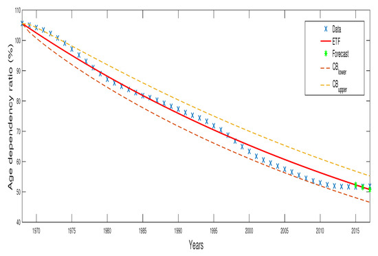  Figure 1. Observed data, estimated trend function (ETF) and the forecasted values.
  

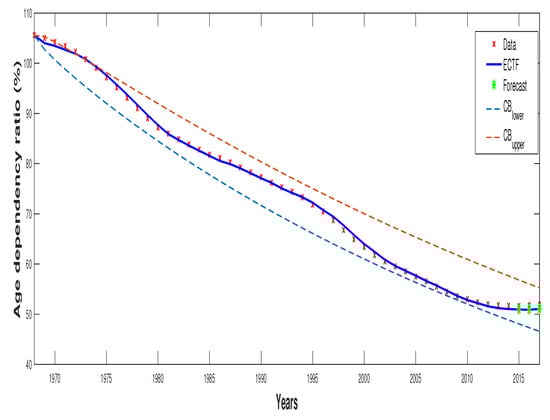  Figure 2. Observed data, estimated conditional trend function (ECTF) and the forecasted values.

5.2. Goodness of Fit

The following scale-dependent quantities are based on the absolute error or squared errors and measures based on percentage errors:

• Mean Absolute Error (MAE) = mean ($\mid e_t\mid$),
• Root Mean Square Error (RMSE) =$\sqrt{mean\left(e_t^2\right)},$
• Mean Absolute Percentage Error (MAPE) = mean ($100\ast e_t/x\left(t\right)$),

assuming $e_t=x\left(t\right)-\widehat{x}\left(t\right)$ with $\widehat{x}\left(t\right)$ is obtained by substituting the parameters in Equation (5) by their estimators.

The values obtained for the above error measures are acceptably low, especially the MAPE according to Table 3. The statistical measures obtained are illustrated in the Table 4.

Table 3. Interpretation of typical Mean Absolute Percentage Error (MAPE) values.

MAPE	Interpretation
<10	Highly accurate forecasting
20–30	Good forecasting
30–50	Reasonable forecasting
>50	Inaccurate forecasting

Table 4. Goodness of fit of the model.

MAE	RMSE	MAPE
1.6810	1.9952	2.5312%

5.3. Simulation

The sample paths were simulated by Equation (5), taking values of $\alpha$, $\beta$, ${\sigma }^2$ and $x_1$ tight to those evaluated for these parameters in the real example in the application for which this investigation was established in Section 5.1. Ten trajectories with 500 values each were generated and the following time instants considered.

Figure 3 shows the simulated trajectories of the SWDP, where the red curve represents the theoretical trend function, for the particular case of $\alpha =-0.5337,\beta =0.8457,{\sigma }^2=3.8755\times {10}^{-5}$, $h=0.096,t_1=1968,x_1=105.5770,$ which match, respectively to values near to those obtained in the study of $x\left(t\right).$

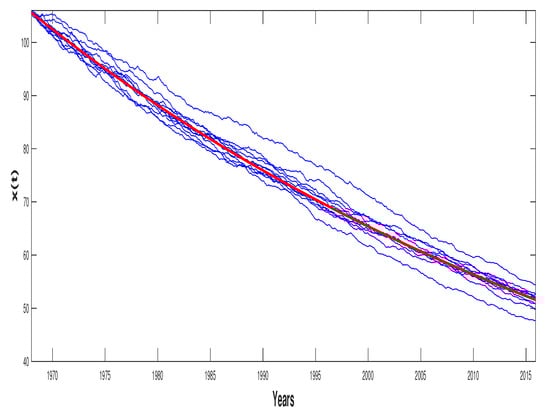
Figure 3. The Stochastic Weibull Diffusion Process (SWDP) simulated with the theoretical trend function.

6. Conclusions

The SWDP was applied to analyse the age dependency ratio in Morocco. This obtained an improved description of the time series considered (1968–2014) and improved medium-term forecasts (2015–2017). From the results obtained (see Table 2, Figure 1 and Figure 2), we deduce that when the real case considered is modelled by the SWDP model according to the estimation procedure designated in Section 3, the fit and prediction achieved, based on ETF and ECTF, present an important degree of accuracy Table 4.

From one hand, as the retirement age is stable, when the life expectancy is rising, an important part of one’s lifetime is spent in pension. On the other hand, while the birth rates is decreasing, the part of population who will afterwards represent the support to the rest of the population is going down. In view of the fact that the dependency ratio indicates how many people need to be supported relative to the number of people who are working, consequently, the increasing number of retirees and the decreasing workforce drive up the dependency ratio.

An interesting area for future research would be to examine the possibility of defining a non-homogeneous Weibull model, introducing exogenous factors into the drift, similarly to the approach adopted for other diffusions [17,18]. This would enable us to study the factors affecting the evolution of the age dependency ratio for example: fertility, immigration, mortality, health and work ability.

References

- Gutiérrez, R.; Gutiérrez-Sánchez, R.; Nafidi, A. Trend analysis and computational statistical estimation in a stochastic Rayleigh model: Simulation and application. Math. Comput. Simul. 2008, 77, 209–217. [Google Scholar] [CrossRef]
- Giovanis, A.; Skiadas, C. A stochastic logistic innovation diffusion model studying the electricity consumption in Greece and the United States. Technol. Forecast. Soc. Chang. 1999, 61, 235–246. [Google Scholar] [CrossRef]
- Gutiérrez, R.; Gutiérrez-Sánchez, R.; Nafidi, A. The Stochastic Rayleigh diffusion model: Statistical inference and computational aspects. Applications to modelling of real cases. Appl. Math. Comput. 2006, 175, 628–644. [Google Scholar] [CrossRef]
- Albano, G.; Giorno, V.; Román-Román, P.; Torres-Ruiz, F. Inferring the effect of therapy on tumors showing stochastic Gompertzian growth. J. Theor. Biol. 2011, 276, 67–77. [Google Scholar] [CrossRef] [PubMed]
- Skvortsov, A.; Ristic, B.; Kamenev, A. Predicting population extinction from early observations of the Lotka–Volterra system. Appl. Math. Comput. 2018, 320, 371–379. [Google Scholar] [CrossRef]
- Rao, B.P.; Rao, B.P. Statistical Inference for Diffusion Type Processes; Arnold: London, UK, 1999. [Google Scholar]
- Nafidi, A.; Bahij, M.; Achchab, B.; Gutiérrez-Sanchez, R. The stochastic Weibull diffusion process: Computational aspects and simulation. Appl. Math. Comput. 2019, 348, 575–587. [Google Scholar] [CrossRef]
- Kloeden, P.E.; Platen, E.; Gelbrich, M.; Romisch, W. Numerical Solution of Stochastic Differential Equations. SIAM Rev. 1995, 37, 272–274. [Google Scholar]
- Katsamaki, A.; Skiadas, C. Analytic solution and estimation of parameters on a stochastic exponential model for a technological diffusion process. Appl. Stoch. Model. Data Anal. 1995, 11, 59–75. [Google Scholar] [CrossRef]
- Zehna, P.W. Invariance of maximum likelihood estimators. Ann. Math. Stat. 1966, 37, 744. [Google Scholar] [CrossRef]
- Kirkpatrick, S.; Gelatt, C.D.; Vecchi, M.P. Optimization by Simulated Annealing. Science 1983, 220, 671–680. [Google Scholar] [CrossRef] [PubMed]
- Černỳ, V. Thermodynamical approach to the traveling salesman problem: An efficient simulation algorithm. J. Optim. Theory Appl. 1985, 45, 41–51. [Google Scholar] [CrossRef]
- Metropolis, N.; Rosenbluth, A.W.; Rosenbluth, M.N.; Teller, A.H.; Teller, E. Equation of State Calculations by Fast Computing Machines. J. Chem. Phys. 1953, 21, 1087–1092. [Google Scholar] [CrossRef]
- Duflo, M. Random Iterative Models; Springer Science & Business Media: Berlin, Germany, 2013; Volume 34. [Google Scholar]
- Boumezoued, A.; Hardy, H.L.; Karoui, N.E.; Arnold, S. Cause-of-death mortality: What can be learned from population dynamics? Insur. Math. Econ. 2018, 78, 301–315. [Google Scholar] [CrossRef]
- Boyle, P.P.; Freedman, R. Population waves and fertility fluctuations: Social security implications. Insur. Math. Econ. 1985, 4, 65–74. [Google Scholar] [CrossRef]
- Gutiérrez, R.; Gutiérrez-Sánchez, R.; Nafidi, A. Electricity consumption in Morocco: Stochastic Gompertz diffusion analysis with exogenous factors. Appl. Energy 2006, 83, 1139–1151. [Google Scholar] [CrossRef]
- Nafidi, A.; Gutiérrez, R.; Gutiérrez-Sánchez, R.; Ramos-Ábalos, E.; El Hachimi, S. Modelling and predicting electricity consumption in Spain using the stochastic Gamma diffusion process with exogenous factors. Energy 2016, 113, 309–318. [Google Scholar] [CrossRef]
© 2020 by the authors. Licensee MDPI, Basel, Switzerland. This article is an open access article distributed under the terms and conditions of the Creative Commons Attribution (CC BY) license (http://creativecommons.org/licenses/by/4.0/).