Complex Ginzburg–Landau Equation with Generalized Finite Differences

Abstract

In this paper we obtain a novel implementation for irregular clouds of nodes of the meshless method called Generalized Finite Difference Method for solving the complex Ginzburg–Landau equation. We derive the explicit formulae for the spatial derivative and an explicit scheme by splitting the equation into a system of two parabolic PDEs. We prove the conditional convergence of the numerical scheme towards the continuous solution under certain assumptions. We obtain a second order approximation as it is clear from the numerical results. Finally, we provide several examples of its application over irregular domains in order to test the accuracy of the explicit scheme, as well as comparison with other numerical methods.

1. Introduction

We address this paper to the implementation of the Generalized Finite Difference Method (GFDM) to solve the complex Ginzburg–Landau equation,

$$\left\{\begin{array}{cc}{\displaystyle \frac{\partial U}{\partial t}-(\nu +i\alpha )\Delta U+(\beta +i\mu ){\left|U\right|}^{2}U-\gamma U=0,}\hfill & \mathbf{x}\in \mathsf{\Omega },t>0,\hfill \\ U(x,y,0)=U_0(x,y),\hfill & \mathbf{x}\in \mathsf{\Omega },\hfill \\ U(x,y,t)=b(x,y,t),\hfill & \mathbf{x}\in \partial \mathsf{\Omega },t>0,\hfill \end{array}\right.$$

(1)

for some enough regular functions $U_0(x,y)$, $b(x,y,t)$ in $\mathsf{\Omega }\times [0,\infty )$, where $\mathsf{\Omega }\subset {\mathbb{R}}^2$ is a bounded domain. Here, $U(x,y,t)$ denotes a complex function, $\alpha$, $\mu$ are some real parameters and $\nu >0$, $\beta >0$. Parameter $\gamma$ is also a real number which is chosen in such a way that $U\to 0$ as $t\to \infty$, if $\gamma \le 0.$

The Equation (1) was pioneered by Ginzburg and Landau in the 1950s when the authors studied the phenomenon of phase transitions in superconductors [1]. The applications of such a theory are numerous; among others, it is a useful tool used in nonlinear dynamics, dissipative systems and some types of chemical reactions. In 1999, Wang proved the existence of at least a periodic solution to (1) in the two-dimensional setting [2].

For our numerical simulations, we use the fact that Equation (1) admits a plane-wave solution of the form

$$U(x,y,t)=\rho e^{i\left[\xi \right(x+y)-\eta t]}$$

(2)

for some real numbers $\rho$, $\xi$ and $\eta$. By a direct computation, the following system is obtained

$$\nu +\beta {\rho }^2-\gamma =0,-\eta +2\alpha {\xi }^2+\mu {\rho }^2=0,$$

(3)

whose solutions are expressed as follows

$$\xi =\pm \sqrt{{\displaystyle \frac{\gamma -\beta {\rho }^2}{2\nu }}},\eta =2\alpha {\xi }^2+\mu {\rho }^2.$$

Due to the high number of applications, several numerical studies of the Equation (1) have been carried out. For instance, finite element methods have been used since Du et al. [3], the method of Radial Basis functions was used in 2012 by Shokri and Dehghan [1] and several finite difference schemes were proposed by Wang and Dou [4]. In [5] Geiser and Nasari consider finite differences schemes and spectral methods for the spatial discretization to solve the Gross–Pitaevskii equation. Geiser in [6] presented the splitting methods that are based on iterative schemes and he applied them to the stochastic nonlinear Schrödinger equation. Geiser and Nasari in [7] use a splitting approach to solve the scale-dependent Schrödinger equations.

In [8], a finite difference scheme for the numerical solution of the Gross–Pitaevskii equation is proposed.

In this paper we propose the Generalized Finite Difference Method to solve numerically (1) and determine the behavior of the discrete solution of the numerical scheme generated by that method. This meshless method has been widely used since Lizska and Orkisz [9] and the explicit formulas of the method were derived by Benito, Gavete and Ureña [10,11,12]. The main advantage of the GFDM is the possibility of using both regular and irregular distributions (clouds) of points. The explicit formulae of the method allow us to obtain the discretization of the spatial partial derivatives. Another advantage of the method, stated in [10] is the small number of nodes at each star (8 + 1) for 2D and (26 + 1) in 3D, which results in almost empty matrices. In this way, we obtain similar computational times to the ones of classical finite difference and similar efficiency.

Thanks to its potential to solve highly nonlinear PDEs systems over irregular domains, several authors have recently used the GFDM. In [13] Wang, Gu and Liu applied the method to perform stress analysis in elastic materials in 3D and in [14,15,16] the authors have applied an explicit GFD scheme for tumor growth invasion, chemotaxis models and the Telegraph equation, respectively. We split the solution $U(x,y,t)$ into its real and imaginary parts and obtain a coupled system of two parabolic PDEs. To do so, we assume that $U(x,y,t)=F(x,y,t)+iG(x,y,t)$, for some functions $F(x,y,t),G(x,y,t)$, and, the Equation (1) becomes

$$\begin{array}{cc}\hfill & \frac{\partial F}{\partial t}=\nu \Delta F-\alpha \Delta G+\gamma F-\beta [F^2+G^2]F+\mu [F^2+G^2]G,\hfill \\ \hfill & \frac{\partial G}{\partial t}=\nu \Delta g+\alpha \Delta F+\gamma G-\beta [F^2+G^2]G-\mu [F^2+G^2]F.\hfill \end{array}$$

(4)

The conditional convergence of the explicit GFD scheme is proved.

We derive the discretization of the complex Ginzburg–Landau equation by means of the explicit formulae of the GFDM. We prove the conditional convergence of the explicit scheme by transforming the equation into a system of partial differential equations whose solutions are the real and imaginary part of the original solution. We find a condition on the time step, $\Delta t$, for the convergence of the method explicitly. In the last section of the paper we perform a comparison between our numerical results and the recent literature concerning the complex Ginzburg–Landau equation.

The paper is organized as follows: in Section 2 we present some explicit formulas using the Generalized Finite Difference method to complement the information. Then, in Section 3 we study the conditional convergence of the GFD explicit scheme, giving the explicit condition for the time step, $\Delta t$. This result is embedded in Theorem 1, which is the main result of the paper. In Section 4, extensive numerical experiments are presented to illustrate the accuracy and efficiency of the numerical algorithms developed. Finally, we present some conclusions.

2. Explicit Formulae

In order to obtain the expressions for the spatial derivatives in terms of the values of the set of nodes in the domain, let $\mathsf{\Omega }\subset {\mathbb{R}}^2$ be a domain and

$$M=\{{\mathbf{x}}_1,\dots ,{\mathbf{x}}_N\}\subset \mathsf{\Omega }$$

a discretization of $\mathsf{\Omega }$ with N points (see Figure 1). We shall denote each point of the discretization M as a node. For each one of the nodes of the domain, where the value of U is unknown, $E_s$ star is defined as a set of selected points $E_s=\{{\mathbf{x}}_0;{\mathbf{x}}_1,\dots ,{\mathbf{x}}_s\}\subset M$ with the central node ${\mathbf{x}}_0\in M$ and ${\mathbf{x}}_i(i=1,\dots ,s)\in M$ is a set of points located in the neighborhood of ${\mathbf{x}}_0$. In order to select the points, different criteria as four quadrants or distance can be used [10].

Let ${\mathbf{x}}_0=(x_0,y_0)$ be the central node of a $E_s$ star and $h_i=x_i-x_0$, $k_i=y_i-y_0$, where $(x_i,y_i)$ are the coordinates of the ith node of $E_s.$ Let us put $U_0=U\left({\mathbf{x}}_0\right)$ and $U_i=U\left({\mathbf{x}}_i\right),$ then by the Taylor series expansion for the spatial variables, we have

$$U_i=U_0+h_i{\displaystyle \frac{\partial U_0}{\partial x}}+k_i{\displaystyle \frac{\partial U_0}{\partial y}}+{\displaystyle \frac{1}{2}}\left(h_i^2{\displaystyle \frac{{\partial }^2{U}_0}{\partial x^2}}+k_i^2{\displaystyle \frac{{\partial }^2{U}_0}{\partial y^2}}+2h_i{k}_i{\displaystyle \frac{{\partial }^2{U}_0}{\partial x\partial y}}\right)+\dots$$

(5)

for $i=1,\dots ,s$. Let us call

$${{\mathbf{c}}_i}^T=\{h_i,k_i,\frac{h_i^2}{2},\frac{k_i^2}{2},h_i{k}_i\},$$

$${\mathit{D}}_{\mathbf{5}}^T=\{\frac{\partial u_0}{\partial x},\frac{\partial u_0}{\partial y},\frac{{\partial }^2{u}_0}{\partial x^2},\frac{{\partial }^2{u}_0}{\partial y^2},\frac{{\partial }^2{u}_0}{\partial x\partial y}\},$$

where we use the notation $\frac{{\partial }^j{u}_0}{\partial x^j}$ for the approximated value of the j-order spatial derivative of $U\left(\mathbf{x}\right)$ evaluated at ${\mathbf{x}}_0$. If in (5) we do not consider the higher than second order terms, we can obtain a second order approximation of $U_i$, which we shall denote by $u_i$. Then, we define the following:

$$\begin{array}{cc}{\displaystyle B\left(u\right)=\sum _{i=1}^s}& \left[(u_0-u_i)+h_i\frac{\partial u_0}{\partial x}+k_i\frac{\partial u_0}{\partial y}\right.+\hfill \\ & {\left.+\frac{1}{2}(h_i^2\frac{{\partial }^2{u}_0}{\partial x^2}+k_i^2\frac{{\partial }^2{u}_0}{\partial y^2}+2h_i{k}_i\frac{{\partial }^2{u}_0}{\partial x\partial y})\right]}^2{w}_i^2,\hfill \end{array}$$

(6)

where $w_i=w(h_i,k_i)$ are positive symmetrical weighting functions which decrease in magnitude as the distance to the center increases, as defined in Lankaster and Salkauskas [17]. Some weighting functions as potentials or exponential can be used (see [18] for more details). We can minimize the norm given by (6) with respect to the partial derivatives by considering the following linear system

$$\mathit{A}(h_i,k_i,w_i){\mathit{D}}_{\mathbf{5}}=\mathit{b}(h_i,k_i,w_i,u_0,u_i),$$

where

$$\mathit{A}=\left(\begin{array}{cccc}{h}_1& h_2& \cdots & h_s\\ k_1& k_2& \cdots & k_s\\ ⋮& ⋮& ⋮& ⋮\\ h_1{k}_1& h_2{k}_2& \cdots & h_s{k}_s\end{array}\right)\left(\begin{array}{cccc}{\omega }_1^2& & & \\ & {\omega }_2^2& & \\ & & \cdots & \\ & & & {\omega }_s^2\end{array}\right)\left(\begin{array}{cccc}{h}_1& k_1& \cdots & h_1{k}_1\\ h_2& k_2& \cdots & h_2{k}_2\\ ⋮& ⋮& ⋮& ⋮\\ h_s& k_s& \cdots & h_s{k}_s\end{array}\right),$$

and

$$\begin{array}{cc}{\mathit{b}}^T=\hfill & {\displaystyle \left(\sum _{i=1}^s(-u_0+u_i)h_i{w}_i^2,\sum _{i=1}^s(-u_0+u_i)k_i{w}_i^2,\sum _{i=1}^s(-u_0+u_i)\frac{h_i^2{w}_i^2}{2},\right.}\hfill \\ \hfill & {\displaystyle \left.\sum _{i=1}^s(-u_0+u_i)\frac{k_i^2{w}_i^2}{2},\sum _{i=1}^s(-u_0+u_i)h_i{k}_i{w}_i^2\right).}\hfill \end{array}$$

It is well known that $\mathit{A}$ is a positive definite matrix and the approximation is of second order $\mathsf{\Theta }(h_i^2,k_i^2)$ (see [18,19]).

If we define

$${\mathit{A}}^{-1}=\mathit{Q}{\mathit{Q}}^T,$$

we have

$${\mathit{D}}_{\mathbf{5}}=\mathit{Q}{\mathit{Q}}^T\mathit{b}.$$

(7)

Thus, Equation (7) can be rewritten as

$${\displaystyle {\mathit{D}}_{\mathbf{5}}=-u_0\mathit{Q}{\mathit{Q}}^T\sum _{i=1}^s{w}_i^2{\mathit{c}}_{\mathit{i}}+\mathit{Q}{\mathit{Q}}^T\sum _{i=1}^s{u}_i{w}_i^2{\mathit{c}}_{\mathit{i}},}$$

or

$$\mathit{D}=\mathit{Q}{\mathit{Q}}^T\mathit{W}(\mathit{u}-u_0\mathbf{1})$$

where

$$\mathit{W}=\left(\begin{array}{cccc}{h}_1{w}_1^2& h_2{w}_2^2& \cdots & h_s{w}_s^2\\ k_1{w}_1^2& k_2{w}_2^2& \cdots & k_s{w}_s^2\\ \frac{h_1^2}{2}{w}_1^2& \frac{h_2^2}{2}{w}_2^2& ⋮& \frac{h_s^2}{2}{w}_s^2\\ \frac{k_1^2}{2}{w}_1^2& \frac{k_2^2}{2}{w}_2^2& ⋮& \frac{k_s^2}{2}{w}_s^2\\ h_1{k}_1{w}_1^2& h_2{k}_2{w}_s^2& \cdots & h_s{k}_s{w}_s^2\end{array}\right)$$

and

$$\mathbf{1}=\left\{1,1,\cdots ,1\right\};\mathit{u}={\left\{u_1,u_2,\cdots ,u_s\right\}}^T.$$

Thus, the spatial derivatives using GFD, as in [20], are denoted by

$$\left\{\begin{array}{c}{\displaystyle {\displaystyle \frac{{\partial }^{2}u({\mathbf{x}}_0,n▵t)}{\partial x^2}}=-m_{03}{u}_0+\sum _{i=1}^s{m}_{i3}{u}_i+\mathsf{\Theta }(h_i^2,k_i^2),\mathrm{with}{m}_{03}=\sum _{i=1}^s{m}_{i3},}\hfill \\ {\displaystyle {\displaystyle \frac{{\partial }^{2}u({\mathbf{x}}_0,n▵t)}{\partial y^2}}=-m_{04}{u}_0+\sum _{i=1}^s{m}_{i4}{u}_i+\mathsf{\Theta }(h_i^2,k_i^2),\mathrm{with}{m}_{04}=\sum _{i=1}^s{m}_{i4}.}\hfill \end{array}\right.$$

(8)

We can rewrite (8) in the equivalent vectorial form,

$${\mathit{D}}_{\mathbf{5}}u({\mathbf{x}}_0,n\Delta t)=-{\mathit{m}}_{\mathbf{0}}{u}_0+\sum _{i=1}^s{\mathit{m}}_{\mathit{i}}{u}_i+\mathsf{\Theta }(h_i^2,k_i^2),$$

where ${\mathit{m}}_{\mathbf{0}}$ and ${\mathit{m}}_{\mathit{i}}$ stand for

$$\begin{array}{c}\hfill {\mathit{m}}_{\mathbf{0}}={\{m_{01},m_{02},m_{03},m_{04},m_{05}\}}^T,\\ \hfill {\mathit{m}}_{\mathit{i}}={\{m_{i1},m_{i2},m_{i3},m_{i4},m_{i5}\}}^T,\\ \hfill m_{00}=m_{03}+m_{04};m_{i0}=m_{i3}+m_{i4},\end{array}$$

are fulfilling

$${\mathit{m}}_{\mathbf{0}}=\sum _{i=1}^s{\mathit{m}}_{\mathit{i}}.$$

3. GFDM Schemes

The discretization of Equation (1) can be expressed as

$$\begin{array}{cc}\hfill \frac{u_0^{n+1}-u_0^n}{\Delta t}=& \nu \left(-m_{00}{u}_0^n+\sum _{i=1}^s{m}_{0i}{u}_i^n\right)+\gamma u_0^n-\beta {\left|u_0^n\right|}^2{u}_0^n\hfill \\ & +i\left[-\alpha \left(-m_{00}{u}_0^n+\sum _{i=1}^s{m}_{0i}{u}_i^n\right)-\mu {\left|u_0^n\right|}^2{u}_0^n\right]+\mathsf{\Theta }(\Delta t,h_i^2,k_i^2).\hfill \end{array}$$

(9)

We transcribe (9) by means of the real and imaginary parts of the discrete solution, i.e., $u^n=f^n+i{g}^n$,

$$\begin{array}{cc}\hfill \frac{(f_0^{n+1}+i{g}_0^{n+1})-(f_0^n+i{g}_0^n)}{\Delta t}=& \nu \left(-m_{00}(f_0^n+i{g}_0^n)+\sum _{i=1}^s{m}_{0i}(f_i^n+i{g}_i^n)\right)+\gamma (f_0^n+i{g}_0^n)\hfill \\ & -\beta |(f_0^n+i{g}_0^n){|}^2(f_0^n+i{g}_0^n)\hfill \\ & +i[-\alpha \left(-m_{00}(f_0^n+i{g}_0^n)+\sum _{i=1}^s{m}_{0i}(f_i^n+i{g}_i^n)\right)\hfill \\ & -\mu |(f_0^n+i{g}_0^n){|}^2(f_0^n+i{g}_0^n)]+\mathsf{\Theta }(\Delta t,h_i^2,k_i^2)\hfill \end{array}$$

(10)

and we break the equation into two parts by taking the following system

$$\begin{array}{cc}\hfill \frac{f_0^{n+1}-f_0^n}{\Delta t}=& -\nu m_{00}{f}_0^n+\nu \sum _{i=1}^s{m}_{0i}{f}_i^n+\gamma f_0^n-\beta [{\left(f_0^n\right)}^2+{\left(g_0^n\right)}^2]f_0^n\hfill \\ \hfill & +\alpha m_{00}{g}_0^n-\alpha \sum _{i=1}^s{m}_{0i}{g}_i^n+\mu [{\left(f_0^n\right)}^2+{\left(g_0^n\right)}^2]g_0^n+\mathsf{\Theta }(\Delta t,h_i^2,k_i^2).\hfill \end{array}$$

(11)

$$\begin{array}{cc}\hfill \frac{g_0^{n+1}-g_0^n}{\Delta t}=& -\nu m_{00}{g}_0^n+\nu \sum _{i=1}^s{m}_{0i}{g}_i^n+\gamma g_0^n-\beta [{\left(f_0^n\right)}^2+{\left(g_0^n\right)}^2]g_0^n\hfill \\ \hfill & -\alpha m_{00}{f}_0^n+\alpha \sum _{i=1}^s{m}_{0i}{f}_i^n-\mu [{\left(f_0^n\right)}^2+{\left(g_0^n\right)}^2]f_0^n+\mathsf{\Theta }(\Delta t,h_i^2,k_i^2),\hfill \end{array}$$

(12)

For the purpose of proving the main result of the paper concerning the conditional convergence of the GFD scheme to solve system (1), we need the following basic results from Isaacson and Keller [21] [Section 1.1, Theorem 4 and the following Corollary].

Lemma 1.

Let $N\in {\mathfrak{M}}_{n\times n}\left(\mathbb{R}\right)$. If there exists some matrix norm such that $\parallel N\parallel <1,$ then

$$\underset{k\to \infty }{lim}{N}^k=\mathbf{0}.$$

Lemma 2.

Assume $N\in {\mathfrak{M}}_{n\times n}\left(\mathbb{R}\right)$, then the following statements are equivalent

i. 

${\displaystyle \underset{k\to \infty }{lim}{N}^k=\mathbf{0},}$

ii. 

$\rho \left(N\right)<1$,

where $\rho (·)$ stands for the spectral radius.

Theorem 1.

Let $U=F+iG$ be the solution of (1). Assume that $F,G\in C^4\left(\overline{\mathsf{\Omega }}\right)$, and α, β, γ, μ, ν are real constants. Under the following condition

$$\Delta t\le 2min\left\{{\displaystyle {\displaystyle \frac{1}{{\displaystyle m_{00}+\left|A\right|+\left|B\right|+(\nu +\alpha )\sum _{i=1}^s\left|m_{0i}\right|}}},{\displaystyle \frac{1}{{\displaystyle m_{00}+\left|C\right|+\left|D\right|+(\nu +\alpha )\sum _{i=1}^s\left|m_{0i}\right|}}}}\right\},$$

(13)

the explicit scheme given by (11) and (12) is conditionally convergent, where

$$A:={\nu }^{-1}\left[-\gamma +\beta [{\left(f_0^n\right)}^2+f_0^n{F}_0^n+{\left(F_0^n\right)}^2]+\beta {\left(g_0^n\right)}^2+\mu G_0^n(f_0^n+F_0^n)]\right],$$

$$B:=\left[\alpha m_{00}-\beta F_0^n(g_0^n+G_0^n)+\mu {\left(f_0^n\right)}^2+\mu [{\left(g_0^n\right)}^2+g_0^n{G}_0^n+{\left(G_0^n\right)}^2]\right],$$

$$C:={\nu }^{-1}\left[-\gamma +\beta [{\left(g_0^n\right)}^2+g_0^n{G}_0^n+{\left(F_0^n\right)}^2]+\beta {\left(f_0^n\right)}^2\mu F_0^n(g_0^n+G_0^n)]\right],$$

$$D:=\left[-\alpha m_{00}-\beta G_0^n(f_0^n+F_0^n)-\mu {\left(g_0^n\right)}^2-\mu [{\left(f_0^n\right)}^2+f_0^n{F}_0^n+{\left(F_0^n\right)}^2]\right].$$

Proof. 

To check the conditional convergence of the explicit scheme given by (11) and (12), we take the difference between such expressions, that is, for the discrete solution we use the notation $f_i^n$ and for the exact solution, $F_i^n$. We call, ${\tilde{f}}_i^n=f_i^n-F_i^n,$${\tilde{g}}_i^n=g_i^n-G_i^n$. For the real part, we have

$$\begin{array}{cc}\hfill \frac{{\tilde{f}}_0^{n+1}-{\tilde{f}}_0^n}{\Delta t}=& {\tilde{f}}_0^n(-\nu m_{00}+\gamma )+\nu \sum _{i=1}^s{m}_{0i}{\tilde{f}}_i^n+\alpha m_{00}{\tilde{g}}_0^n-\alpha \sum _{i=1}^s{m}_{0i}{\tilde{g}}_i^n\hfill \\ \hfill & +(-\beta f_0^n+\mu g_0^n)[{\left(f_0^n\right)}^2+{\left(g_0^n\right)}^2]-(-\beta F_0^n+\mu G_0^n)[{\left(F_0^n\right)}^2+{\left(G_0^n\right)}^2].\hfill \end{array}$$

(14)

For the last term of (14) we have

$$-\beta {\left(f_0^n\right)}^3+\beta {\left(F_0^n\right)}^3=-\beta {\tilde{f}}_0^n[{\left(f_0^n\right)}^2+f_0^n{F}_0^n+{\left(F_0^n\right)}^2]$$

(15)

and

$$-\beta f_0^n{\left(g_0^n\right)}^2+\beta F_0^n{\left(G_0^n\right)}^2\pm \beta F_0^n{\left(g_0^n\right)}^2=-\beta {\tilde{f}}_0^n{\left(g_0^n\right)}^2-\beta F_0^n(g_0^n+G_0^n){\tilde{g}}_0^n.$$

(16)

In the same way, we obtain

$$\mu g_0^n{\left(f_0^n\right)}^2-\mu G_0^n{\left(F_0^n\right)}^2=\mu {\tilde{g}}_0^n{\left(f_0^n\right)}^2+\mu G_0^n(f_0^n+F_0^n){\tilde{f}}_0^n.$$

(17)

Finally, we get

$$\mu {\left(g_0^n\right)}^3-\mu {\left(G_0^n\right)}^3=\mu \widetilde{g_0^n}[{\left(g_0^n\right)}^2+g_0^n{G}_0^n+{\left(G_0^n\right)}^2].$$

(18)

Using (15)–(18) in (14), we arrive to

$$\begin{array}{cc}\hfill \frac{{\tilde{f}}_0^{n+1}-{\tilde{f}}_0^n}{\Delta t}& ={\tilde{f}}_0^n\left[-\nu m_{00}+\gamma -\beta [{\left(f_0^n\right)}^2+f_0^n{F}_0^n+{\left(F_0^n\right)}^2]-\beta {\left(g_0^n\right)}^2+\mu G_0^n(f_0^n+F_0^n)]\right]\hfill \\ & +{\tilde{g}}_0^n\left[\alpha m_{00}-\beta F_0^n(g_0^n+G_0^n)+\mu {\left(f_0^n\right)}^2+\mu [{\left(g_0^n\right)}^2+g_0^n{G}_0^n+{\left(G_0^n\right)}^2]\right]\hfill \\ \hfill & +\nu \sum _{i=1}^s{m}_{0i}{\tilde{f}}_i^n-\alpha \sum _{i=1}^s{m}_{0i}{\tilde{g}}_i^n.\hfill \end{array}$$

(19)

Hence, it yields

$${\tilde{f}}^{n+1}={\tilde{f}}_0^n-\nu \Delta t(m_{00}+A){\tilde{f}}_0^n+\Delta t\nu \sum _{i=1}^s{m}_{0i}{\tilde{f}}_i^n+\Delta t{\tilde{g}}_0^{n}B-\Delta t\alpha \sum _{i=1}^s{m}_{0i}{\tilde{g}}_i^n,$$

(20)

for some A and B known clearly given in (19) after rearranging. Now, by calling ${\displaystyle {\tilde{f}}^n=\underset{i\in \{0,...,s\}}{max}\left\{\right|{\tilde{f}}_i^n\left|\right\}}$ and ${\displaystyle {\tilde{g}}^n=\underset{i\in \{0,...,s\}}{max}\left\{\right|{\tilde{g}}_i^n\left|\right\}}$, we obtain the inequality

$${\tilde{f}}^{n+1}\le {\tilde{f}}^n\left(|1-\Delta t(m_{00}+A)|+\Delta t\nu \sum _{i=1}^s\left|m_{0i}\right|\right)+{\tilde{g}}^n\left(\Delta t\left|B\right|+\Delta t\alpha \sum _{i=1}^s\left|m_{0i}\right|\right).$$

(21)

Through similar arguments, for the second equation of (12), one gets

$${\tilde{g}}^{n+1}\le {\tilde{g}}^n\left(|1-\Delta t(m_{00}+C)|+\Delta t\nu \sum _{i=1}^s\left|m_{0i}\right|\right)+{\tilde{f}}^n\left(\Delta t\left|D\right|+\Delta t\alpha \sum _{i=1}^s\left|m_{0i}\right|\right).$$

(22)

The Equations (21) and (22) can be rearranged in matrix form as

$$\left(\begin{array}{c}{\tilde{f}}^{n+1}\\ {\tilde{g}}^{n+1}\end{array}\right)\le M\left(\begin{array}{c}{\tilde{f}}^n\\ {\tilde{g}}^n\end{array}\right),$$

(23)

where matrix M is given by

$$M=\left(\begin{array}{cc}{\displaystyle |1-\Delta t(m_{00}+A)|+\Delta t\nu \sum _{i=1}^s\left|m_{0i}\right|}& {\displaystyle \Delta t\left|B\right|+\Delta t\alpha \sum _{i=1}^s\left|m_{0i}\right|}\\ {\displaystyle \Delta t\left|D\right|+\Delta t\alpha \sum _{i=1}^s\left|m_{0i}\right|}& {\displaystyle |1-\Delta t(m_{00}+C)|+\Delta t\nu \sum _{i=1}^s\left|m_{0i}\right|}\end{array}\right).$$

(24)

Now consider the ${\parallel ·\parallel }_1$ matrix norm defined as the maximum sum per row and note that if ${\parallel M\parallel }_1$ corresponds to the first row

$$|1-\Delta t(m_{00}+A)|+\Delta t\nu \sum _{i=1}^s|m_{0i}|+\Delta t|B|+\Delta t\alpha \sum _{i=1}^s\left|m_{0i}\right|<1$$

(25)

is equivalent to

$$|1-\Delta t{m}_{00}|<1-\Delta t\left[\left|A\right|+(\nu +\alpha )\sum _{i=1}^s|m_{0i}|+|B|\right]$$

(26)

and the last inequality holds since by assumption

$$\Delta t<{\displaystyle \frac{2}{{\displaystyle m_{00}+\left|A\right|+\left|B\right|+(\nu +\alpha )\sum _{i=1}^s\left|m_{0i}\right|}}}.$$

(27)

If ${\parallel M\parallel }_1$ corresponds to the second row, the condition in this case is

$$\Delta t<{\displaystyle \frac{2}{{\displaystyle m_{00}+\left|C\right|+\left|D\right|+(\nu +\alpha )\sum _{i=1}^s\left|m_{0i}\right|}}}.$$

(28)

Now, both are holding by assumption (13). Finally, applying the Lemmas 1 and 2 the proof of the conditional convergence is hereby completed. □

4. Numerical Results

In this section we present the numerical results obtained by solving the system (1), using the three irregular clouds of points shown in Figure 1 over the domain $\mathsf{\Omega }\subset [0,1]\times [0,1]$. Note the boundary of the domain $\mathsf{\Omega }$ is irregular and the distribution of the nodes is also irregular. With election of the domain and the clouds of nodes we make clear the potential of the method stated in the introduction. We present a comparison between the results obtained by using the GFDM in this paper and the ones obtained in [1,22]. The first cloud, with 55 nodes, is obtained by distributing the points randomly and deleting the ones which are sufficiently near. We generate the second cloud, with 197 nodes, by inserting points at the midpoints of the existing nodes. In the same way we obtain the third cloud of 743 points. We use a scheme of eight nodes, chosen by the criterion of distance together with the weight function $w={\displaystyle \frac{1}{dis{t}^4}}$. For all the numerical examples we put $\Delta t=0.001.$

For the following examples we choose as parameters of the equation $\nu =1$, $\alpha =0.2$, $\beta =1$, $\mu =2$ and $\gamma =1+\frac{2{\pi }^2}{9}$. As stated in the introduction, Equation (1) admits a solution of the form

$$U(x,y,t)=e^{i[\frac{\pi }{3}(x+y)-2(1+\frac{2{\pi }^2}{9})t]}$$

(29)

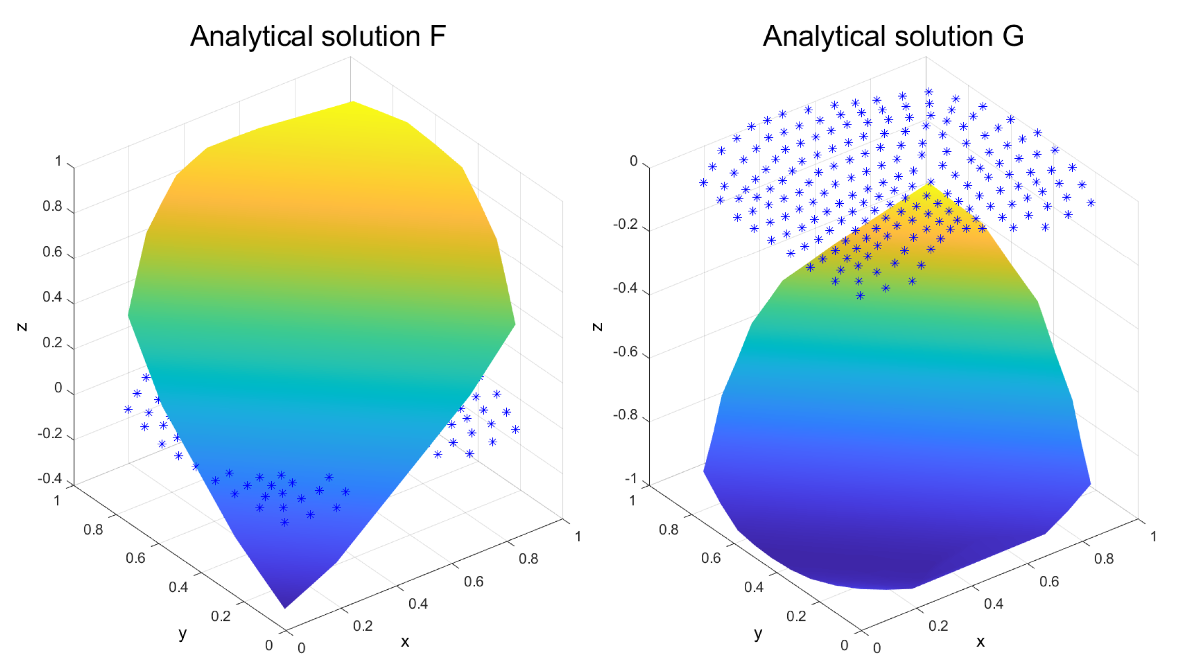
where we put $\rho =1$, $\xi =\frac{\pi }{3}$ and $\eta =2(1+\frac{2{\pi }^2}{9})$, clearly verifying condition (3). A plot of the solution is given in Figure 2 (where both real and imaginary parts can be found). As initial data we use, evidently,

$$U_0(x,y)=e^{i\frac{\pi }{3}(x+y)}.$$

For all the following figures, we plot the numerical solutions at $t=2$ s.

4.1. Example 1

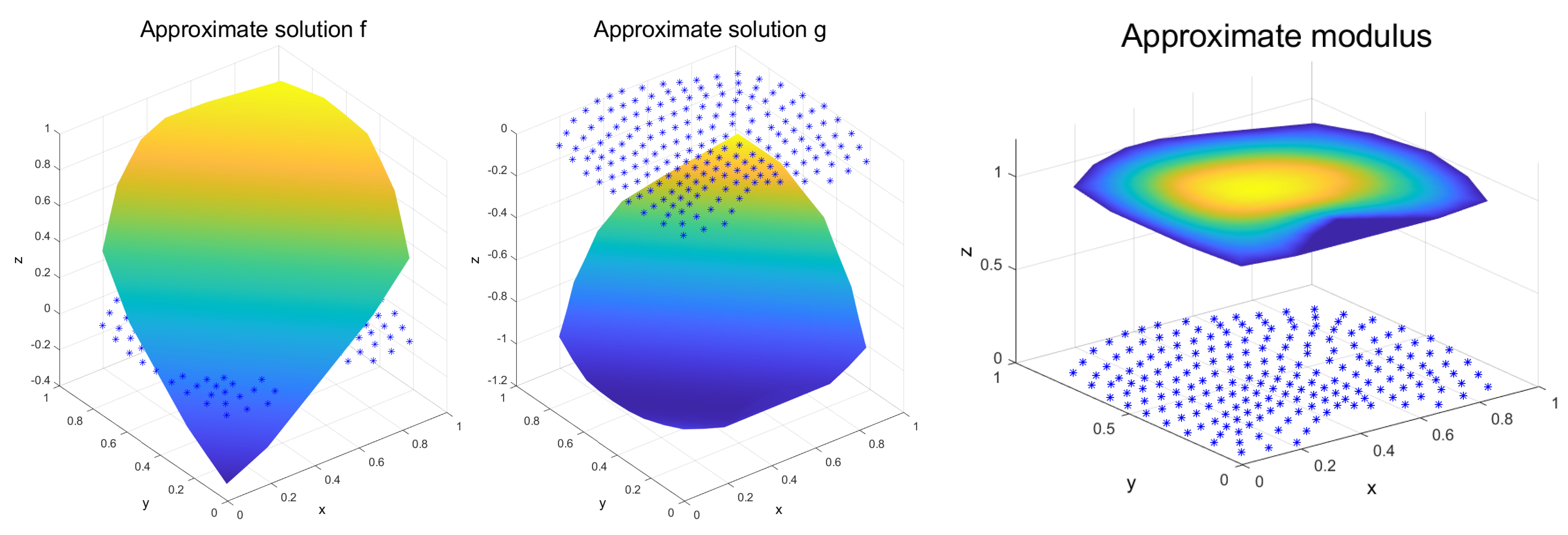
We use the first cloud of points in Figure 1 (55 nodes), and outline in Figure 3 the approximate real and imaginary parts (f and g, respectively), as well as the modulus of the solutions. The norms $l^2$ and $l^{\infty }$ of the discrete real and imaginary parts at different times are displayed in

Table 1. $l^2$ and $l^{\infty }$ norms of the errors of the real parts, respectively.

t (s)	0.25	0.5	2
cloud 1 (55 nodes)	$4.5857\times {10}^{-4}$	$1.9445\times {10}^{-4}$	$1.3043\times {10}^{-4}$
cloud 2 (197 nodes)	$1.2661\times {10}^{-4}$	$5.429\times {10}^{-5}$	$3.438\times {10}^{-5}$
cloud 3 (743 nodes)	$3.356\times {10}^{-5}$	$1.434\times {10}^{-5}$	$8.910\times {10}^{-6}$
t (s)	0.25	0.5	2
cloud 1 (55 nodes)	$5.7601\times {10}^{-4}$	$4.0733\times {10}^{-4}$	$2.0545\times {10}^{-4}$
cloud 2 (197 nodes)	$1.6104\times {10}^{-4}$	$1.1307\times {10}^{-4}$	$5.735\times {10}^{-5}$
cloud 3 (743 nodes)	$4.237\times {10}^{-5}$	$3.010\times {10}^{-5}$	$1.521\times {10}^{-5}$

and

Table 2. $l^2$ and $l^{\infty }$ norms of the errors of the imaginary parts, respectively.

t (s)	0.25	0.5	2
cloud 1 (55 nodes)	$2.0933\times {10}^{-4}$	$1.4701\times {10}^{-4}$	$8.135\times {10}^{-5}$
cloud 2 (197 nodes)	$5.844\times {10}^{-5}$	$4.105\times {10}^{-5}$	$2.271\times {10}^{-5}$
cloud 3 (743 nodes)	$1.549\times {10}^{-5}$	$1.090\times {10}^{-5}$	$6.02\times {10}^{-6}$
t (s)	0.25	0.5	2
cloud 1 (55 nodes)	$4.7223\times {10}^{-4}$	$1.5984\times {10}^{-4}$	$9.024\times {10}^{-5}$
cloud 2 (197 nodes)	$1.3201\times {10}^{-4}$	$4.486\times {10}^{-5}$	$2.521\times {10}^{-5}$
cloud 3 (743 nodes)	$3.495\times {10}^{-5}$	$1.198\times {10}^{-5}$	$6.70\times {10}^{-6}$

, respectively. We emphasize that the results obtained confirm numerically, under the hypothesis of Theorem 1, the convergence of the solution of the numerical scheme.

4.2. Example 2

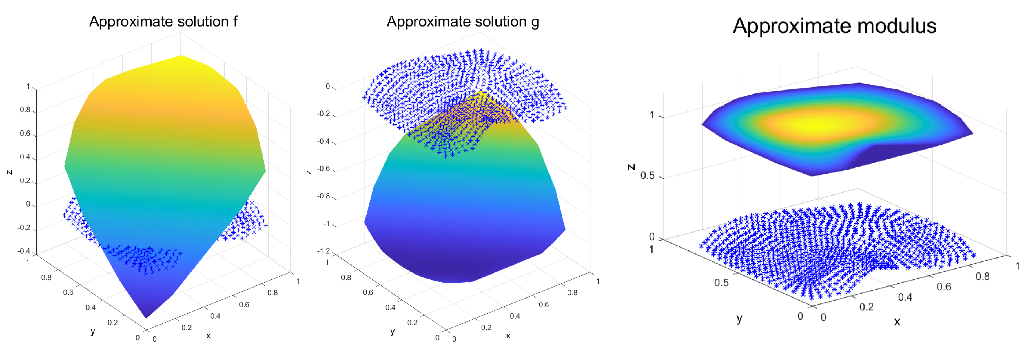
Similarly to Example 1, for the second cloud of points of Figure 1 (197 nodes) we illustrate in Table 1 and Table 2 the error in the real and imaginary parts (f and g, respectively) using the $l^2$ and $l^{\infty }$ norms. Moreover, Figure 4 represents the approximate real and imaginary parts, together with the modulus of the discrete solution.

4.3. Example 3

We use the third cloud of points of Figure 1 (743 nodes), and display in Figure 5 the approximate real, imaginary parts (f and g, respectively) and the modulus of the solutions. The $l^2$ and $l^{\infty }$ norms of the real part at different times are tabulated in Table 1 and Table 2, as well as the imaginary parts.

Remark 1.

The previous results are in the range of the recent literature concerning the application of computational methods for solving the complex Ginzburg–Landau equation. For instance, in [1], the authors used the Radial Basis Functions method, for $t=2$ s, and the errors are in accordance with our numerical examples. In addition, in [22], the authors use several compact finite difference schemes and their results are similar to ours, as it is clear from

Table 3. $l^2$ and $l^{\infty }$ norms of the errors of the papers [1,22].

t (s)	Results in [1]	Results in [22]
$l^2$	$2.39\times {10}^{-1}$	$8.76\times {10}^{-5}$
$l^{\infty }$	$1.63\times {10}^{-4}$	$2.09\times {10}^{-5}$

.

The following tables (

Table 4. Convergence order computed in $l^2$ and $l^{\infty }$ norms for the real parts, respectively.

t (s)	0.25	0.5	2
${\displaystyle \frac{{\mathrm{error}}_1}{{\mathrm{error}}_2}}$	3.6219	3.5817	3.7938
${\displaystyle \frac{{\mathrm{error}}_2}{{\mathrm{error}}_3}}$	3.7726	3.7859	3.8585
t (s)	0.25	0.5	2
${\displaystyle \frac{{\mathrm{error}}_1}{{\mathrm{error}}_2}}$	3.5768	3.6024	3.5824
${\displaystyle \frac{{\mathrm{error}}_2}{{\mathrm{error}}_3}}$	3.8008	3.7565	3.7705

and

Table 5. Convergence order computed in $l^2$ and $l^{\infty }$ norms for the imaginary parts, respectively.

t (s)	0.25	0.5	2
${\displaystyle \frac{{\mathrm{error}}_1}{{\mathrm{error}}_2}}$	3.5819	3.5812	3.5821
${\displaystyle \frac{{\mathrm{error}}_2}{{\mathrm{error}}_3}}$	3.7727	3.7661	3.7724
t (s)	0.25	0.5	2
${\displaystyle \frac{{\mathrm{error}}_1}{{\mathrm{error}}_2}}$	3.5772	3.5631	3.5795
${\displaystyle \frac{{\mathrm{error}}_2}{{\mathrm{error}}_3}}$	3.7771	3.7446	3.7627

) collect the numerical convergence order for the three previous clouds and times 0.25, 0.5 and 2 s, computed as $\frac{{\mathrm{error}}_{i-1}}{{\mathrm{error}}_i}$.

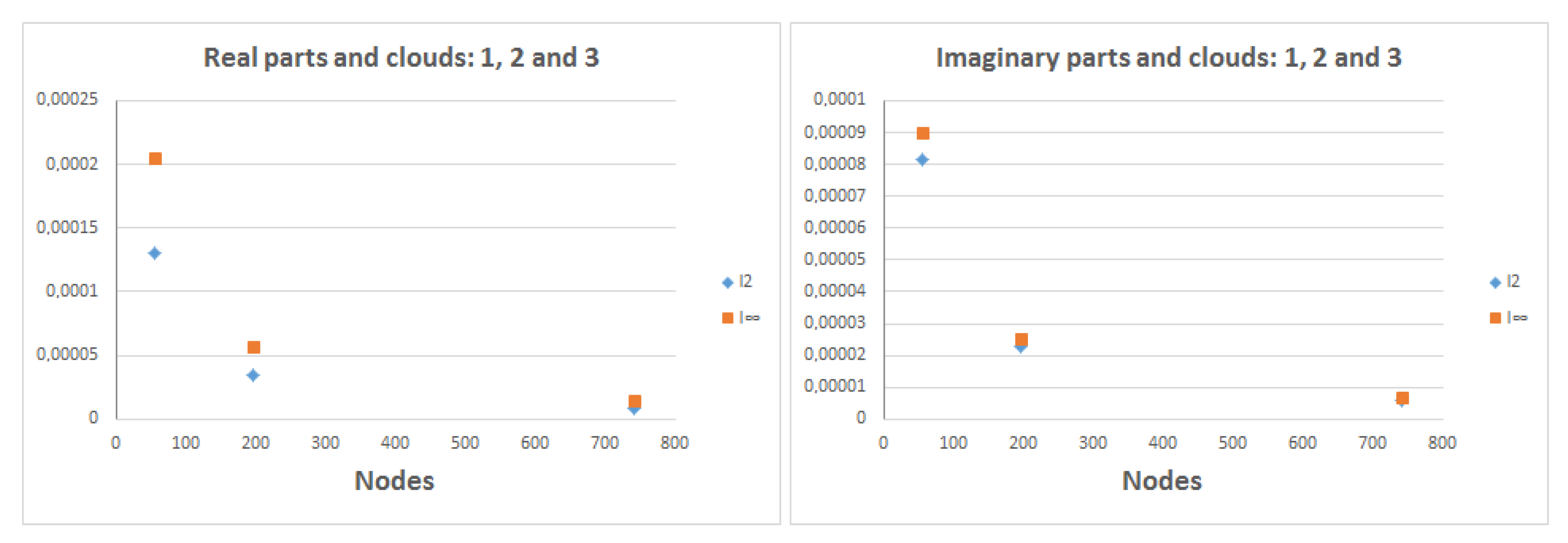
Taking into account the cloud generation (introducing new nodes in the midpoint of some previous points), we can observe that the error decreases four times, approximately. That is to say, the convergence is quadratic. It is also worth noting that we obtain similar values in the two defined norms.

Figure 6 outlines the variation of the error of the real and imaginary discrete solution vs. the number of nodes of the three clouds for $t=2$ s. It can be checked that the convergence is quadratic. In Figure 7 we show both error norms against time. We observe that the values of these norms decrease as the time increases. Note that we compute the solution at small times, which can explain the behavior of the error.

Remark 2.

The previous results are in the range of the recent literature concerning the application of computational methods for solving the complex Ginzburg–Landau equation. For instance, in [1], the authors used the Radial Basis Functions method, for $t=2$ s, and the errors are in accordance with our numerical examples.

5. Conclusions

We have applied the explicit formulas of the Generalized Finite Difference Method to solve the complex Ginzburg–Landau equation. We have transformed (1) it into a system of coupled parabolic PDEs and derived the explicit scheme using the GFDM. In Theorem 1, we have obtained under which conditions for the time step, $\Delta t$, the numerical solution converges to the continuous one.

Several examples on rather irregular domains are given to illustrate the main outcome of the work. These examples are used to verify the method by comparing the discrete solution with the one given by (2). As it is clear from the error obtained, this meshless method can be used to numerically solve the complex Ginzburg–Landau equation with great precision and efficiency over domains of complicated geometry and irregular node distribution.

References

1. Shokri, A.; Dehghan, M. A Meshless Method Using Radial Basis Functions for the Numerical Solution of Two-Dimensional Complex Ginzburg-Landau Equation. CMES Comput. Model. Eng. Sci. 2012, 84, 333–358. [Google Scholar]
2. Wang, B. Existence of Time Periodic Solutions for the Ginzburg-Landau Equations of Superconductivity. J. Math. Anal. Appl. 1999, 232, 394–412. [Google Scholar] [CrossRef] [Green Version]
3. Du, Q.; Gunburger, M.D.; Peterson, J.S. Modeling and Analysis of a Periodic Ginzburg–Landau Model for Type-II Superconductors. SIAM J. Appl. Math. 1992, 53, 689–717. [Google Scholar] [CrossRef]
4. Wang, T.; Guo, B. Analysis of some finite difference schemes for two?dimensional Ginzburg-Landau equation. Numer. Methods Partial Differ. Equ. 2011, 25, 1340–1363. [Google Scholar] [CrossRef]
5. Geiser, J.; Nasari, A. Comparison of Splitting Methods for Deterministic/Stochastic Gross-Pitaevskii Equation. Math. Comput. Appl. 2019, 24, 76. [Google Scholar] [CrossRef] [Green Version]
6. Geiser, J. Iterative Splitting Method as Almost Asymptotic Symplectic Integrator for Stochastic Nonlinear Schrödinger Equation. AIP Conf. Proc. 2017, 1863, 560005. [Google Scholar] [CrossRef]
7. Geiser, J.; Nasari, A. Simulation of multiscale Schrödinger equation with extrapolated splitting approaches. AIP Conf. Proc. 2019, 2116, 450006. [Google Scholar] [CrossRef]
8. Trofimov, V.A.; Peskov, N.V. Comparison of finite difference schemes for the Gross-Pitaevskii equation. Math. Model. Anal. 2009, 14, 109–126. [Google Scholar] [CrossRef]
9. Liszka, T.; Orkisz, J. The finite difference method at arbitrary irregular grids and its application in applied mechanics. Comput. Struct. 1980, 11, 83–95. [Google Scholar] [CrossRef]
10. Benito, J.J.; Ureña, F.; Gavete, L. Influence of several factors in the generalized finite difference method. Appl. Math. Model. 2001, 25, 1039–1053. [Google Scholar] [CrossRef]
11. Gavete, L.; Benito, J.J.; Ureña, F. Generalized finite differences for solving 3D elliptic and parabolic equations. Appl. Math. Model. 2016, 40, 955–965. [Google Scholar] [CrossRef]
12. Ureña, F.; Benito, J.J.; Gavete, L. Application of the generalized finite difference method to solve the advection-diffusion equation. J. Comput. Appl. Math. 2011, 235, 1849–1855. [Google Scholar]
13. Wang, Y.; Gu, Y.; Liu, J. A domain–decomposition generalized finite difference method for stress analysis in three-dimensional composite materials. Appl. Math. Lett. 2020, 104, 106226. [Google Scholar] [CrossRef]
14. Ureña, F.; Gavete, L.; Benito, J.J.; García, A.; Vargas, A.M. Solving the telegraph equatio. Eng. Anal. Bound. Elem. 2020, 112, 13–24. [Google Scholar] [CrossRef]
15. Benito, J.J.; García, A.; Gavete, M.L.; Gavete, L.; Negreanu, M.; Ureña, F.; Vargas, A.M. Numerical Simulation of a Mathematical Model for Cancer Cell Invasion. Biomed. J. Sci. Tech. Res. 2019, 23, 17355–17359. [Google Scholar]
16. Benito, J.J.; García, A.; Gavete, L.; Negreanu, M.; Ureña, F.; Vargas, A.M. On the numerical solution to a parabolic-elliptic system with chemotactic and periodic terms using Generalized Finite Differences. Eng. Anal. Bound. Elem. 2020, 113, 181–190. [Google Scholar] [CrossRef]
17. Lancaster, P.; Salkauskas, K. Curve and Surface Fitting; Academic Press Inc.: London, UK, 1986. [Google Scholar]
18. Gavete, L.; Ureña, F.; Benito, J.J.; Garcia, A.; Ureña, M.; Salete, E. Solving second order non-linear elliptic partial differential equations using generalized finite difference method. J. Comput. Appl. Math. 2017, 318, 378–387. [Google Scholar] [CrossRef]
19. Fan, C.M.; Huang, Y.K.; Li, P.W.; Chiu, C.L. Application of the generalized finite-difference method to inverse biharmonic boundary value problems. Numer. Heat Transf. Part B Fundam. 2014, 65, 129–154. [Google Scholar] [CrossRef]
20. Ureña, F.; Gavete, L.; Garcia, A.; Benito, J.J.; Vargas, A.M. Solving second order non-linear parabolic PDEs using generalized finite difference method (GFDM). J. Comput. Appl. Math. 2019, 354, 221–241. [Google Scholar] [CrossRef]
21. Isaacson, E.; Keller, H.B. Analysis of Numerical Methods; John Wiley & Sons Inc.: New York, NY, USA, 1966. [Google Scholar]
22. Kong, L.; Kuang, L. Efficient numerical schemes for two-dimensional Ginzburg-Landau equation in superconductivity. Discret. Contin. Dyn. Syst. Ser. B 2019, 24, 6325–6327. [Google Scholar] [CrossRef] [Green Version]
Figure 1. Irregular clouds of points with 55, 197 and 743 nodes respectively.
Mathematics 08 02248 g001
Figure 2. Analytical solutions of (1).
Mathematics 08 02248 g002
Figure 3. Approximate solutions in the Example 1.
Mathematics 08 02248 g003
Figure 4. Approximate solutions in the Example 2.
Mathematics 08 02248 g004
Figure 5. Approximate solutions in the Example 3.
Mathematics 08 02248 g005
Figure 6. l 2 and l norms of the errors of the real and imaginary parts for t = 2 , respectively versus nodes.
Mathematics 08 02248 g006
Figure 7. l 2 and l norms of the errors of the real and imaginary parts Example 3, respectively versus time.
Mathematics 08 02248 g007