1. Introduction
Electrical energy consumption forecasting is essential for the cost-effective operation of electric power systems. The higher the accuracy of the forecast, the better electricity suppliers can plan energy generation and distribution, which sequentially reduces the costs for all of the participants of the energy market [
1]. Short-term forecasting, as a rule, has a horizon from minutes to weeks [
2]. Currently, there are several classes of short-term load forecasting methods. Historically, analytical and regression methods appeared earlier than others. These methods are based on regression models [
3,
4], including Holt–Winters seasonal models [
5], autoregression, and various hybrid approaches such as autoregressive integrated moving average (ARIMA) [
6,
7] and hybrid regression with fuzzy logic models [
8].
Machine-learning methods, except for Artificial Neural Network (ANN) models (we consider ANN models as a particular class), form the second class of commonly used methods. Machine-learning models use Support Vector-based methods [
9,
10], Regression Trees [
11], K-Nearest Neighbors algorithms [
12], Random Forest regression [
13], etc.
The major disadvantage of these methods is a drastic reduction in forecasting accuracy in the case of unsteady stochastic time series, where the identification of trend and periodic components is not sufficient [
14,
15].
The third class of models is ANN models. As Hippert shows in his review [
16], the application of multilayer perceptron (MLP) has proven to be ineffective. The “small” networks in terms of the number of hidden layers and neurons were insufficiently accurate for the majority of the problems under consideration. At the same time, increasing the model size leads to the effect of overfitting [
16]. It means that the model does not perform well on the dataset, which was not used for training. In other words, simple ANN models do not have sufficient generalization (robustness) performance.
Fundamental studies in the field of ANNs have resulted in considerable model performance improvements for different problems, including load forecasting [
17]. A significant contribution to the load forecasting problem solution was made by applying Convolution Neural Networks (CNNs) [
18,
19], Deep Neural Networks (DNNs) [
17,
20,
21], ANN ensembles [
22] and Recurrent Neural Networks (RNN) [
19,
23,
24].
Ryu et al. [
14] presented a comparison of a DNN model with a multi-layer perceptron, ARIMA, and seasonal Holt–Winters model for the electrical energy consumption forecasting of industrial enterprises. The main disadvantages of DNNs, large CNNs or RNNs are the need for a vast dataset [
20], the high computational complexity of the training procedures [
15,
17], and the high complexity of the hyper-parameter tuning (network architecture and training method parameters) [
14,
15,
25].
Additionally, the problem of reusing the trained network remains. For example, if the energy consumption model used meteorological data as inputs [
12,
14,
17] such as temperature, wind speed, pressure and cloudiness, then without this data, the model will not work. Moreover, it is likely to fail in the cases of meteorological, sociological or economic changes [
15]. A model trained for one industrial facility may not be accurate for another enterprise with a particular technological process, or even for a similar enterprise in another country, due to administrative or political factors [
26]. All this can lead to the fact that the accuracy of the ANN model with incorrect settings will be even worse than the accuracy of less-complicated forecasting methods.
A coal mining enterprise is a complex electrical engineering system, with a big share of irregular processes, unlike many other industrial facilities. The electrical load of coal mining enterprises depends on the structure and size of coal deposits, terrain, geological conditions and implemented technological processes. The power systems of coal mines are highly dynamic in time and space throughout the mines’ lifecycles [
26].
The intensification of the production process is always accompanied by a constant deepening of mining operations and added complexity of the mining and geological conditions. Therefore, for the problem under consideration, the forecasting model is required to have high robustness and generalization properties, providing effective adaptation to various changes in the technological process of the enterprise.
Up-to-date studies on ANNs’ practical applications, including RNNs, CNNs and DNNs, do not highlight the problem of the short-term load forecasting of enterprises with complicated energy consumption schedules, having a high proportion of non-cyclic components. This paper presents the results of a study on improving the accuracy and generalization performance of the RNN-based model for coal mining load forecasting 48 h ahead.
The remainder of the paper is organized as follows. In
Section 2, the proposed RNN model and the corresponding hyper-parameters are introduced.
Section 3 presents the results of the studies on model performance when using different training methods, activation functions, types of recurrent cells, etc. In
Section 4, we conclude the paper with a discussion and highlight future work.
2. Methodology
The presented study highlights two novel contributions. Firstly, the effectiveness of hyper-parameter tuning was investigated: the activation functions, training method, type of recurrent cells, and regularization techniques for the load forecasting of a coal mining enterprise. Secondly, a single RNN model was developed and trained with a small number of layers and large amount of recurrent cells for the entire four-year operational period of the enterprise, characterized by considerable changes in the energy consumption schedule during this period.
2.1. Problem Formulation
The following forecasting problem formulation was considered. It was required to build a model that transformed the input data (retrospective hourly electrical energy consumption for the previous m hours X) into a load forecast for 48 h ahead:
where
y is a model output (the load forecast for 48 h ahead),
f is the model itself,
X is the electrical load of the previous (48-m; 48) hours and
m is length of the previous hourly power consumption.
The mean absolute percentage error (MAPE) was used as a measure of the forecasting accuracy:
where n is the number of hours in the dataset,
is the predicted value of the load for the ith hour (model output), and
is the actual value of the load for the
ith hour (true value).
We also used the MAPE as a loss function for training the model.
2.2. Neural Network Architecture
The general principles of applying ANN models for load forecasting can be found in the work of Bakirtzis et al. for the MPL case [
27], S. Ryu et al. for the DNN [
14], Deng et al. for the CNN [
18] and Kong et al. for the RNN [
23]. In this paper, we selected an RNN-based model as the most suitable for time series processing. We performed multiple simulations to define near to the optimal number of layers and other architectural hyper-parameters of the network. At the same time, we experimented with activation functions, training methods and regularization methods (Dropout and L2 regularization).
Figure 1 shows the resulting architecture of the RNN model.
2.3. Activation Function
Our study examined three activation functions: Logistic Sigmoid (Sigmoid), Hyperbolic tangent (Tanh), and Rectified Linear Activation Unit (ReLU). In recent years, the ReLU has shown high efficiency in many applied tasks [
28,
29]. Firstly, the ReLU is much simpler in terms of computing, which decreases the training time for an ANN model. Secondly, the ReLU consists of two linear segments, so the derivative at any point of the segment is constant. It helps for solving the vanishing gradient problem. In this study, we examined how effective ReLUs were compared to classic activation functions when using a non-deep and non-convolution neural network. The authors also experimented with the Leaky ReLU, but there was no fundamental difference in accuracy between the Leaky ReLU and ReLU, so only the ReLU was considered in the case study under consideration.
2.4. Recurrent Cells
For time series processing, it is advisable to use the RNN since it has a loop to pass data from one step to another. As a result, RNNs have internal memory based on cells’ states. RNNs based on long short-term memory cells (LSTM), introduced by Hochreiter and Schmidhuber [
30], or on the Gated Recurrent Unit (GRU), proposed by Cho et al. [
31], are more efficient in managing data flows.
An LSTM cell has separate blocks for selecting the input data to store new information in the cell’s state (“input gate”), to update the state (“forget gate”) and to create cell output (“output gate”). Thus, an LSTM-based RNN can be trained to select the necessary features from the time series and store them in memory for a long time. A GRU cell is a bit simpler; the main difference from LSTM is that the input gate and the forget gate are merged and called the “reset gate.”
For short-term load forecasting, Wu et al. applied the GRU to the CNN model [
19]; Kong et al. [
23] and Cai et al. [
24] used the LSTM. However, the authors did not directly compare the GRU and LSTM in the task of short-term load forecasting. The authors of the study provided that comparison for the problem under consideration. In order to determine whether the long-term memory property has an impact on performance, a comparison was made with the simplest type of recurrent cell (Simple RNN).
2.5. Training Methods
Among the many methods for ANN training, the Backpropagation method should be distinguished as the one most often used. The Backpropagation method has a large number of modifications. We compared four of them:
Stochastic Gradient Descent (Stochastic Gradient Descent, SGD);
Momentum;
Root Mean Squared Propagation (RMSProp);
Adam.
Mini-batch training is used for all of the listed methods.
SGD is the simplest method that substantially implements the principle of Backpropagation [
32]. The following equation shows the main principle:
where
W is a matrix of weights, α is the learning rate, and
dW is the gradient matrix, illustrating the error (E) dynamics
მ E/
მ W.
Training ANNs is an optimization problem with a very sophisticated large dimension topology of the search space. As a result, the training process may change some ANN weights too weakly (slowly) and others too strongly (rapidly, failing to find the neighborhood of the best values). One way to adapt the training process to the problem under consideration is to introduce inertia properties, as the Momentum method does [
32]. If some parameter at each step changes at a high speed, then the training process should be slowed down:
where
Vdw is a matrix characterizing the weights’ variation speeds; β
1 is a parameter that sets the balance between taking into account the moving average of the gradient and the gradient obtained for the new training step; usually, this parameter is typically close to 1 (~0.9) [
33,
34].
Tieleman and Hinton proposed an effective modification of the backpropagation approach named RMSProp [
33]. The idea is that if a parameter changes slowly, then it is necessary to speed up the training process, and vice versa—if it is changing too quickly, then it should be slowed down:
where
Sdw is the matrix characterizing the degree (“energy”, since the gradient is squared) of the weights’ variation, without taking into account the gradient direction; β
2 sets a balance between the moving average of the squared gradient and the squared gradient obtained at the new training step (usually, the value of this parameter is close to 1 (~0.999)) [
33,
34]; and ε is a positive number close to zero, to prevent division by zero.
If the gradient varies greatly, then Sdw has a high value, reducing the learning rate. If, on the contrary, the gradient changes too slowly, then the learning rate is increased.
Kingma and Ba, in the Adam method, applied the ideas of Momentum and RMSProp [
34]:
where
t is a timestamp (the number of the training step).
Summarizing the discussion on the training algorithm, Stochastic Gradient Descent was selected as the simplest algorithm and was used as the baseline. Experiments have shown that its accuracy is low, and it is necessary to use an adaptive learning-rate algorithm.
Adam was chosen because it has shown the best results in a number of studies on training recurrent networks; at the same time, it is now more widespread than modifications such as AdaMax or Nadam. Since Adam showed high performance, and it is known that Adam can be viewed as a combination of RMSprop and Momentum, it was necessary to check whether it was enough to add inertia properties to the problem under consideration, or whether it was necessary to update the weights taking into account the variability of the gradients (via the exponentially decaying average of squared gradients). Thus, the authors experimented with Momentum and RMSProp. Methods such as Adadelta and Adagrad are not compared, as they are close to RMSProp.
2.6. Regularization
To reduce the overfitting of the RNN model, we tried two regularization techniques: Dropout and L2 regularization. Dropout randomly disconnects individual neurons of the network layer [
29]. L2 regularization adds the sum of the squares of the weights to the loss function [
35].
Among the mentioned papers [
17,
18,
19,
20,
21,
22,
23,
24] that used neural networks for electric load forecasting, only two clearly describe how the regularization methods were applied [
17,
19]. The others do not address this issue at all. Both studies [
17,
19] implemented the Dropout approach, but the authors do not provide a comparison of the results with and without Dropout.
3. Results
3.1. Dataset
We conducted the study for the logs of the hourly electrical energy consumption of the Gorlovsk and Kolyvan coal mines (as a single consumer) of Sibirsky Antratsit corporation for 2015–2018 (35,064 h). The major consumers of electrical energy are drilling rigs and excavators.
Figure 2 demonstrates a fragment of the loading curve for a two-week period (one week plotted versus another).
The plot demonstrates the extent to which electrical energy consumption may differ at the same hours of the day, which is conditioned by the irregular non-cyclic nature of the technological process. Therefore, autoregressive methods and models that take into account the trend and seasonality do not allow obtaining a satisfactory forecasting accuracy.
For each hour, we took retrospective data for the previous hours. For example, if yi is the ith hour, then Xi represents the hours from the (ith–h) to (ith–h–m), where h is the forecasting horizon (48 h or two days ahead) and m is the width of an input time window, according to the Equations (1) and (2).
The load value for each hour was normalized to a 0–1 range, using rescaling (min–max normalization). Our preliminary analysis showed that the accuracy of the forecasts does not increase with an increase in the time window beyond 120 h. Thus, each sample is given as <X, y>, where X is the electrical energy consumption data for the previous 120 h, and y is the energy consumption for 48 h ahead. Finally, we randomly shuffled and split the dataset (each <X, y> sample) into training (64%), validation (16%) and test (20%) sets. The validation set was used for tuning hyper-parameters such as the number of neurons in the layers of the network, coefficients of the introduced training methods (, and regularization coefficients.
3.2. RNN Model Implementation
We used the Google Colab platform, Python 3 programming language and Keras, TensorFlow open-source libraries to conduct the computational experiments.
Box 1 describes the implementation of our RNN model (for navigation, we numbered the lines of the code).
Box 1. The Python code of the elaborated model.
3.3. Training Method and Activation Function
As indicated above, we investigated the activation functions Sigmoid, Tanh and ReLU for the third and fourth layers (code lines No. 6 and 8); the training methods SGD, Momentum, RMSProp and Adam; the regularization techniques L2 regularization, Dropout, L2 regularization and Dropout, and no regularization (code lines No. 2–7); and recurrent cells for the first and second layers SimpleRNN, LSTM and GRU (code lines No. 2 and 3).
The total number of all the combinations is 3 × 4 × 4 × 3 = 144. Each combination also requires a hyper-parameter tuning process (choosing the learning rate, the batch size, the coefficients for the L2 regularization, the Dropout coefficient and others). Therefore, in practice, we decided to move iteratively, without the investigation of all the possible combinations.
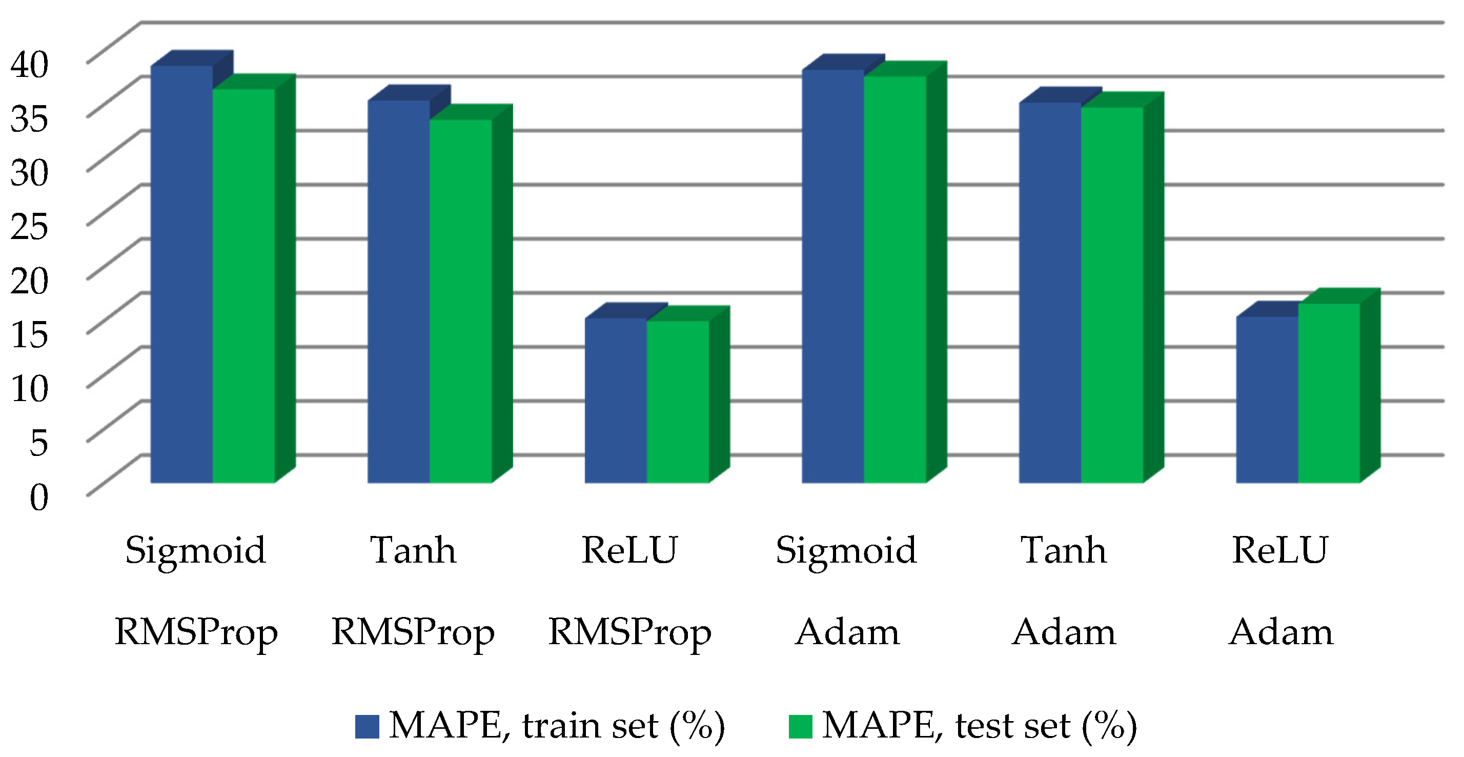
The first step was the choice of a training method. For various activation functions, we applied all the selected training methods. In this case, we used the LSTM as recurrent cells and only L2 regularization (without Dropout). The best results for all the training methods were obtained with the ReLU (
Table 1 and
Figure 3).
RMSProp and Adam significantly outperformed SGD and Momentum, most likely due to the limitation of the oscillations of the neurons’ weights during the training process. Moreover, due to the small size of the model and L2 regularization, the model had low overfitting properties.
We conclude that for the problem under consideration, Adam worked well precisely due to the application of RMSProp learning, not Momentum. Besides, RMSProp compared to Adam is slightly faster because of fewer calculations and less-time-consuming hyper-parameter tuning.
Table 2 and
Figure 4 show the influence of the activation function for two of the best training methods.
In the experiments, the ReLU outperformed Sigmoid and Tanh significantly. The advantage of the ReLU for the DNN and CNN is well known, but our study confirmed that for a small RNN model, the ReLU is also useful because it does not have gradient vanishing problems. Therefore, in the course of the subsequent steps, only the RMSProp with the ReLU was used.
It should be noted that for the LSTM and GRU recurrent cells, we used the default activation functions described in [
30,
31]. For them, replacing the sigmoid function and hyperbolic tangent with ReLU significantly reduced the forecasting accuracy. Additionally, for the output neuron, we used the Logistic Sigmoid function.
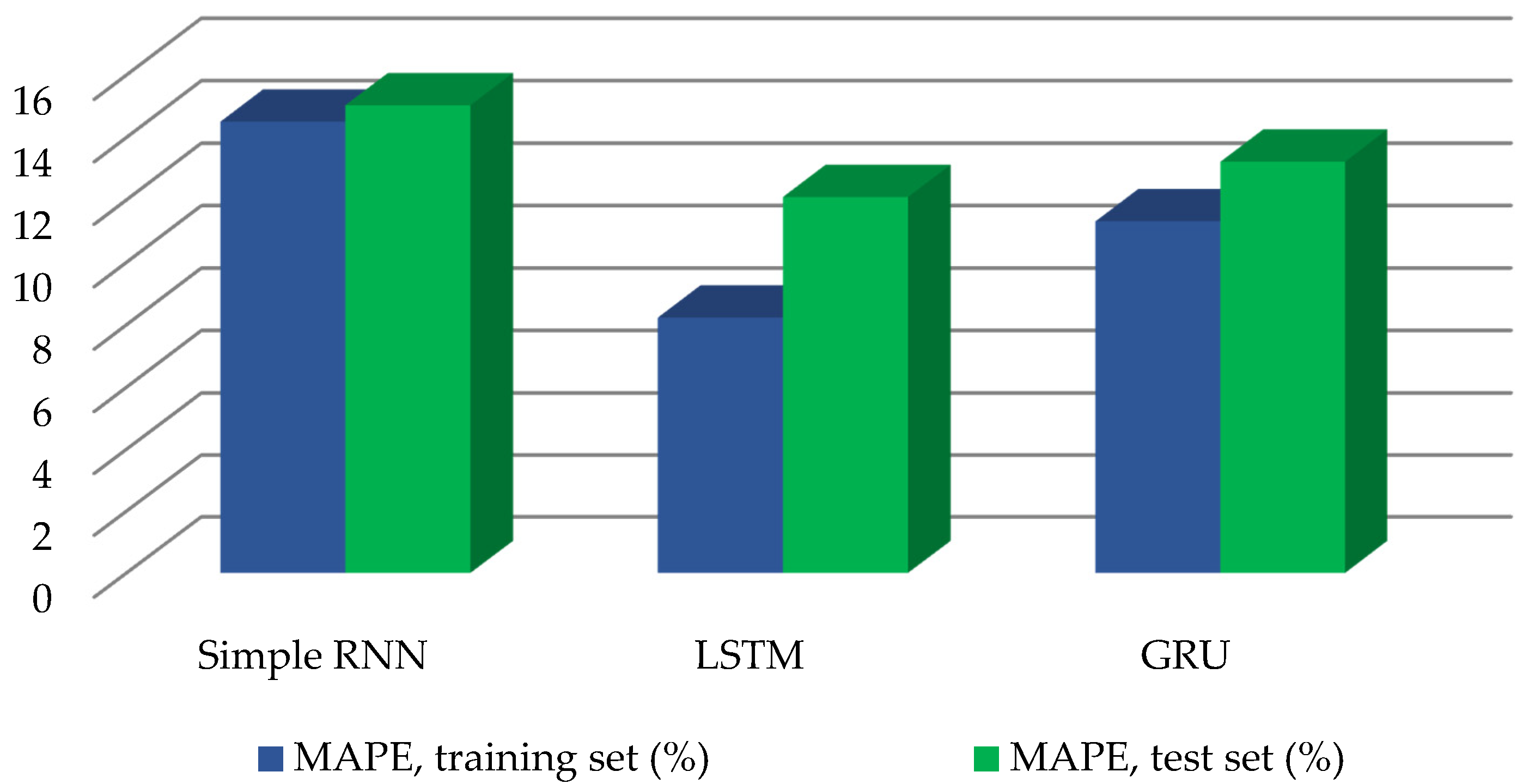
3.4. Type of Recurrent Cells
After choosing the training method and activation functions, we studied the influence of recurrence cells in Layers 3 and 4 (
Figure 1). The results are shown in
Table 3 and
Figure 5.
The type of recurrent cell did not have a substantial effect on the forecasting accuracy compared to the optimization of the training method and activation functions. However, the higher the model accuracy, the more difficult it is to increase the accuracy. Therefore, a continuous decrease in the accuracy difference between the various methods in the course of ANN model tuning is logical. Additionally, if we look at the relative differences in percentages, the application of the LSTM in the test set provided us with 19.6% lower error than SimpleRNN, and GRU, 12% lower error than SimpleRNN.
3.5. Regularization
Overfitting led to the fact that the model found false relations in the training dataset and demonstrated an accuracy on the training data much better than that on the validation and testing data. Initially, in order to eliminate overfitting, we limited the model size and used no more than two recurrent layers and no more than two fully connected (dense) layers.
The robustness and generalization performance are no less important than the forecasting accuracy. If a model can be trained without overfitting and finding false dependencies, it is possible, if necessary, to adapt the model to other data (other conditions). For example, it becomes possible to adjust the model to a different enterprise.
At the same time, the application of a model prone to overfitting carries the risk of a drastic accuracy reduction with even small changes in the technological process of the enterprise. The further training of such models will not provide a significant improvement of the real accuracy since the model will probably find false dependencies again.
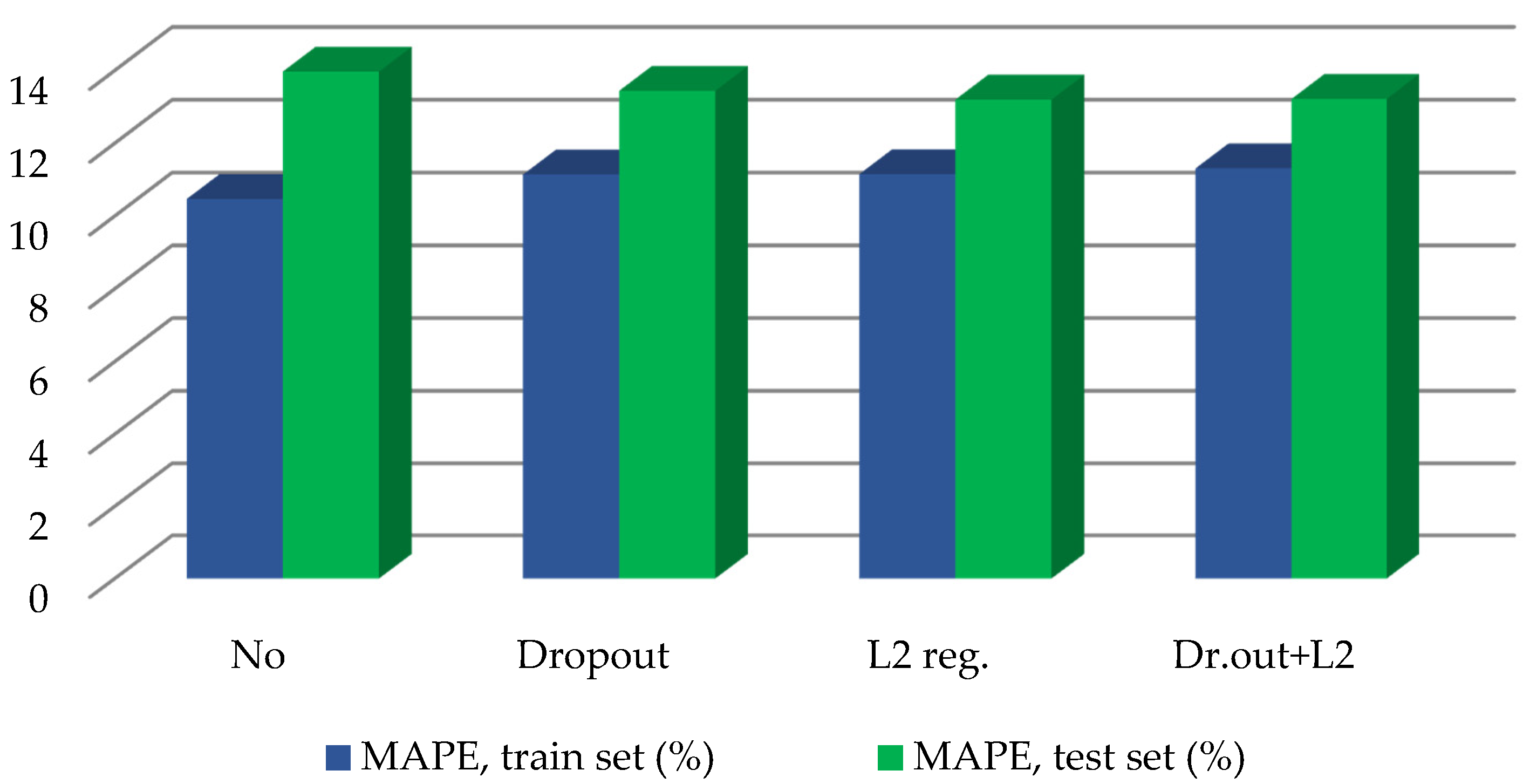
The influence of the Dropout and L2 regularization when using the RMSProp and GRU is detailed in
Table 4 and
Figure 6. The Dropout rate was set to be equal to 0.4; the L2 regularization coefficient was equal to 0.02 or 0.05 depending on the layer (see Lines 4, 5 and 7 of the code and
Figure 1).
During the study, it was proved that it is necessary to apply at least one of the regularization methods to reduce overfitting. Otherwise, the accuracy obtained for the test set is much lower than for the training set. It is better to use both methods since they have different performing mechanisms and influence the varying cases of overfitting.
3.6. Resulting Forecasting Accuracy
Table 5 contains the results of the best configurations of the RNN model developed during the studies. In addition, the RNN architecture was compared with the autoregressive model ARIMA and the simple traditional ANN model, the MLP model. Its hyper-parameters were as follows: numbers of neurons in hidden layers—24, 32, 16 and 1; activation functions in hidden layers—ReLU; L2-regularization coefficient—0.01; Adam training method.
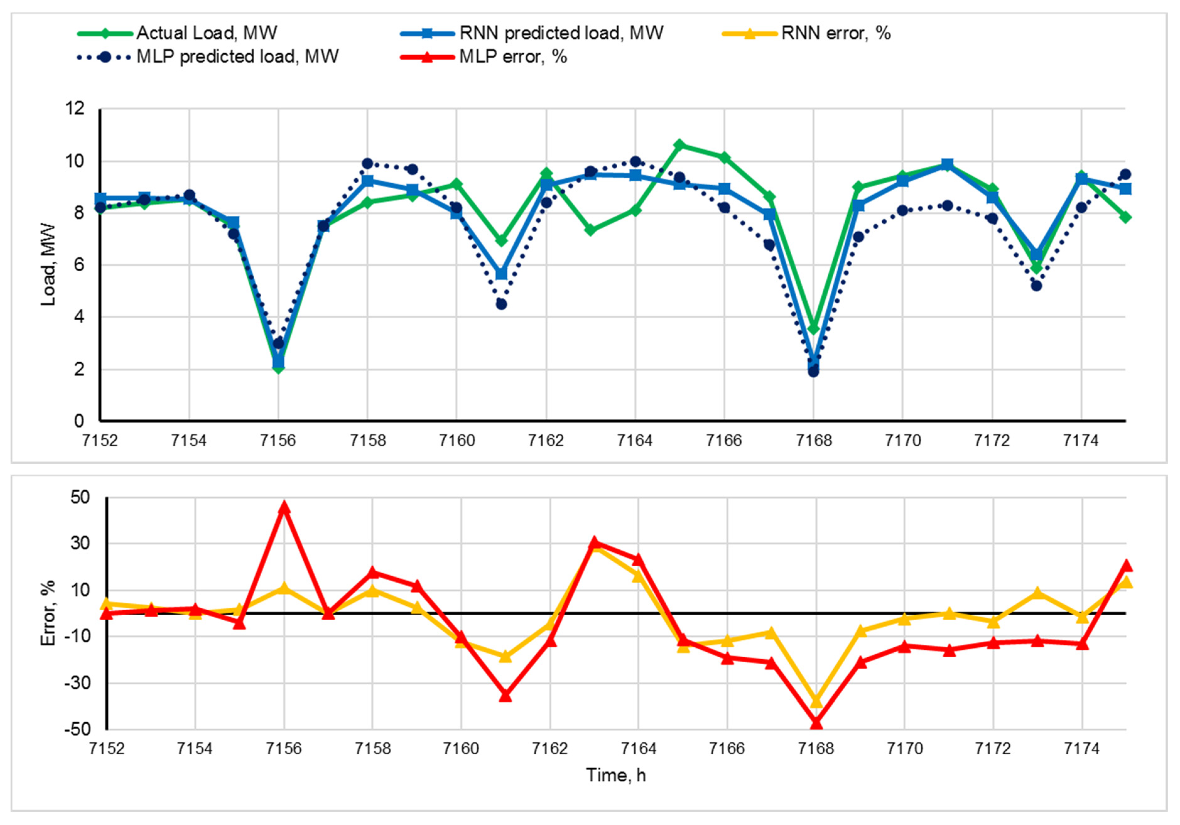
Figure 7,
Figure 8 and
Figure 9 show a comparison of the predicted and the actual loading curves for the daily samples, and
Figure 10 and
Figure 11 show a comparison of the predicted and the actual loading curves for the weekly samples. The resulting RNN model accurately predicted not only the moments but also the magnitudes of the power consumption decrements at the time of shift change (two lowest points on the daily loading curve).
The main reason for the low average accuracy of the forecast is large errors corresponding to the hours when the features of the technological process lead to abrupt variations in the energy consumption schedule. The abrupt variations can be either an increase due to the growth in the coal mining rate or a decrease due to accidents or downtime during blasting.
The computational experiments resulted in the following conclusions about the application of RNNs to this forecasting problem under consideration:
RMSProp and Adam significantly outperformed the SGD and Momentum (see
Table 1 and
Figure 3);
The ReLU activation function in dense layers effectively solves the vanishing gradient problem compared to the Sigmoid function and Hyperbolic tangent (see
Table 2 and
Figure 4);
Recurrent cells with “long memory” such as LSTM and GRU are preferable in comparison with simple recurrent cells; the LSTM-based RNN showed a little higher accuracy but less generalization performance than the GRU-based RNNs (see
Table 3 and
Figure 5);
Even with a small model size, it is necessary to use Dropout and L2 regularization to avoid overfitting (
Table 4 and
Figure 6);
The best configuration in terms of accuracy is RMSProp+LSTM+ReLU. However, the configuration RMSProp+GRU+ReLU is more robust, since it had less bias between the training and test sets. That is why RMSProp+GRU+ReLU was used for the final model design (see
Figure 12).
4. Conclusions
This paper focuses on the application of Recurrent Neural Networks for short-term load forecasting for a coal mining enterprise 48 h ahead. Unlike most industrial consumers with certain daily consumption patterns, the energy consumption of coal mining has a high proportion of irregular processes. The power system of such an enterprise evolves in time and in space. Thus, for the considered problem, the forecasting model is required to be highly robust to adapt to various changes in the technological process.
For this task, the paper proposes a small-size RNN-based model with long memory cells. The small model size allows one to avoid overfitting and to apply a single model for the entire energy consumption schedule, which changes a lot in the course of the enterprise operation and development.
We studied the influence of hyper-parameters and methods of improving the accuracy and generalization performance of the RNN model based on a real-case dataset. The study showed the effectiveness of the RMSProp and Adam training methods. A comparison of the Adam and RMSProp methods was carried out with widely known and easy-to-implement methods: SGD and Momentum. SGD was used as a baseline for comparison, and the use of Momentum helped us to understand that the efficiency of Adam is connected to a greater extent not with the inertia, which is also present in Momentum, but with the variability of the weight gradient, as in RMSProp. This confirms that the considered power consumption is a complex non-stationary process with the presence of rare events that have a significant impact on power consumption.
The effectiveness of the ReLU activation function for dense layers, both LSTM and GRU recurrent cells, and the application of Dropout and (or) L2 regularization were also demonstrated. The resulting MAPE of the load forecasting for 48 h ahead was 11% for the training dataset and 13% for the test dataset.
Thus, the major contribution of the authors to the area of study corresponds to the following main points:
Existing RNN studies consider electric power consumers with a much more periodic schedule and fewer abrupt deviations from the daily average—for example, large buildings’ consumption, joint households and cities. The problem under study is characterized by a high proportion of irregular processes, evolving in time and in space, which have not been addressed in earlier investigations.
Modern research on the neural networks for predicting power consumption uses neural networks (not necessarily recurrent ones) of a very large size. In the presented study, it was shown experimentally that for small RNNs, methods of increasing efficiency such as the ReLU, Adam, RMSProp, Dropout, LSTM and GRU are also applicable.
Comparisons of the LSTM and GRU; the influence of L2-regularization, Dropout and their combination; and a comparison of training methods supported by numerical results for the problem of the short-term load forecasting of industrial enterprises have not been discussed previously. The present study provides a comprehensive understanding of their impact on the accuracy of irregular technological process forecasting.
Within the scope of future work, the RNN model, firstly, will be supplemented with convolution layers for more efficient feature extraction. Secondly, we expect to validate the prediction methodology for different types of industrial customers. Finally, a further comparison with existing methods will also be carried out.

 ,
, 


