Article

A Novel Comparative Statistical and Experimental Modeling of Pressure Field in Free Jumps along the Apron of USBR Type I and II Dissipation Basins

by
Seyed Nasrollah Mousavi
1 and
Daniele Bocchiola
2,*
1
Department of Water Engineering, University of Tabriz, Tabriz 5166616471, Iran
2
Department of Civil and Environmental Engineering, Politecnico di Milano, L. da Vinci, 32, 20133 Milano, Italy
*
Author to whom correspondence should be addressed.
Mathematics 2020, 8(12), 2155; https://doi.org/10.3390/math8122155
Submission received: 7 September 2020 / Revised: 23 November 2020 / Accepted: 29 November 2020 / Published: 3 December 2020
(This article belongs to the Special Issue Applications of Mathematical Models in Engineering)

Abstract

:
Dissipation basins are usually constructed downstream of spillways to dissipate energy, causing large pressure fluctuations underneath hydraulic jumps. Little systematic experimental investigation seems available for the pressure parameters on the bed of the US Department of the Interior, Bureau of Reclamation (USBR) Type II dissipation basins in the literature. We present the results of laboratory-scale experiments, focusing on the statistical modeling of the pressure field at the centerline of the apron along the USBR Type I and II basins. The accuracy of the pressure transducers was ±0.5%. The presence of accessories within basinII reduced the maximum pressure fluctuations by about 45% compared to basinI. Accordingly, in some points, the bottom of basinII did not collide directly with the jet due to the hydraulic jump. As a result, the values of pressure and pressure fluctuations decreased mainly therein. New original best-fit relationships were proposed for the mean pressure, the statistical coefficient of the probability distribution, and the standard deviation of pressure fluctuations to estimate the pressures with different probabilities of occurrence in basinI and basinII. The results could be useful for a more accurate, safe design of the slab thickness, and reduce the operation and maintenance costs of dissipation basins.

1. Introduction

Hydraulic jump with the turbulent entrainment process is a function of time and position. This phenomenon is a complex and stochastic process, so that hydrodynamic pressure fluctuations can be analyzed using statistical methods. Energy dissipation through the hydraulic jumps with the conversion of energy downstream of spillways is usually confined within the dissipation basins [1]. This type of hydraulic structure protects the soil against flow erosion, which can affect the dam’s safety. Due to the large heads upstream of spillways, dissipation basins may be subjected to enormous instantaneous pressure and velocity fluctuations, causing significant stresses in such energy dissipators. This may cause the uplift of a basin lining, making it necessary to provide this structure with sufficient weight or anchorage. Through the analysis of collected data, it is possible to characterize the forces under a hydraulic jump according to the values of mean pressures, pressure fluctuations, and extreme pressures [2].
US Department of the Interior, Bureau of Reclamation (USBR) Type II dissipation basins [3] are designed to reduce excess kinetic energy downstream of the spillway [4,5,6,7,8,9,10], reduce largely (≈30%) the required length compared to smooth basins [11], and help in reducing the costs of the structure [12]. Furthermore, knowledge of the geometric characteristics of the hydraulic jump is fundamental for the design of the dissipation structures. Measurement of fluctuating pressures or forces may be difficult to carry out in the field or at the scale of real structures. Overall, there is a lack of information concerning the hydrodynamic loading on the bottom slabs. Little systematic experimental investigation seems available for Type II dissipation basins, and only a general understanding of the hydraulic behavior is attained [13]. A better understanding of the distribution of pressure fluctuations may lead to a more economical design with high safety of energy dissipation structures.
Toso and Bowers [14] stated that the peak value of the pressure fluctuations intensity coefficient (C′P) varies up to 60% when comparing results from different works. It seems that these differences were related to the degree of development (larger or smaller) of the flow boundary layer. Accordingly, the fully developed flows show lower values of C′P than undeveloped ones. Endres [15] developed a real-time acquisition system and treatment of data representative of the instantaneous pressure fields in a hydraulic jump by analyzing instantaneous pressures downstream of a spillway. Pinheiro [16] measured the pressure fields inside the hydraulic jump downstream of a spillway. He concluded that the pressure fields near the bottom and along the hydraulic jump are lower than the corresponding depth of the mean flow. Marques et al. [17] measured pressures within a dissipation basin with the smooth bed downstream of a spillway. They proposed a dimensionless methodology that groups the fluctuating pressures with different incident Froude numbers (Fr1) in a single trend, being a function of the jump position. The values of Fr1 used by Endres [15], Pinheiro [16], and Marquez et al. [17] were in the range of 4.2 to 8.6, 6 to 10, and 5 to 8, respectively. Based on the pressure data by Enders [15], Teixeira [18] proposed second-order polynomial relationships for estimating different pressure parameters in smooth dissipation basins.
According to Alves [2], the measurement of fluctuating pressures is highly influenced by laboratory conditions. This may include the Reynolds number of flow, transducer accuracy, transducer installation method, hose length, pressure point diameter, channel width, model roughness, etc. Farhoudi et al. [19] studied the pressure fluctuations around some chute blocks in a St. Anthony Fall (SAF) type dissipation basin. Novakoski et al. [20] showed that the negative pressures in the zone near the spillway toe represent the risk of cavitation in the dissipation basin. They concluded that the extreme pressures with the probabilities of occurrence equal to 0.1% and 1% require careful assessment. Macián-Pérez et al. [21] used a numerical model to analyze pressure distributions in a USBR Type II dissipation basin. Hampe et al. [22] estimated extreme pressures in hydraulic jumps with low Froude numbers. Samadi et al. [23] used some explicit data-driven approaches to estimate the C′P coefficient underneath hydraulic jumps on a sloping channel.
Mousavi et al. [24] focused on the minimal and maximal pressures, the pressure coefficients, the power spectral density (PSD), the probability density function (PDF), and the uncertainty analysis of the pressures along a USBR Type I basin (basinI). Mousavi et al. [25] assessed the statistical parameters of free jumps, including mean pressure (P*m), the standard deviation of pressure fluctuations (σ*X), the probability distribution coefficient (NK%), and the pressures with different probabilities (P*K%) along basinI. Mousavi et al. [26] evaluated artificial intelligence models to estimate the C′P coefficient for the free and submerged jumps at the bottom of a USBR Type II basin (basinII). The results showed the deep learning model could estimate the C′P coefficient more accurately.
However, pressure patterns on the apron of basinII have not been widely investigated in the literature. We designed and pursued experiments to obtain some information about the effect of chute blocks and dentated end sill on the free jumps’ characteristics and pressure fluctuation. Experiments were conducted in the centerline of the apron along basinI and basinII with the incident Froude numbers (Fr1) in the range of 6.14 to 8.29. In summary, the differences between the previous works and the present paper are explained as follows:
  • Analysis of the minimal and maximal values of pressures along the free jumps within basinI and basinII. These parameters for basinII have not been investigated in the literature.
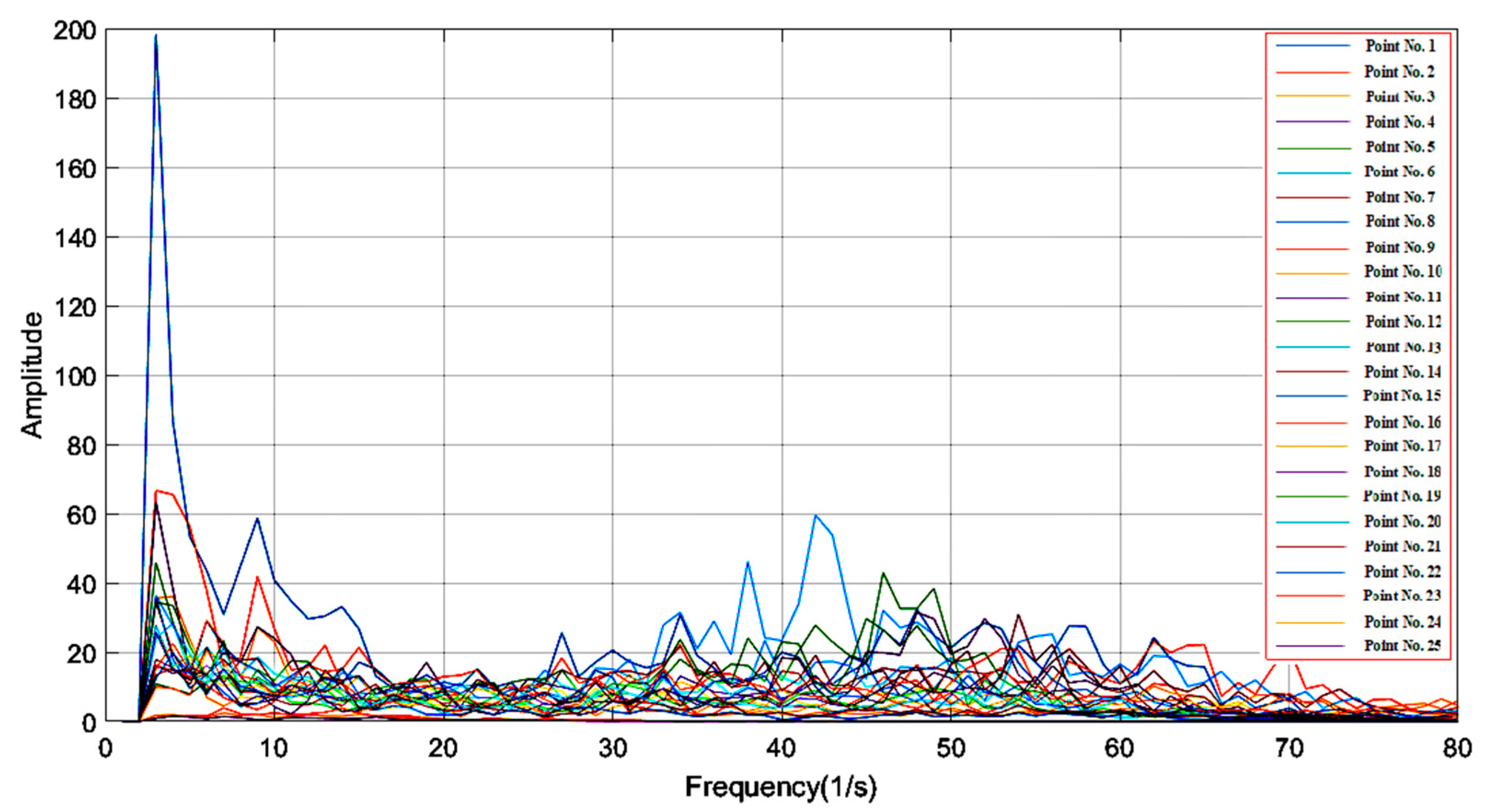
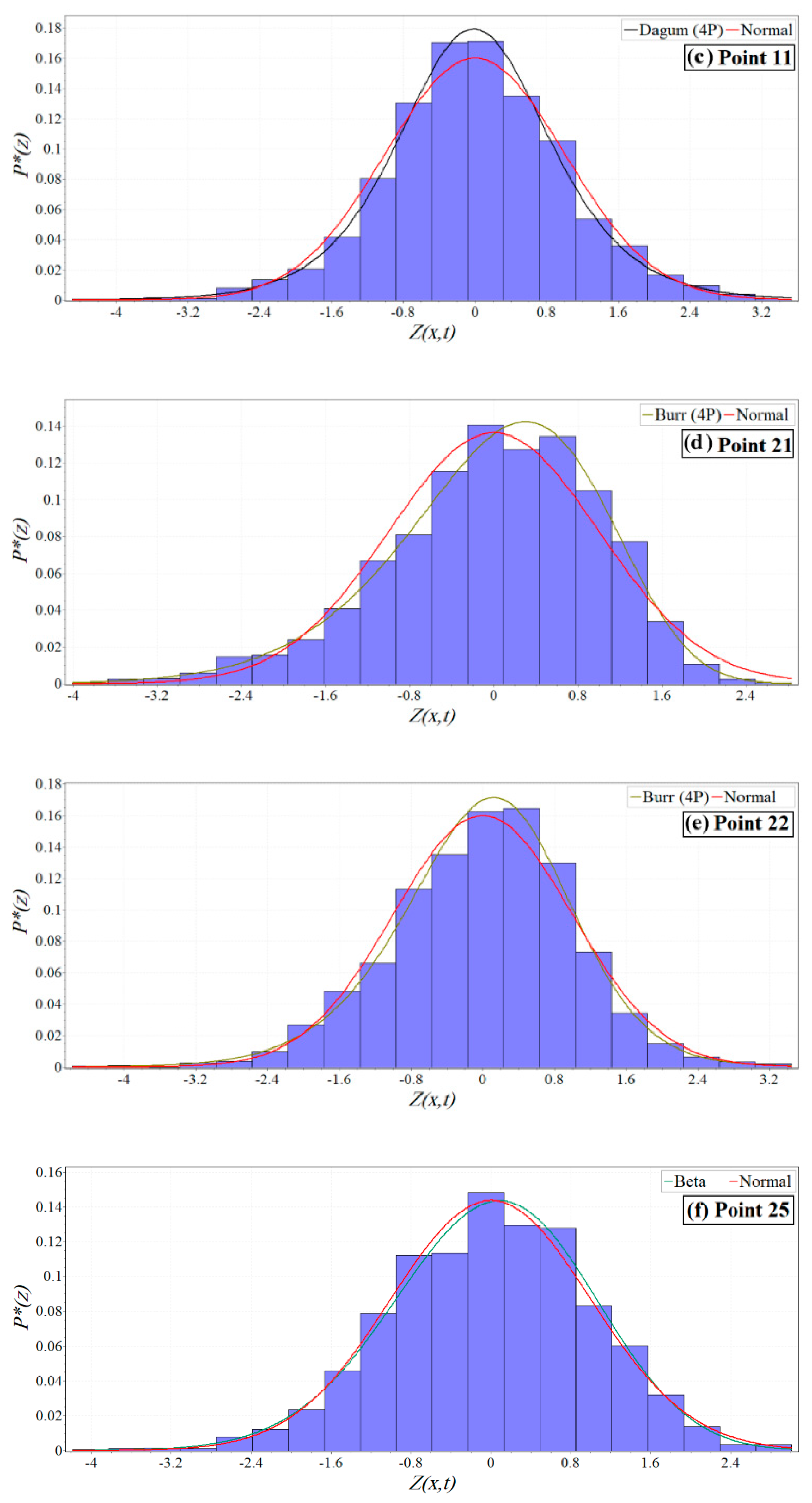
  • Evaluation of the PSD analysis to determine the dominant frequency of fluctuating pressures in the free jumps for basinI and basinII. In addition, assessment of the PDF histograms for the fluctuating pressures at different pressure points and investigation of the skewness and kurtosis coefficients, P*m, extreme pressures (P*min and P*max), σ*X, NK%, and P*K% along basinI and basinII. For reference, we benchmarked and compared our findings with previous similar results of other authors focusing on hydraulic jumps we could retrieve in the present literature.
  • Proposition of some new original best-fit relationships to estimate the dimensionless forms of statistical parameters including P*m, σ*X, NK%, and P*K% for the free jumps as a function of the dimensionless position along basinI and basinII.
  • Proposition of the hydraulic jump length (Lj) as a scaling factor for the dimensionless position from the toe of the spillway (X*). Marques al. [17] proposed the dimensionless adjustments for the pressure parameters. Due to the presence of significant air bubbles at the beginning of the jump, it is difficult to measure the initial depth of the jump (Y1) with great accuracy. It seems that the expression of Y2Y1 (conjugated depths of hydraulic jumps) is not appropriate as a scaling factor. In this case, the X* parameter was defined as X/Lj, where Lj is the length of hydraulic jump. In addition, the values of Y1 were calculated using the well-known equation of Bélanger [27].

2. Materials and Methods

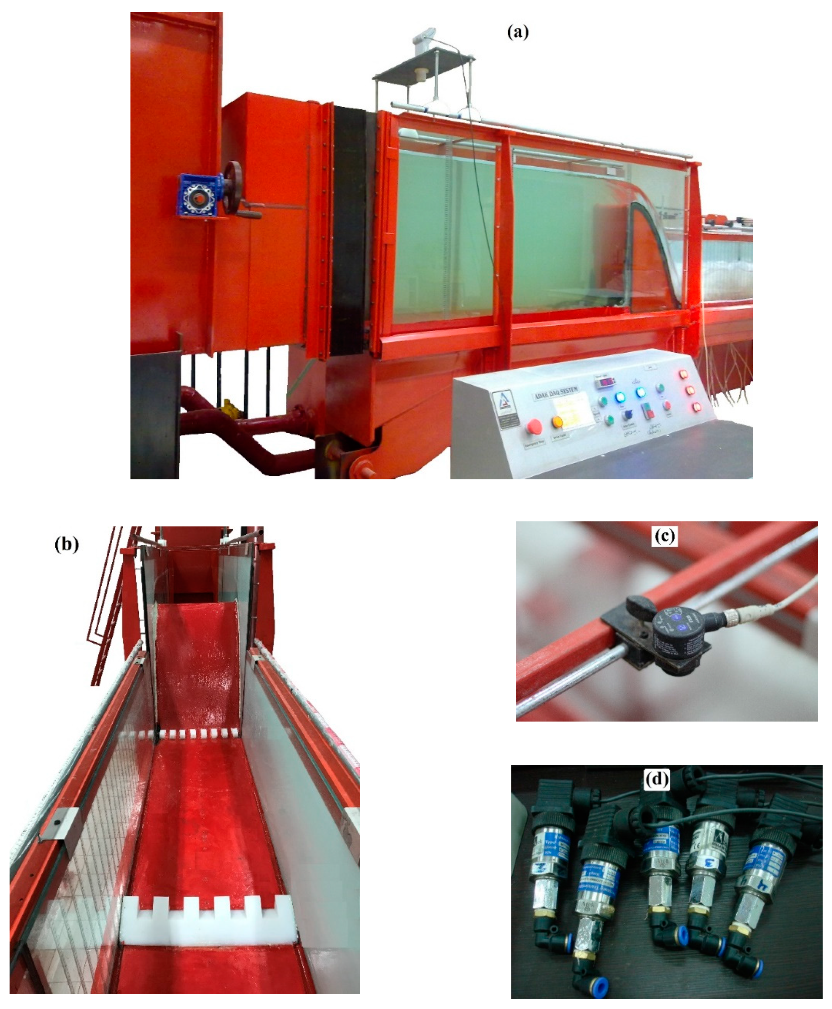
2.1. Experimental Setup

In this research, the pressure field of free jumps was investigated in the hydraulic laboratory, University of Tabriz, Iran (see Figure 1). The laboratory flume used had a length of 10 m, a width of 0.51 m, and a height of 0.5 m. The channel’s bed was considered in the form of a horizontal line in all experiments. An Ogee spillway of 70 cm in height (H) was equipped with two different configurations of the dissipation basins, designed according to the USBR criteria [3]. In addition, the accessories of basinII, including eight chute blocks (3.2 cm width, 3 cm height, and 7.94 cm length) and a dentated end sill with 6 cm height, were designed based on the maximum flow discharge. The spillway was installed at a distance of 260 cm from the entrance head tank of the flume.
We performed some experiments on basinI and basinII with different flow discharges, ranging from 33 to 60.4 L/s, and supercritical Froude numbers (Fr1) between 6.14 and 8.29. According to the USBR recommendation, the lengths of basinI (LI) and basinII (LII) were 200 and 125 cm, respectively. The width of the basins was considered equal to the width of the flume (see Figure 2). At the end of the flume, a hinged weir was used to create and stabilize the free jump position. Therefore, the hydraulic jump was positioned at the basins’ beginning and contained within the basins (i.e., jump type A-jump [28]).
The subcritical flow depth (Y2) at the endpoint of the jumps was measured along the flume’s centerline. To do this, we used a Data logic ultrasonic sensor device model US30, made in Italy with a nominal accuracy of 1 mm. The discharge in the flume (Q) was measured with a transit-time clamp-on ultrasonic flow meter. The values of supercritical flow depth (Y1) were calculated using the Bélanger’s equation [27,29,30], which is defined as follows:
Y 1 Y 2 = 1 2 ( 1 + 1 + 8   Fr 2 2 )
Fr 2 = V 2 g   ×   Y 2
where V2 is the mean subcritical velocity, calculated using the continuity law, Fr2 is the subcritical Froude number, and g is the gravitational acceleration.
To measure the (dynamic) pressure fluctuations, 25 measurement points were considered along the centerline of the apron inside and outside the basinII (see Figure 3). Pressure therein was measured by way of piezometers installed at the centerline of the apron along the basins. The position of the pressure points (X) was from 2.5 cm (piezometer No. 1) to 189 cm (piezometer No. 25). The instantaneous pressures were measured with pressure transducers (Atek BCT 110 series with 100 mbar-A-G1/4 model). The pressure transducers used a 6-channel digital board and have an accuracy of ±0.5% within the range of −1.0 to 1.0 m [24,25,26].
Pressure transducers were calibrated before the experiments using a static pressure gauge in the laboratory. Therefore, the mean fluctuating pressures were approximately equal to the static pressures. The transducers were mounted on a support plate, placed under the bottom of the flume. Thus, it was possible to eliminate possible distortion effects in the pressure signal due to the connection with rubber hoses. The transparent plastic hoses used here had an internal diameter of 3 mm and were 200 cm in length. Hydrodynamic pressure data were measured in time series. Accordingly, some statistical methods were used to analyze the collected pressure data.

2.2. Statistical Parameters

Investigation of the pressure head (cm) parameter is a first step to describe the pressure field in the hydraulic jump. The pressure parameters at each point (PX) include the minimum pressure (Pmin), the mean pressure (Pm), the maximum pressure (Pmax), and the pressure with a certain probability of occurrence (PK%). Marques al. [17] proposed P*X = (PXY1)/(Y2Y1) for the dimensionless form of pressure parameters as a function of the dimensionless position of each point (X*), defined as X* = X/(Y2Y1), where X is the longitudinal position of each point inside the hydraulic jump. As the upstream part of the jump exhibited significant air bubbles, it seems that the scaling of Y2Y1 is not appropriate for the non-dimensional position of the pressure point. As a result, in the present study, the X* parameter was defined as X/Lj, where Lj is the hydraulic jump length.
Knowledge of the extreme pressure heads in the dissipation basins helps to understand the energy dissipation of the hydraulic jumps. In the present study, the extreme pressure heads (P*min and P*max) were investigated in detail. Marques et al. [17] proposed (σ*X/ El) × (Y2/Y1) to analyze the dimensionless standard deviation of the pressure fluctuations at point X. There, El is energy head loss (cm) along the hydraulic jump. The experimental values of PK% were achieved using the pressure time series data collected at each pressure point. The statistical coefficient of the probability distribution (NK%) can be varied at different points of the dissipation basins. Therefore, it is necessary to determine the longitudinal distribution of NK% to estimate the P*K% parameter with a probability to be less than or equal to a certain value (K) along basinI and basinII. As the estimated values of Pm, σX, and NK% were determined at each point inside the basins, the values of PK% can be estimated using equation PK% = Pm + NK% × σ*X [17].
In this study, a new statistical methodology was proposed to estimate the values of P*K% in basinI and basinII. To evaluate the estimated values of pressure parameters, some statistical performance criteria were determined [31,32,33,34]. The PDF function of the normalized pressures along the hydraulic jumps was calculated according to P * ( Z ) = ( 1 / 2 π ) × E x p ( Z 2 / 2 ) . The normalized pressure variable (Z) was defined as ( P [ X , t ] ) P m / σ X , where P[X,t] is the instantaneous pressure [35]. We pursued an analysis of the skewness and kurtosis coefficients of pressure fluctuations [36]. Due to the high variation in S and K coefficients, it is difficult to define a single statistical distribution to describe the overall behavior along the jump.

3. Results and Discussion

3.1. Flow Characteristics

Table 1 presents some experimental and calculated parameters of the flow downstream of the spillway in two dissipation basins under different free jump conditions.
Re1 is the Reynolds number for the supercritical flow of the hydraulic jump. The mean velocity of the incoming flow to the dissipation basins (V1) was computed using the continuity law. According to Table 1, the Y2 parameter in basinII decreases compared to those in the basinI case (classical hydraulic jump). As Q increases, Y1 increases faster than V1. Accordingly, the Froude number reduces when increasing flow discharges. The flow conditions downstream of the spillways are different compared to the sluice gates. The Y1 parameter has an essential role in determining the values of Fr1. Reducing Fr1 with increasing Q for the free jumps downstream of the spillway has been confirmed in previous similar results we were able to retrieve in the present literature [13,17,37,38].

3.2. Power Spectral Density Analysis

The power spectral density (PSD) analysis of the pressure data demonstrates the variation of the PSD parameter in a wide range of frequencies. According to Figure 4, the maximum values of the amplitude corresponding to the dominant frequency decrease by increasing distance from the jump toe. The results indicated that the maximum variation of the PSD parameter in free jumps within basinII was achieved at frequencies less than 5 Hz. It should be noted that the PSD analysis of the fluctuating pressures for different points of basinI with free jumps has been studied by Mousavi et al. [24]. The minimum frequency of pressure transducers is considered to be almost twice the dominant frequency of the signal in the literature [39]. In the present study, a pressure data collection frequency of 20 Hz for 90 s was used for each pressure point. The maximum amplitude at low frequencies along the free jumps indicates large-scale vortices, which is due to the dominance of gravitational forces [40]. Therefore, the Froude law is valid for modeling fluctuating pressures in free jumps.

3.3. Probability Density Function

In this section, the P*(Z) parameter is plotted as a function of the normalized pressure level (Z). Furthermore, the appropriate probability distributions for each pressure point are compared with the normal distribution. The PDF histograms of pressure fluctuations at some points on the bed of basinII in free jumps are shown in Figure 5. In addition, the PDF function of the fluctuating pressures for different points of basinI with the free jumps has been previously investigated by Mousavi et al. [24]. The results indicate that the PDF function does not follow the normal distribution at different points along the free jumps, especially for the initial points of basinII. In other words, the S and K coefficients do not match with the normal distribution values.
According to Fiorotto and Rinaldo [35], positive pressure fluctuations at the beginning of the basins have a relatively high frequency compared to negative pressure fluctuations. In this zone, the S coefficient has positive and maximum values, and the PDF curve tail is drawn to the right. The K values are more than the normal distribution, and the PDF curve is drawn upwards at these points.
At the characteristic point of X*d (point of expected flow detachment), the frequency of positive and negative pressure fluctuations is almost identical, and S ≈ 0 (pressure point No. 11). At this point, pressure values distribution is somewhat similar to the normal distribution. For point No. 21, located at X*r (endpoint of the roller), the S coefficient has negative values. Also, the K coefficient is greater than the normal distribution value. For points located at X*j (endpoint of the hydraulic jump), the S values tend to move towards zero, and the data somewhat follow the normal distribution. Pressure point No. 25 is outside basinII, and it has a normal distribution. The flow energy of the incoming jet is dissipated after passing through the roller point of the jump, and the uniform flow is established almost downstream of the basin. Due to the presence of accessories in basinII, all the considered characteristic points are closer than in the absence of such structures.

3.4. Extreme Pressures

Figure 6 represents variations of the dimensionless minimum, mean, and maximum (scaled) pressures (P*min, P*m, and P*max) as a function of X* in basinII and basinI for different values of Fr1. It is observed that the P*min data reach lower values and have more significant fluctuations concerning the P*m data at the position nearest to the spillway toe (probably due to the incidence of flow in the basin).
The P*min data reach negative values around −0.2 approximately at X* ≤ 0.20 for basinII, and of −0.4 at X* ≤ 0.30 for basinI, increasing with oscillations after that. This may indicate zones subject to low pressure, which may be associated with erosion or cavitation processes. Therefore, basinII is more reliable than basinI in terms of the possibility of cavitation. At the position of X*j, P*min data begin to oscillate near the value 1.0 and slightly lower. Concerning the values of P*max, the higher and more disparate values versus the P*m values occur near the spillway, caused by the direct impact of the flow jet on the dissipation basins. The values of extreme pressures in basinII are lower than those for basinI. There is a narrower pressure range in basinII compared to basinI. The results indicate that P*max seemingly decreases with the increasing Froude number, with P*m and P*min somewhat constant, in the explored range. Using the results obtained in the present study by adjusting the values of P*X, including P*min, P*m, and P*max, a new second-order rational expression was developed for basinII and basinI. Equation (3) is valid for 0 < X* ≤ 1.85 in basinII and 0 < X* ≤ 1.30 in basinI. According to Figure 6, one can estimate P*X using Equation (3). The values of α, β, γ, and δ to estimate P*X for basinII and basinI are provided in Table 2.
P X * = α + β   X * 1 + γ   X * + δ   X * 2

3.5. Standard Deviation of Fluctuating Pressures

The σ*X parameter is a function of the flow discharge and the pressure point position relative to the beginning of the jump. In Figure 7, increasing flow discharge (i.e., decreasing Froude number) results in σ*X increasing. As Q increases, the dynamic energy increases, and the fluctuating component of pressure (P′) increases as well, indicating the turbulence intensity of the flow. Along the jump, σ*X increases to a maximum value, in the range of X* ≤ 0.33 for basinI and basinII, and decreases after that. It seems that the main factors for the fluctuations of pressures along the jump are turbulent flow, eddies formation, and their movement during the jump. Therefore, in some positions, the interaction of eddies and the basin bed causes a sudden increase in the bed pressure.
Figure 7b shows a comparison of the σ*X values in the case of basinI with the results obtained by Pinheiro [16] and Marques et al. [17] for free jumps. It is seen that our study displays similar patterns to their work. However, in the downstream zone of the basin, σ*X values are relatively higher than the results obtained by others. This is likely to be linked to the determination of Y1 and Y2 and identification of the initial position of the hydraulic jump. The σ*X values for the smooth bed (basinI) are greater than in basinII with blocks. Accordingly, the presence of accessories within the hydraulic jumps significantly decreases σ*X. Figure 7 demonstrates the values of σ*X max for different Froude numbers in basinII and basinI. A high value of σ*X max may indicate a considerable variation of the dynamic pressures on the bottom slab, damaging the structure. According to Figure 7, as the Froude number (Fr1) increases, the intensity of pressure fluctuations decreases. According to Teixeira [18], the average value of σ*X max in a smooth basin was about 0.7.
As seen in Table 3, one has σ*X max ≈ 0.50~0.68 for basinII, and σ*X max ≈ 1.02~1.20 for basinI, similarly for all Froude numbers. Accordingly, the values of σ*X max in basinII decreased down to about −45% compared with basinI for the free jumps. The X*σmax position in the presence of the blocks and end sill is closer to the spillway toe. The accessories on the bed of basinII may cause the jet to be spread or submerged. Due to the presence of chute blocks at some points, the bottom of basinII does not collide directly with the jet due to the hydraulic jump. Consequently, the values of pressure and pressure fluctuations decrease mainly therein. Figure 7 illustrates the σ*X values for different Froude numbers in basinI and basinII.
We optimized Teixeira’s method [18] to assess σ*X for basinII and basinI. A new second-order rational expression was developed in the range of 0 < X* ≤ 1.85 for basinII and 0 < X* ≤ 1.30 for basinI. According to Figure 7, one can estimate σ*X using Equation (4). The values of a, b, c, and d to determine σ*X are provided in Table 4.
σ X * = a + b   X * 1 + c   X * + d   X * 2
Therefore, the new adjustment can estimate σ*X very well with a correlation coefficient (R) equal to 0.910 and 0.872 for basinII and basinI, respectively.

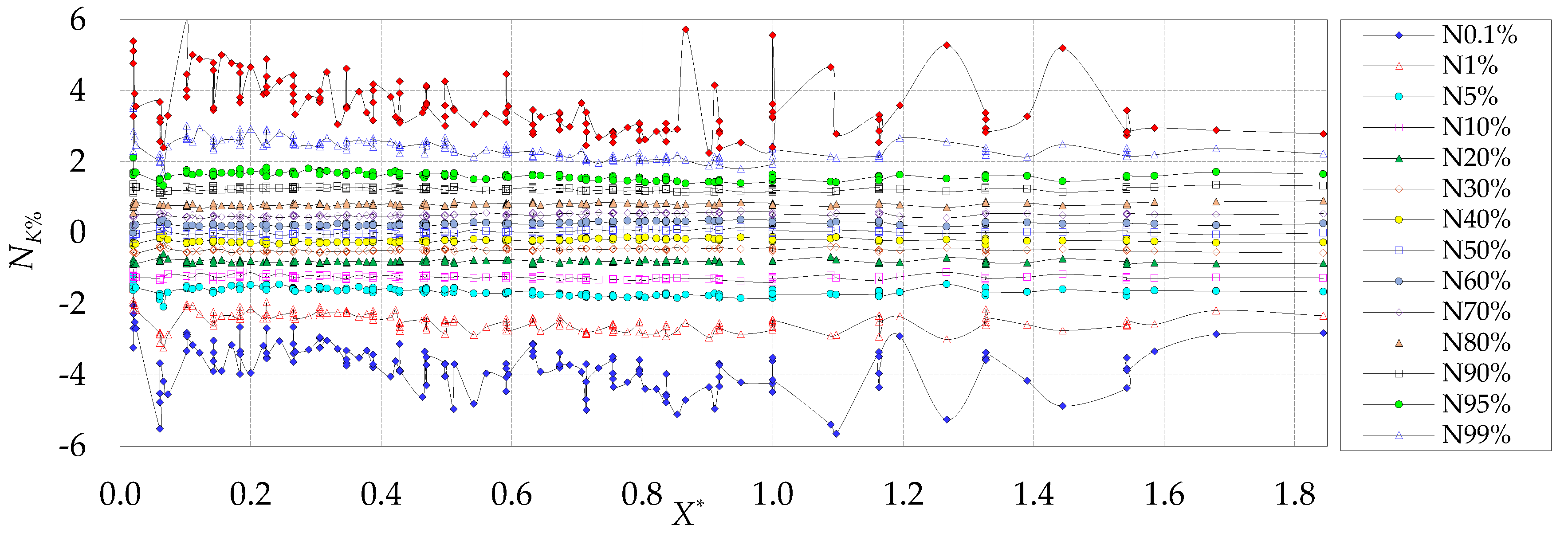
3.6. Statistical Coefficient of the Probability Distribution

Figure 8 presents the distribution of the experimental values of the NK% coefficient obtained from the pressure data along basinII for different probabilities from 0.1% to 99.9% with different flow conditions in free jumps. The distribution of the NK% coefficient along basinI with the free jumps has been previously investigated by Mousavi et al. [25].
From Figure 8, one can verify the dispersion of the NK% coefficient with the minimum and maximum extreme pressures in the initial zone of the jumps. It is observed that for probabilities greater than 50%, the NK% coefficient has positive values, and for probabilities less than 50%, it has negative values. At the beginning area of the basins, the values of N0.1% are approximately −3, and for positions X* ≥ 0.40, it has values less than −4. In addition, the N99.9% coefficient at the beginning of basinII has values around 4 to 6. At the downstream of the basins, the NK% values are slightly stabilized and vary in the range of 2 to 4. The results show that the variation rate of the NK% coefficient along basinII has decreased somewhat compared to basinI.
Teixeira [18] demonstrated that in free jumps, the longitudinal distribution of the NK% coefficient follows a second-order polynomial relationship. In the present study, the results show that the NK% coefficient has relatively constant values along the jumps, mainly for the probabilities from 5% to 95%. Accordingly, depending on the probability to be identified, the NK% coefficient shows a trend more or less close to a single (average) value for each probability, regardless of Fr1 values. Table 5 displays the average experimental values of the NK% coefficient with different probabilities along the basins.
To develop a method for estimating the P*K% parameter in the case of basinII and basinI, we identified variations in the NK% coefficient as a function of probability. Therefore, it was decided to use the average value of NK% for each probability. According to Wiest [41], there is little effect of Fr1 on NK%, and the latter remains constant along the dissipation basin. Accordingly, NK% follows a specific curve acceptably well, making it possible to establish a new adjustment for NK% as a function of the probability of occurrence (K). Therefore, we propose a second-order rational relationship to estimate NK%:
N K % = α + β   K 1 + γ   K + δ   K 2
Here α, β, γ, and δ are the coefficients of Equation (5), and K is the value of the probability in decimal. The values of coefficients in Equation (5) are shown in Table 6. The residual of the experimental and estimated data set of the NK% coefficient for different probabilities in basinII and basinI is plotted in Figure 9. This parameter is defined as the difference between the experimental and estimated values of NK%.

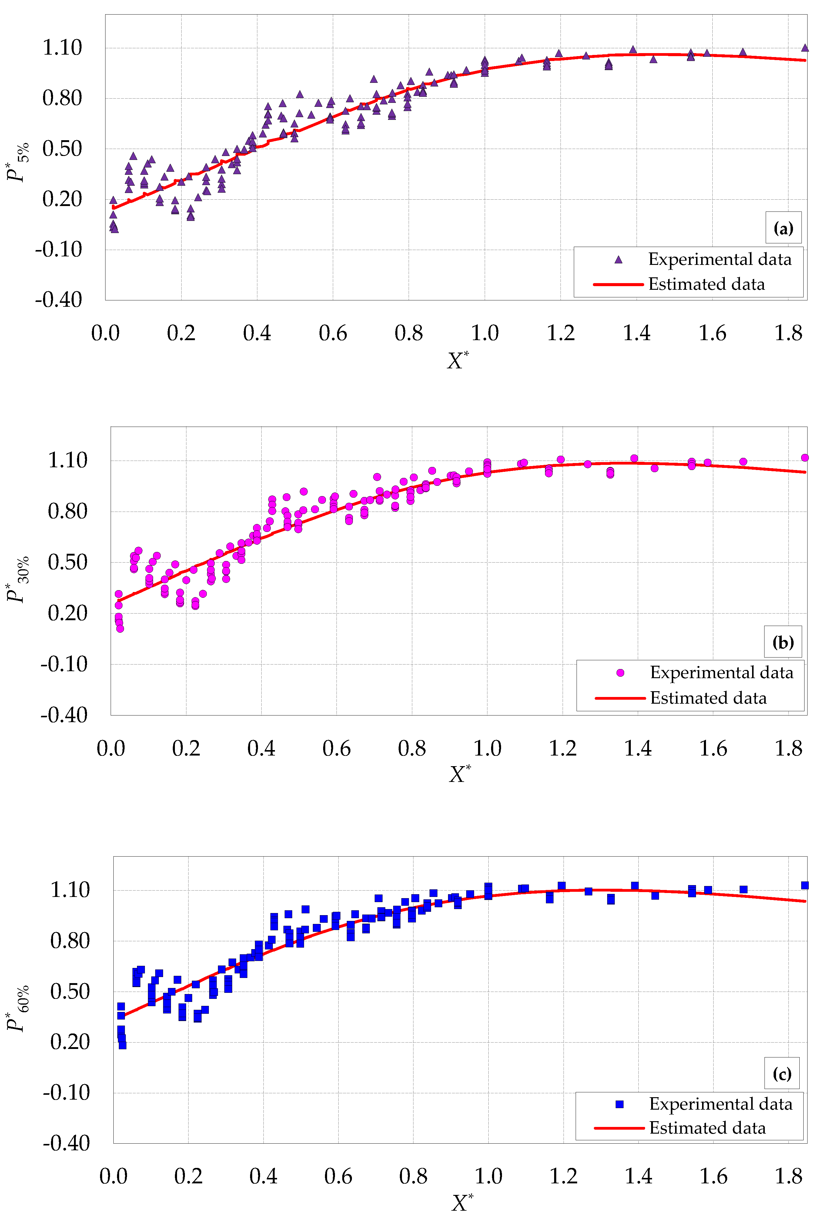
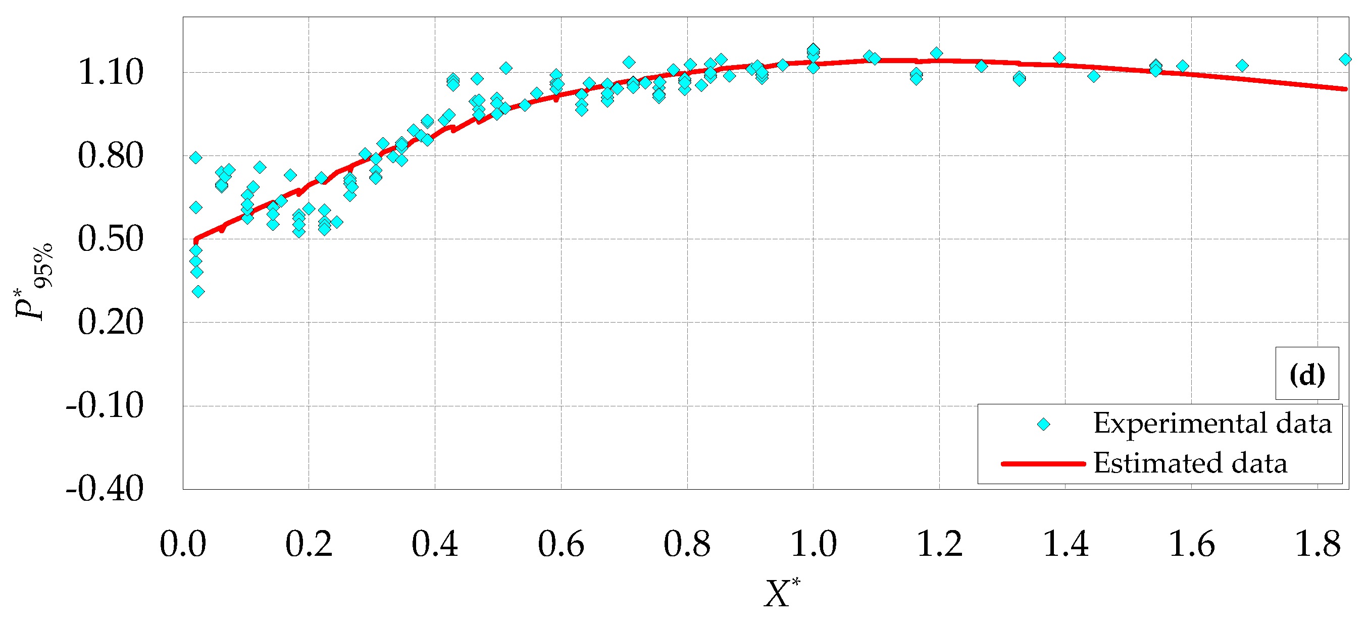
3.7. Estimation of Pressures with Different Probabilities of Occurrence

In this study, new original adjustments were proposed for P*m (Equation (3)), σ*X (Equation (4)), and NK% (Equation (5)) to estimate the pressure values with different probabilities of occurrence (PK%). Therefore, the estimated values of Pα% were determined using Equation Pα% = Pm + NK% × σX.
Some statistical criteria for the estimated values of the P*K% parameter in basinII and basinI are presented in Table 7. For instance, the longitudinal distribution of the experimental and estimated data of the P*K% parameter with different probabilities along basinII is shown in Figure 10. The distribution of the P*K% parameter for different probabilities of occurrence along basinI with the free jumps has been previously investigated by Mousavi et al. [25].

4. Conclusions

In this study, a lab-scale model of an Ogee spillway, either equipped with the USBR Type I and II dissipation basins was installed downstream of an Ogee spillway, based on the USBR criteria, to investigate pressure fields therein. The present study aimed to measure and provide useful insights about the pressure fluctuations at the bottom of basinII. We can provide here some conclusions from our research, covering the (different) patterns of pressures along the free hydraulic jumps, as follows:
(i)
For the first time to our knowledge, our results allow calculation of the statistics and extreme values of the pressure field occurring on the bed of the dissipation basins, and demonstrate the advantage of using a USBR Type II basin in terms of reduced stress over the basin’s bed.
(ii)
The Y2 parameter in basinII was decreased against that in basinI. In addition, with increasing flow discharge (Q), supercritical flow depth (Y1) increased more than velocity (V1). As a result, Fr1 reduced with higher Q values.
(iii)
The P*min data reached negative values of around −0.2 approximately at X* ≤ 0.2 for basinII, and of −0.4 at X* ≤ 0.3 for basinI (i.e., very close to spillway toe). Therefore, basinII was more reliable than basinI in terms of the possibility of cavitation. More fluctuating values of P*max against the mean values occurred near the spillway, justified by the direct impact of the flow jet on the dissipation basin.
(iv)
Analysis of σ*X showed that the dimensionless position of X*σmax is close to 0.20 and 0.29 for basinII and basinI, respectively, with pressure fluctuations decreasing after that. Accordingly, the position of X*σmax was closer to the spillway toe for basinII. With increasing flow discharge, the pressure fluctuations increased. The pressure fluctuations range on the basin bed was visibly narrower for basinII than for basinI. For basinII, σ*Xmax values along the free jumps were reduced by −40% compared to basinI.
(v)
Based on the methodologies proposed by Marques et al. [17] and Teixeira [18], new original best-fit adjustments were proposed here for the P*m, σ*X, and NK% parameters to estimate the P*K% parameter in the case of basinI and basinII. In addition, we originally displayed that NK% values show a trend towards a single average value independently of the Froude number, and we proposed an adjustment for NK% as a function of probability.
(vi)
Some effort may be devoted to investigating the statistical distribution of pressures on the basin bed. As observed, a deviation of the skewness from the S = 0 value for normal distribution in the beginning area of the basins indicates a different and asymmetric distribution. Positively skewed distributions indicate the potential for more (than normally expected) frequent outbursts of large flow pressure, possibly requiring the increase of the structural resistance of the basin apron.
(vii)
The laboratory-scale models presented herein have several limitations that should guide further research on the topic. It should be noted that there is a potential error in scaling the pressure heads. Therefore, just indicating the dimensionless terms may be misleading.
(viii)
The results of this work contribute to the present debate about the use of dissipation basins, and especially of USBR Type II ones for spillway flow calming, providing a quantitative assessment of some main features of the hydraulic jump within the dissipation basin, and the modified (reduced) maximum pressure on the basin apron, and are potentially useful for designing dissipation basins in real-world applications.

Author Contributions

Methodology, S.N.M. and D.B.; validation, D.B.; writing—original draft, S.N.M.; writing—review and editing, D.B. Both authors have read and agreed to the published version of the manuscript.

Funding

This research received no external funding.

Acknowledgments

All co-authors would like to express their gratitude to the editors and reviewers for their time spent reviewing our manuscript and for helping to improve the manuscript. Daniele Bocchiola acknowledges the support from the Climate-Lab of the Polytechnic University of Milan (https://www.climatelab.polimi.it/en/), an interdepartmental laboratory on climate change at the Polytechnic University of Milan.

Conflicts of Interest

The authors declare no conflict of interest.

Abbreviation

The following symbols are used in this paper:
BBasin width (L)
basinIUSBR Type I dissipation basin
basinIIUSBR Type II dissipation basin
C′PPressure fluctuations intensity coefficient
ElEnergy head loss along the hydraulic jump (L)
Fr1Supercritical Froude number
Fr2Subcritical Froude number
gGravitational acceleration (LT−2)
HOgee spillway height
KKurtosis coefficient
LILength of basinI (L)
LIILength of basinII (L)
LjLength of hydraulic jump (L)
MAEMean absolute error
NK%Statistical coefficient of the probability distribution
PK%Pressure head with a certain probability of occurrence (L)
PminMinimum extreme pressure (L)
PmMean pressure head at each pressure point (L)
PmaxMaximum extreme pressure (L)
PSDPower spectral density of the pressure data
P(X,t)Instantaneous pressure (L)
P*ZProbability density function (PDF) of the normalized fluctuating pressures
P′Fluctuating component of pressure (L)
QFlow discharge (L3T−1)
RCorrelation coefficient
Re1Reynolds number for the supercritical flow of the hydraulic jump
RMSERoot mean squared error
SSkewness coefficient
USBRUS Department of the Interior, Bureau of Reclamation
V1Mean velocity of the coming flow to the dissipation basin (LT−1)
V2Mean subcritical velocity (LT−1)
WIWillmott’s index of agreement
XLongitudinal position of each point inside the hydraulic jump (L)
X*Dimensionless position of each point (X/Lj)
X*dCharacteristic point of the expected flow detachment
X*rCharacteristic endpoint of the roller
X*jCharacteristic endpoint of the hydraulic jump
Y1Supercritical flow depth at the jump toe (L)
Y2Subcritical flow depth at the end of the jump (L)
ZNormalized pressure variable
σXStandard deviation of the pressure fluctuations at point X (L)
σ*XDimensionless standard deviation of the pressure fluctuations at point X (L)
1Supercritical flow
2Subcritical flow
mMean value
maxMaximum value
minMinimum value
*Dimensionless value

References

  1. Khatsuria, R.M. Hydraulics of Spillways and Energy Dissipators; Marcel Dekker: New York, NY, USA, 2005. [Google Scholar]
  2. Alves, A.A.M. Characterization of Hydrodynamic Forces in Dissipation Basins under Hydraulic Jumps with Low Froude Number; Universidade Federal do Rio Grande do Sul: Porto Alegre, Brazil, 2008. (In Portuguese) [Google Scholar]
  3. USBR. Spillways. In Design of Small Dams, 3rd ed.; US Department of the Interior, Bureau of Reclamation: Washington, DC, USA, 1987; pp. 339–437. [Google Scholar]
  4. Mohamed Ali, H. Effect of roughened-bed stilling basin on length of rectangular hydraulic jump. J. Hydraul. Eng. 1991, 117, 83–93. [Google Scholar] [CrossRef]
  5. Verma, D.; Goel, A. Stilling basins for pipe outlets using wedge-shaped splitter block. J. Irrig. Drain. Eng. 2000, 126, 179–184. [Google Scholar] [CrossRef]
  6. Alikhani, A.; Behrozi-Rad, R.; Fathi-Moghadam, M. Hydraulic jump in stilling basin with vertical end sill. Int. J. Phys. Sci. 2010, 5, 25–29. [Google Scholar]
  7. Tiwari, H.; Goel, A.; Gahlot, V. Experimental Study of effect of end sill on stilling basin performance. Int. J. Eng. Sci. Technol. 2011, 3, 3134–3140. [Google Scholar]
  8. Cancian Putton, V.; Marson, C.; Fiorotto, V.; Caroni, E. Supercritical flow over a dentated sill. J. Hydraul. Eng. 2011, 137, 1019–1026. [Google Scholar] [CrossRef]
  9. Tiwari, H.; Goel, A. Effect of end sill in the performance of stilling basin models. Am. J. Civil Eng. Archit. 2014, 2, 60–63. [Google Scholar] [CrossRef] [Green Version]
  10. Fecarotta, O.; Carravetta, A.; Del Giudice, G.; Padulano, R.; Brasca, A.; Pontillo, M. Experimental results on the physical model of an USBR type II stilling basin. In Proceedings of the River Flow 2016, International Conference on Fluvial Hydraulics, St. Louis, MI, USA, 10–14 July 2016. [Google Scholar]
  11. Chanson, H.; Carvalho, R. Hydraulic jumps and stilling basins. In Energy Dissipation in Hydraulic Structures; Chanson, H., Ed.; CRC Press: Leiden, The Netherlands, 2015; pp. 65–104. [Google Scholar]
  12. Vischer, D.; Hager, W.H. Dam Hydraulics; Wiley: Ürich, Switzerland, 1998; Volume 2. [Google Scholar]
  13. Padulano, R.; Fecarotta, O.; Del Giudice, G.; Carravetta, A. Hydraulic design of a USBR Type II stilling basin. J. Irrig. Drain. Eng. 2017, 143, 1–9. [Google Scholar] [CrossRef] [Green Version]
  14. Toso, J.W.; Bowers, C.E. Extreme pressures in hydraulic-jump stilling basins. J. Hydraul. Eng. 1988, 114, 829–843. [Google Scholar] [CrossRef]
  15. Endres, L.A.M. Contribution to the Development of a System for the Acquisition and Processing of Instantaneous Pressures Data in the Laboratory; Federal University of Rio Grande do Sul: Porto Alegre, Brazil, 1990. (In Portuguese) [Google Scholar]
  16. Pinheiro, A.A.d.N. Hydrodynamic Actions in Thresholds for Energy Dissipation Basin by Hydraulic Jumps; Universidade Técnica de Lisboa: Lisbon, Portugal, 1995. (In Portuguese) [Google Scholar]
  17. Marques, M.G.; Drapeau, J.; Verrette, J.-L. Pressure fluctuation coefficient in a hydraulic jump. Braz. J. Water Resour. (Rbrh) 1997, 2, 45–52. (In Portuguese) [Google Scholar]
  18. Teixeira, E.D. Scale Effect on Estimating Extreme Pressure Values on the Bed of the Hydraulic Dissipation Basins; Universidade Federal do Rio Grande do Sul: Porto Alegre, Brazil, 2008. (In Portuguese) [Google Scholar]
  19. Farhoudi, J.; Sadat-Helbar, S.; Aziz, N.I. Pressure fluctuation around chute blocks of SAF stilling basins. J. Agric. Sci. Technol. 2010, 12, 203–212. [Google Scholar]
  20. Novakoski, C.K.; Hampe, R.F.; Conterato, E.; Marques, M.G.; Teixeira, E.D. Longitudinal distribution of extreme pressures in a hydraulic jump downstream of a stepped spillway. Braz. J. Water Resour. (Rbrh) 2017, 22. [Google Scholar] [CrossRef] [Green Version]
  21. Macián-Pérez, J.F.; García-Bartual, R.; Huber, B.; Bayon, A.; Vallés-Morán, F.J. Analysis of the flow in a typified USBR II stilling basin through a numerical and physical modeling approach. Water 2020, 12, 227. [Google Scholar] [CrossRef] [Green Version]
  22. Hampe, R.F.; Steinke Júnior, R.; Prá, M.D.; Marques, M.G.; Teixeira, E.D. Extreme pressure forecasting methodology for the hydraulic jump downstream of a low head spillway. Braz. J. Water Resour. (Rbrh) 2020, 25, 1–10. [Google Scholar] [CrossRef] [Green Version]
  23. Samadi, M.; Sarkardeh, H.; Jabbari, E. Explicit data-driven models for prediction of pressure fluctuations occur during turbulent flows on sloping channels. Stoch. Environ. Res. Risk Assess. 2020, 34, 691–707. [Google Scholar] [CrossRef]
  24. Mousavi, S.N.; Farsadizadeh, D.; Salmasi, F.; Dalir, A.H.; Bocchiola, D. Analysis of minimal and maximal pressures, uncertainty and spectral density of fluctuating pressures beneath classical hydraulic jumps. Water Supply 2020, 20, 1909–1921. [Google Scholar] [CrossRef]
  25. Mousavi, S.N.; Júnior, R.S.; Teixeira, E.D.; Bocchiola, D.; Nabipour, N.; Mosavi, A.; Shamshirband, S. Predictive modeling the free hydraulic jumps pressure through advanced statistical methods. Mathematics 2020, 8, 323. [Google Scholar] [CrossRef] [Green Version]
  26. Mousavi, S.N.; Farsadizadeh, D.; Salmasi, F.; Hosseinzadeh Dalir, A. Evaluation of pressure fluctuations coefficient along the USBR Type II stilling basin using experimental results and AI models. ISH J. Hydraul. Eng. 2020. [Google Scholar] [CrossRef]
  27. Belanger, J.B. Essay on the Numerical Solution of Some Problems Related to the Constant Motion of Water Flow; Carilian-Goeury: Paris, France, 1828. (In French) [Google Scholar]
  28. Hager, W.H.; Li, D. Sill-controlled energy dissipator. J. Hydraul. Res. 1992, 30, 165–181. [Google Scholar] [CrossRef]
  29. Chaudhry, M.H. Open-Channel Flow, 2nd ed.; Springer Science & Business Media: New York, NY, USA, 2008. [Google Scholar]
  30. Chanson, H. Development of the Bélanger equation and backwater equation by Jean-Baptiste Bélanger (1828). J. Hydraul. Eng. 2009, 135, 159–163. [Google Scholar] [CrossRef] [Green Version]
  31. Bennett, N.D.; Croke, B.F.; Guariso, G.; Guillaume, J.H.; Hamilton, S.H.; Jakeman, A.J.; Marsili-Libelli, S.; Newham, L.T.; Norton, J.P.; Perrin, C. Characterising performance of environmental models. Environ. Model. Softw. 2013, 40, 1–20. [Google Scholar] [CrossRef]
  32. Willmott, C.J.; Matsuura, K. Advantages of the mean absolute error (MAE) over the root mean square error (RMSE) in assessing average model performance. Clim. Res. 2005, 30, 79–82. [Google Scholar] [CrossRef]
  33. Chai, T.; Draxler, R.R. Root mean square error (RMSE) or mean absolute error (MAE)?–Arguments against avoiding RMSE in the literature. Geosci. Model Dev. 2014, 7, 1247–1250. [Google Scholar] [CrossRef] [Green Version]
  34. Willmott, C.J.; Robeson, S.M.; Matsuura, K. A refined index of model performance. Int. J. Climatol. 2012, 32, 2088–2094. [Google Scholar] [CrossRef]
  35. Fiorotto, V.; Rinaldo, A. Turbulent pressure fluctuations under hydraulic jumps. J. Hydraul. Res. 1992, 30, 499–520. [Google Scholar] [CrossRef]
  36. Sharma, C.; Ojha, C. Statistical parameters of hydrometeorological variables: Standard deviation, SNR, skewness and kurtosis. In Advances in Water Resources Engineering and Management; Springer: Singapore, 2020; Volume 39, pp. 59–70. [Google Scholar]
  37. Novakoski, C.K.; Conterato, E.; Marques, M.; Teixeira, E.D.; Lima, G.A.; Mees, A. Macro-turbulent characteristcs of pressures in hydraulic jump formed downstream of a stepped spillway. Braz. J. Water Resour. (Rbrh) 2017, 22. [Google Scholar] [CrossRef] [Green Version]
  38. Prá, M.D.; Priebe, P.d.S.; Teixeira, E.D.; Marques, M.G. Evaluation of pressure fluctuation in hydraulic jump by dissociation of hydraulic forces. Braz. J. Water Resour. (Rbrh) 2016, 21, 221–231. (In Portuguese) [Google Scholar]
  39. Yan, Z.-M.; Zhou, C.-T.; Lu, S.-Q. Pressure fluctuations beneath spatial hydraulic jumps. J. Hydrodyn. 2006, 18, 723–726. [Google Scholar] [CrossRef]
  40. Pei-Qing, L.; Ai-Hua, L. Model discussion of pressure fluctuations propagation within lining slab joints in stilling basins. J. Hydraul. Eng. 2007, 133, 618–624. [Google Scholar] [CrossRef]
  41. Wiest, R.A. Evaluation of the Pressure Field in Hydraulic Jump Formed Downstream of a Spillway with Different Submergence Degrees; Universidade Federal do Rio Grande do Sul: Porto Alegre, Brazil, 2008. (In Portuguese) [Google Scholar]
Figure 1. Laboratory flume and experimental setup. (a) Hydraulic jump during an experiment, (b) basinII with chute blocks and dentated end sill, (c) Data logic ultrasonic sensor device model US30, and (d) pressure transducers (Atek BCT 110 series with 100 mbar-A-G1/4 model).
Mathematics 08 02155 g001
Figure 2. Dimensions of spillway and accessories installed in basinII.
Mathematics 08 02155 g002
Figure 3. Distribution of the pressure points at the centerline of the apron along basinII.
Mathematics 08 02155 g003
Figure 4. Power spectral density (PSD) analysis of fluctuating pressures for basinII (Fr1 = 6.14).
Mathematics 08 02155 g004
Figure 5. Probability density function (PDF) histograms of fluctuating pressures at some points of basinII (Fr1 = 6.14): (a) point 1; (b) point 8; (c) point 11; (d) point 21; (e) point 22; (f) point 25.
Mathematics 08 02155 g005aMathematics 08 02155 g005b
Figure 6. Distribution of the experimental and estimated values of P*X: (a) basinII; (b) basinI.
Mathematics 08 02155 g006
Figure 7. Distribution of the experimental and estimated values of σ*X: (a) basinII; (b) basinI.
Mathematics 08 02155 g007
Figure 8. Distribution of the experimental values of the NK% coefficient along basinII.
Mathematics 08 02155 g008
Figure 9. Residual plots of the experimental and estimated data set of the NK% coefficient for different probabilities: (a) basinII and (b) basinI.
Mathematics 08 02155 g009
Figure 10. Longitudinal distribution of the experimental and estimated data of P*K% parameter with different probabilities along basinII: (a) P*5%; (b) P*5%; (c) P*60%; (d) P*95%.
Mathematics 08 02155 g010aMathematics 08 02155 g010b
Table 1. Experimental parameters in two dissipation basins.
Q (L/s)V1 (m/s)Fr1Re1Y1 (cm)Y2 (cm)Lj (cm)
basinIbasinIIbasinIbasinII
33.03.528.2958,2001.8420.6519.69142.50102.50
43.03.597.4874,4002.3523.7022.44162.50112.50
47.53.607.1481,5002.5924.8723.57189.00122.50
52.73.586.7289,5002.8926.0524.70189.00122.50
55.03.566.5292,9003.0326.4925.33189.00122.50
60.43.536.14100,9003.3627.5526.60189.00122.50
1 Supercritical flow, 2 Subcritical flow.
Table 2. Coefficients of α, β, γ, δ, and the statistical performance criteria to estimate P*X.
BasinP*XABγδRRMSEMAE
basinIIP*min−0.07580.6885−0.65370.40410.9500.1100.082
P*m0.30570.9186−0.24660.40860.9440.0850.063
P*max0.81711.54980.43970.48790.7530.1000.072
basinIP*min−0.12200.5397−1.66251.08250.9090.1550.122
P*m0.10942.21120.62330.49250.8820.1500.105
P*max0.46908.58064.24512.55540.7890.1450.099
* Dimensionless value.
Table 3. Range of σ*X max values and the position of X*σmax.
Resultsσ*X maxX*σmax
basinII0.50~0.680.07~0.33
basinI [25]1.02~1.200.25~0.33
Endres [15]0.65~0.770.03~0.18
Pinheiro [16]0.73~0.830.25~0.33
Marques [17]0.69~0.760.22~0.40
* Dimensionless value.
Table 4. Coefficients of a, b, c, d, and the statistical performance criteria to estimate σ*X.
ResultsaBcdRRMSEMAE
basinII0.4661−0.2218−1.12291.20680.9100.0650.053
basinI0.39750.3735−3.33476.42480.8720.1200.095
* Dimensionless value.
Table 5. Average experimental values of NK% coefficient in the dissipation basins.
NK%N5%N10%N20%N30%N40%N50%N60%N70%N80%N90%N95%
basinII−1.66−1.25−0.80−0.48−0.220.020.2520.510.801.231.60
basinI−1.62−1.25−0.82−0.50−0.240.000.2420.500.811.251.63
Table 6. Coefficients of Equation (5) for estimating NK% coefficient in dissipation basins.
Resultsαβγδ
basinII−2.16254.38733.8320−3.7389
basinI−2.07524.14023.3326−3.3448
Table 7. Statistical criteria to estimate P*K% with different probabilities of occurrence.
P*K%basinIIbasinI
RRMSEMAEWIRRMSEMAEWI
P*5%0.9480.0960.0730.9730.8800.1660.1220.934
P*10%0.9460.0940.0710.9720.8790.1640.1200.933
P*20%0.9440.0920.0690.9710.8790.1610.1160.932
P*30%0.9440.0900.0670.9700.8800.1580.1120.932
P*40%0.9430.0880.0650.9700.8820.1550.1090.933
P*50%0.9430.0870.0630.9700.8840.1520.1060.934
P*60%0.9400.0850.0620.9690.8840.1500.1030.934
P*70%0.9420.0820.0600.9690.8840.1470.1000.934
P*80%0.9410.0800.0590.9690.8840.1450.0970.934
P*90%0.9390.0770.0570.9680.8810.1410.0930.934
P*95%0.9290.0780.0570.9630.8480.1380.0930.933
* Dimensionless value.
Publisher’s Note: MDPI stays neutral with regard to jurisdictional claims in published maps and institutional affiliations.

