1. Introduction
We estimate market uncertainty in real time, using daily data of stock prices for the eight largest European markets during the recent Covid-19 crisis and its aftermath. We also include in our sample period the Global Financial Crisis and the European Debt Crisis, with the aim to put into perspective our novel estimates. Our methodological contribution is relevant both for market regulators, who seek to monitor and understand uncertainty, and for market participants. Regarding the latter, we opted for developing our calculations using only freely and publicly available market data as reported by Yahoo Finance, and we provide R-codes for anyone interested to be able to estimate uncertainty indices for the markets in our sample on a routine basis.
Uncertainty indices are generally available monthly, not daily, so our proposal, which is based on higher-frequency data, has enormous implications for real-time economic analysis. For example, daily uncertainty indices serve to assess the impact of economic policy actions on markets and investors and on the immediate reaction to external events, such as lockdowns due to the corona crisis, or governmental decisions to protect economic sectors.
Uncertainty is generally referred as people’s inability to forecast future events. According to the fundamental view of uncertainty in economics attributed to [
1,
2] uncertainty is incommensurable, and therefore, there is little hope to successfully quantify it. However, not measuring uncertainty does not seem to be a realistic option nowadays, given its pervasive nature in modern societies, and in particular, in most markets, where it emerges virtually everywhere. For instance, aggregate or generalized uncertainty (as opposed to strategic/individual uncertainty) is thought to depress investment and labor [
3,
4,
5,
6,
7,
8,
9,
10,
11,
12], consumption of durable goods [
13], asset prices [
14,
15,
16], and economic growth [
17,
18] and it is associated with other negative outcomes [
19].
The rationalization for the aforementioned dynamics in economics can be traced to the traditional literature of irreversible investment, which treats firms’ future investment opportunities as a real option and concludes that the strategy of “wait and see” is optimal in the face of uncertainty [
20]. Policymakers and market participants should acknowledge this optimality, which is a natural response of the economic agents (households and firms) facing an unexpected and unknown threat, but they must ensure that such a strategy does not become excessively persistent. In other words, policymakers and investors are forced to embrace uncertainty because we live in an uncertainty world, but at the same time they also must track it, and ideally, adopt policy actions according to the uncertainty level in the market at a given moment, in order to foster a better response of the economic system facing an uncertainty shock. In turn, uncertainty has to be monitored to prevent a negative shock to supply or demand to be excessively or unnecessarily persistent in the economy due to the uncertainty that it brings attached.
To face generalized uncertainty, first we need to accurately track it in real time, as has been recently emphasized by [
21,
22]. We propose how to do it using prices in the stock market, which are publicly available to any government or investor. This sort of indicator has the additional advantage of increasing information and efficiency in the market, and as such they should be part of market participants’ common knowledge. We estimate aggregate market uncertainty indicators for eight European bourses (Brussels, Paris, Frankfurt, Madrid, Milan, London, Stockholm, and Zurich), which represented a combined market capitalization of USD 79,070.62 billion in 2018. Our sample spans the period 1 April 2005–25 June 2020. This interval includes the outbreak of the new coronavirus SARS-V2-COV at the beginning of 2020, which brought to the European markets unusual levels of uncertainty, presumably even above those recorded in the wake of the Global Financial Crisis in 2008–2009 and the European Debt Crisis in 2010–2014, which are also included in our working sample to allow for comparison. We also analyzed uncertainty dynamics in this scenario looking for patterns that help us to understand it based on evidence, instead of treating uncertainty as an unobservable and incommensurable construct. In this way, we also aim to provide richer information to track this elusive phenomenon from the side of market participants.
Our proposal stands upon the previous work by [
11,
23] The former authors bring back to the macroeconomics literature the general idea of uncertainty being related to unexpected variations in a given economic system (in contrast to total variations, difference of opinions, or media coverage as in [
24]). Reference [
11] construct an aggregate uncertainty indicator for the U.S. economy using the forecasting errors of a large macroeconomic data set. On their side, the authors in reference [
23] present evidence on the fact that uncertainty indicators pretty much convey the same information content in hundreds of macroeconomic series, resorting only to asset prices, which are timelier and easy to interpret. These authors provide a real-time uncertainty indicator for the U.S. economy.
In this paper, we stress out the theoretical links that allows us to go from uncertainty based on prices to uncertainty on a macro basis and indeed that relate uncertainty shocks to traditional demand and supply shocks that affect income and consumption. Our novelty is that we estimate our uncertainty indicators for a wider set of markets, unlike these two works, which referred to the U.S. market, and we rely upon a simpler algorithm that nevertheless improved some features of the past proposals. The proposed method is (a) robust to outliers (which is important in the present context of unusual uncertainty levels) and (b) allows comparing uncertainty characteristics across time and space, which is impossible with the methods used in the previous literature. We also emphasize the importance of distinguishing between expected and unexpected volatility components and, therefore, between risk and uncertainty. This is possible following our approach, and we point out to this confusion as the cause of apparent contradictory findings in the recent literature where some authors find a limited role of expected uncertainty in economic activity, while attributing greater and significant impacts to realized volatility [
25].
We find that indeed the uncertainty following the outbreak of the coronavirus was historically at the highest levels in our sample period for countries such as Spain, Italy, or Belgium, which notably were also heavily affected by the disease, yet it was below the levels observed during the Global Financial Crisis for other countries such as Germany or Switzerland. For the United Kingdom, the Nordic Markets, and France the levels were very similar in both events. We interpret this finding from an optimistic view, in the sense that while undoubtedly market uncertainty levels during the pandemic first wave were frightening on historical grounds, the kind of shock faced by the markets in the first semester of 2020 was still within the range of admissible shocks that could be expected from European recent financial history, in terms of uncertainty. We also compare the statistical properties of our uncertainty measures across countries and measure uncertainty persistence in the cross-section of our sample. This procedure helps us to envisage the expected shape of the economic recovery after the public health shock experienced in 2020. We find that indeed, the outlook is rather worrying in this respect, that is, there is no reason to expect a speedy recovery, based on the analysis of uncertainty persistence so far. Uncertainty is an extremely persistent phenomenon with a half-life between almost a year and two and a half years depending on the market.
In
Section 2, we present our methods and articulate them to the theoretical literature of asset pricing; in
Section 3 and
Section 4, we present the data and our main results; and
Section 5 concludes.
2. Measuring Uncertainty via Stock Prices
Using prices has the advantage of facilitating a bridge between the uncertainty measures and economic theory of supply and demand. In particular, factor models (such as the Consumption Capital Assets Pricing Model—CAPM) are directly linked to equilibrium models, as multi-factors (e.g., [
26,
27,
28,
29]) are known to be a proxy for systematic non-diversifiable risks. The link between prices and optimal consumption is given through the means of the stochastic discount factor (see for instance [
30]).
We start from the traditional representation of asset returns in a market consisting of
N financial assets,
i = 1, …,
N, in terms of
k factors:
According to (1) return on a portfolio i at period t, in excess of the risk free rate, will depend on the exposure of such portfolio to k factors, {}, and also on its idiosyncratic risk, . Factors only change in time, so they are common to all portfolios in the market, and the risk embedded in such factors is non-diversifiable, but it is different for every portfolio as represented by different factors loads {…}, which change across portfolios but not in time. The factors are proxies for consumption risk, which in theory are necessary only because to measure expected (or realized) consumption is extremely hard in practice. Thus, these factors contain all kind of supply and demand shocks that affect income (and consumption) in any given period.
On its side, represents shocks that only affect portfolio i that are totally unexpected. If they were expected, they would be diversified off. These shocks are usually assumed to follow a random walk by the empirical literature, but this assumption does not hold, especially for high-frequency data on a daily or intra-daily basis. The breakdown of the assumption occurs in the variance (not in the mean) of the process, which usually presents clustering, or in other words persistence, and for that reason, is better to assume they are differences of a sequence of martingales. Note that, in practice, is estimated as an error term, or in other words, we can only measure these unexpected and idiosyncratic variations as a residual, once we have controlled for all the relevant factors that jointly determine asset returns.
The challenge of asset pricing is finding the “relevant” factors in (1). There are literally hundreds of factors in the literature that compete for being relevant. Unfortunately, being relevant sometimes means that the factors were proposed before or that they offer statistically explanatory power with respect to an arbitrary subset of previously explored factors [
29]. This is an important debate currently in place in asset pricing, because it is still unclear which factors are indeed the most relevant to explain asset returns, which factors are redundant, or which factors are simply a product of data snooping.
There is another way to approach the factors in (1). They can be thought of as unobservable and unknown, and in this case, we need to recover them from the data. This approach is not helpful at all when one is interested in identifying the factors or understanding the causal relationships that jointly determine asset returns, but it provides a practical way to proceed to measure uncertainty. Indeed, if we identify the factors from the data, our model is not theory dependent any more, which is convenient due to the huge number of theories competing in asset pricing literature and the current impossibility to decide which one is better. Furthermore, some factors may be good to explain asset returns in some market states and not very important in other market states, such as for example liquidity [
31] or has seen considerably reduced its influence in time, such as momentum [
32], while other factors seem much more stable (value, market, growth). Therefore, when factors are extracted from the data, every estimated factor is very likely a combination of original causal multi-factors.
2.1. Factor Model
We follow the latter approach, and we treat the factors as unobservable, so we need to estimate them from data. In this case, both the factors and the factor loadings need to be estimated and traditional Ordinary Least Squares (OLS) does not work. There are several ways that work instead. Factors can be estimated form the
N portfolios using principal components analysis (PCA) and then be used as explanatory variables in our asset pricing model equation. Following [
33], (1) can be expressed as follows:
where
and
. In particular,
is a vector of dynamic factor loadings of order
S. In plain words, this corresponds to the factor structure that in principle may consist of primitive factors and their lags (i.e., it is referred to as a dynamic factor model (DFM) when the number of lags
S is finite, see [
34] for examples of this case and [
35,
36], who introduce the case where
S is infinite). Note that the dynamic factors,
evolve according to the following law of motion:
where
are independent and identically distributed (iid) error terms. The dimension of
, denoted as q, is the same as that of
and it refers to the number of primitive underlying factors [
37].
The model written before, in (3), can be expressed in a static form to simplify calculations, by redefining the vector of factors to contain the dynamic factors and their lags and the matrix of loadings accordingly, which results in (4):
where
and
. In this case you can observe that F and Λ are not separately identifiable. That is, for any arbitrary (
k ×
k) invertible matrix H,
, where
and
, the factor model is observationally equivalent to
. Therefore, we need to impose some restrictions to be capable of factor identification, in particular we need
restrictions. If we impose such a number of restrictions, we will be able to uniquely fix F and Λ [
38]. Note that the estimation of the factors by principal components (PCs), or equivalently by singular value decomposition (SVD), imposes certain normalization, which set
and
as a diagonal matrix. These sets of restrictions are indeed sufficient to guarantee identification (up to a column sign variation). To select the number of factors in a consistent way across markets, we use the minimum number of factors that manage to explain at least 50% of the variability in each market.
There is a final concern regarding the estimation of factors via PCs. Namely, we do not want factors to change dramatically from one day to another, once a (large) new uncertainty shock hits the market, indeed, ideally we will allow certain persistence of the factor structure in time in the face of new information, which in principle may reflect a lot of new information or may be simply an outlier. This is a vivid concern in real-time market monitoring. We could try to emulate the market parsimony in the wake of a high-uncertainty episode, in which, first, market participants adopt a strategy of “wait and see,” until after uncertainty is realized, and after this they incorporate what they consider is new valuable information (different from noise) into their information set, to form their own expectations. Statistically speaking, this translates into a robust estimation of the variance–covariance matrix used to extract the principal components in the factor model. In this respect, we follow the contribution by [
39] as implemented in the R-package “robust.” These authors use an orthogonalized quadrant correlation estimator, which has good performance with large data sets.
2.2. Volatility Estimation
After we recover the series of filtered returns,
, namely the residuals in (2), a stochastic volatility model (SV model) proposed by [
40], which is employed on an individual basis, can be specified. That is, for each
i = 1, …,
N. In what follows, we will omit the cross-sectional subscript to simplify the notation. Thus, we have
where
and
are independent standard normal innovations for all
t belonging to {1, …,
T}. The stochastic process that appears in (6),
, is non-observable, and it defines the time-varying (conditional) volatility with initial state distribution
. This centered parameterization of the model can be contrasted with the uncentered reparameterization provided by [
40].
Whether the first or the second parameterization is better for estimation depends on the value of the “true” parameters as stated by [
40], who offer a strategy for overcoming the problem of efficiency loss due to an incorrect selection among the representations in applied problems. Both representations have intractable likelihoods and, thus, Markov chain Monte Carlo (MCMC) algorithms are required for Bayesian estimation. The proposal of these authors, which we followed in this paper, consist of interweaving (5)–(8) using the ancillarity–sufficiency interweaving strategy (ASIS) developed by [
41].
As our final step, once we have estimated the idiosyncratic volatilities of the series of returns, we combine them to estimate our uncertainty index for a given market as the simple average of the individual volatilities:
In this case, an equally weighted average is calculated, with
, where
following [
23], who also use portfolio returns in their estimations.
4. Results
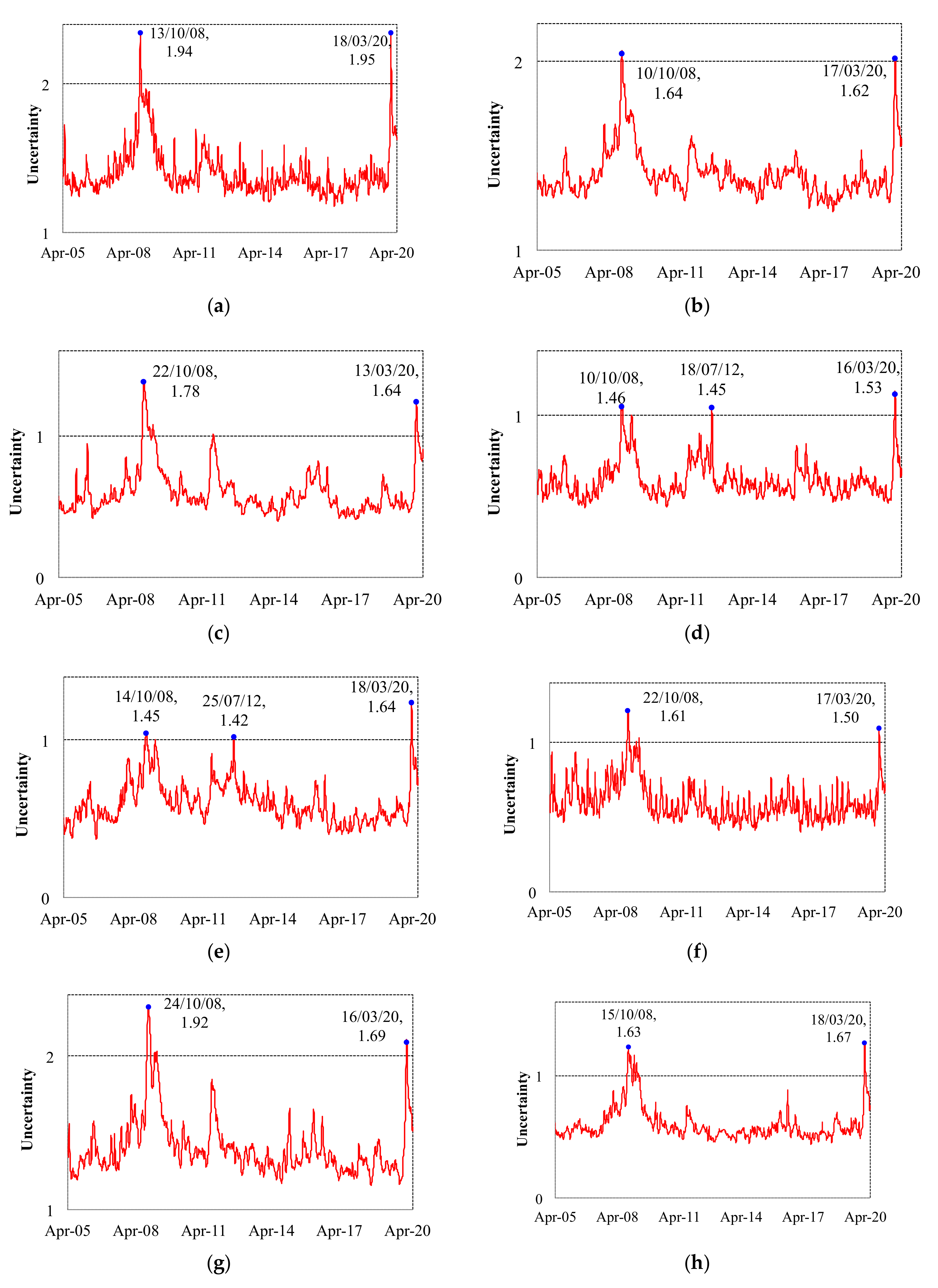
In
Figure 1a–h, we present the eight uncertainty indicators estimated for the European countries in our sample: Belgium, France, Germany, Italy, Spain, Sweden, Switzerland, and the United Kingdom, from 1 April 2005 to 25 June 2020 (see also the
Supplementary Materials). The indicators were normalized to have a mean equal to 1. A value of an indicator above 1 refers to a situation of relatively high uncertainty in a given day, while a value below 1 refers to a low-uncertainty period. Notice that the index being relative to each country’s own mean, eases the interpretation of the individual uncertainty dynamics in time, but it would be inaccurate to compare the level of uncertainty across countries.
The uncertainty indicator was constructed using daily data from stocks listed on the main national stock market index during the whole sample period spanning 1 April 2005–25 June 2020. An increment of the uncertainty indicator refers to an increase of generalized uncertainty in the market in a given day. The index was normalized to have a mean of one, thus, a value above one means that uncertainty was higher than the historical mean on that date, while a value below one means a relatively low aggregate uncertainty was recorded in the market.
As shown in
Figure 1a, the indicator reached a maximum, in Belgium, on 18 March 2020, when it equaled 1.95, which can be understood as a level of uncertainty 95% higher than the historical mean of the Brussels’ market, due to the coronavirus crisis.
All indicators recorded presented in
Figure 1 show high historical levels, between 1.5 and 2.0, during the recent coronavirus outbreak in the region, in middle March 2020, and before the massive liquidity interventions to the market carried out by the European Central Bank, the Bank of England, and the Federal Reserve. Nevertheless, while for some markets, such as Belgium, Italy, Spain and the United Kingdom, those levels correspond to a maximum within the sample period, for other countries such as France, Germany, Switzerland, and Sweden, although significantly larger than the average values, still the uncertainty levels in March 2020 were below the levels recorded in the wake of the Global Financial Crisis, in October 2008.
Figure 1b shows that the generalized uncertainty indicator reached a maximum, in France, on 10 October 2008, when it equaled 1.64, which can be understood as a level of uncertainty 64% higher than the historical mean of the market, due to the Global Financial Crisis. A level very similar to that reached on 17 March 2020 in the middle of the Covid-19 crisis: 1.62.
Although aggregate uncertainty dynamics shares common features, trends, and cycles across markets, there are also noticeable differences. For instance, in Spain, the difference between the uncertainty level during the Global Financial Crisis (GFC) (1.45) and the recent crisis due to the coronavirus (1.64), equals 19 basis points (bp), while the same difference is narrower for Italy (7 bp) and the United Kingdom (4 bp) or Belgium (1 bp). This means that, in relative terms, Spain was the market hit the most, in terms of uncertainty, in Europe.
The indicator reached a maximum, in Germany, 22 October 2008, when it equaled 1.78, which can be understood as a level of uncertainty 78% higher than the historical mean of the market, due to the Global Financial Crisis.
On the other hand, regarding the markets less affected by the recent lockdowns and other measures engaged to contain the outbreak of the virus, but more affected by the GFC in relatively terms, the differences in terms of uncertainty, from the largest to the smallest, were recorded in: Switzerland (23 bp), Germany (18 bp), Sweden (11 bp), and France (2 bp). That is, for markets such as Belgium or France, the impact of the two crises, independently of the different fundamentals and mechanisms underlying the two, was virtually the same.
The indicator reached a maximum, in Italy, on 16 March 2020, when it equaled 1.53, which can be understood as a level of uncertainty 53% higher than the historical mean of Milan’s market, due to the coronavirus crisis.
For some markets, the increments in uncertainty in the wake of the European debt crisis, particularly worrying for countries belonging to the European periphery, are well recorded by the proposed uncertainty indexes. This is the case most notably of Spain and Italy, but the increment in uncertainty was also notorious for Switzerland and Germany.
The indicator reached a maximum, in Spain, on 18 March 2020, when it equaled 1.64, which can be understood as a level of uncertainty 64% higher than the historical mean of such market, due to the coronavirus crisis. In the case of Sweden, on 24 October 2008, the maximum equaled 1.92 (i.e., a level of uncertainty 92% higher than the historical mean of the Stockholm’s market). The stock market in Switzerland witnessed a maximum on 22 October 2008, at 1.61, while the United Kingdom uncertainty peaked on 18 March 2020, when it equaled 1.67.
In
Table 1, we present some descriptive statistics of the uncertainty indicators, which help us to analyze uncertainty in different European markets. We report the standard deviation, skewness, kurtosis, persistence, and half-life of a shock in days. The persistence (
) is estimated using an autoregressive model of order one, and it corresponds to the coefficient of the first lag in the regression of the indicator of a given country on its past values. The half-life corresponds to the number of days that will take the market to absorb half of the impact of an uncertainty shock, and it is estimated using the formula
. The results show that Sweden will absorb the shock faster than other markets (116 days), while Germany will take longer (941 days). Germany and France have large markets with fewer small peaks, and therefore, it takes longer for those markets than for others to integrate shocks when they occur.
Table 2 shows the first two factors (except for Switzerland, which only has one factor). We construct the factors as linear combinations of the input returns, so our factors can be interpreted as financial portfolios. For this reason, they present the characteristics of financial time series, namely, leptokurtosis, negative skewness (most of the times), and mean close to zero.
5. Conclusions
This paper fills a gap in the literature of uncertainty indices by introducing the possibility to provide high-frequency indicators. In our case, we have presented the methodology to produce a daily uncertainty index from market data. Our contribution has a practical perspective, as it shows that daily uncertainty indices of stock market data were able to react quickly to the first outbursts of the corona crisis. These results have enormous implications for economic analysis and to assess the influence of policy interventions, which should be transmitted to the market in an expedited fashion. They also allow comparisons between regions and countries and to better understand how crises are transmitted or how markets may suffer from contagion.
We propose a methodology to estimate aggregate uncertainty using stock market information, which allows us to provide uncertainty measurements on a real-time basis. We estimate uncertainty for eight European markets, namely Belgium, France, Germany, Italy, Spain, Sweden, Switzerland, and the United Kingdom, from 1 April 2005 to 25 June 2020. We document similitudes in aggregate uncertainty dynamics in all the markets, which peak both during the Global Financial Crisis in 2008, and in the wake of the coronavirus pandemic in the middle of March 2020.
Our indicators put into perspective the market reaction of the last virus outbreak, which is not to be understood as triggering unprecedented levels of uncertainty for all the markets across Europe. Indeed, only for Spain, the maximum reached during the pandemic was significantly higher than the peaks recorded during the Global Financial Crisis or the European Debt Crisis in 2012. Finally, uncertainty is a very persistent phenomenon. We should expect to pass at least between half of a year and two and a half years for most of the impact of an uncertainty shock to be absorbed by the market.
One limitation of our methodology is that the index is based on the average levels, which means that this level changes each time new data are acquired. We believe that there could be other ways to stabilize the central tendency, so that the uncertainty index is not relative to the observed mean level, but we leave this point for future research.


