On the Construction of Some Deterministic and Stochastic Non-Local SIR Models

Abstract

Fractional-order epidemic models have become widely studied in the literature. Here, we consider the generalization of a simple $SIR$ model in the context of generalized fractional calculus and we study the main features of such model. Moreover, we construct semi-Markov stochastic epidemic models by using time changed continuous time Markov chains, where the parent process is the stochastic analog of a simple $SIR$ epidemic. In particular, we show that, differently from what happens in the classic case, the deterministic model does not coincide with the large population limit of the stochastic one. This loss of fluid limit is then stressed in terms of numerical examples.

1. Introduction

Starting from the seminal paper by Kermack and McKendrick [1], epidemic models have been a fruitful field of applications of dynamical systems. However, stochastic models for epidemic were already proposed by McKendrick in [2]. Starting from these papers, different epidemic models, both deterministic and stochastic, have been considered. The approach we focus on in this paper is the Continuous-Time Markov Chain one, used for instance by [3] and then successively extended to different deterministic models (see, e.g., [4,5] and references therein). For more recent works, we refer, for instance, to those of Ball [6] (in which the authors describe some exact results on the distribution of final size of the epidemics), Lefѐvre and Simon [7] (for a matrix analysis approach), Ball et al. [8] (in which social distancing is modeled in terms of adaptive random graphs), and Liu et al. [9] (in which the authors modeled environmental noise via Lévy jumps).

In modern times, epidemic models with information variables have been considered, in the context of behavioral epidemiology (to cite a contemporary paper, see [10], which deals with the COVID-19 pandemic). The information variable in behavioral epidemiology is a first important example of the introduction of memory effects in deterministic epidemic models (see, e.g., [11,12,13]). Indeed, the information variable can be modeled as the convolution product between a function of the state of the system (representing the information that individuals consider relevant) and a memory kernel (representing the weight that individuals give to the past history of the system).

In stochastic epidemic modeling, instead, the necessity of introducing some memory effects is solved by considering semi-Markov epidemic models (in place of Markov ones), which, however, are more difficult to handle (see, e.g., [14]).

With the idea of introducing memory effects in mind, we can consider the case of non-integer order epidemic models. Indeed, fractional calculus operators (e.g., the Caputo fractional derivative) are non-local convolution operators that weight in some sense the variation of a function during its entire lifetime. To cite some fractional-order epidemic models, let us recall the works of Diethelm [15] concerning outbreaks of dengue fever and dos Santos et al. [16] for some bovine diseases, as well as simpler models (e.g., [17,18]). All these models are strictly linked with the introduction of fractional-order dynamical systems, as in [19,20]. Let us also recall that fractional-order models could also arise as one consider continuous-time random walk approaches to construct epidemic models (see, e.g., [21]). The advantage of taking in consideration fractional-order models (or non-local models in general) is the fact that the modeled dynamics does not depend on the instantaneous state of the system, but on the whole history of it. In a certain sense, as the information variable is introduced to model human behavior depending on the information individuals have on the history of the epidemic, non-local models take in consideration memory effects on the epidemic that do not depend on human behavior but on the characteristic of the epidemic itself.

Concerning population models, one obtains analogous fractional-order stochastic models (or more general non-local models) by using time-changed continuous-time Markov chains, as one can see, for instance, in [22,23,24,25]. This fractionalization procedure leads to non-local stochastic models which are in some sense the counterpart of non-local deterministic ones. However, this procedure works due to the linear nature of the considered models. Even the simpler $SIR$ model with linear force of infection admits a non-linearity, hence we cannot expect that non-local $SIR$ models (obtained by a naive substitution of the time-derivative with a non-local operator) correspond directly to time-changed stochastic $SIR$ models.

This paper focuses on introducing some general non-local $SIR$ model by such kind of naive substitution in terms of Caputo-type non-local derivative induced by Bernstein functions (see [26,27,28]) and then some time-changed (by means of inverse subordinators) stochastic $SIR$ models. Concerning the deterministic case, we aim to introduce some alternative models with respect to the fractional-order ones, to work with different memory kernels. On the other hand, time-changed models constitute an interesting class of semi-Markov stochastic models, which, as stated above, are more natural to consider.

After a preliminary introduction of the main tools, given in Section 2, in Section 3, we give a qualitative study of the non-local $SIR$ model, illustrating the main differences with respect to the classical one. After that, we first recall some main properties of the stochastic $SIR$ model in Section 4 and then in Section 5 we consider its time-changed version. In particular, we show that the state probabilities of the process solve a system of non-local difference-differential equations and their expected values solve a system of two non-local differential equations that resembles in some sense the non-local $SIR$ model introduced in Section 3 (despite not being equal, due to the non-linearity of the $SIR$ model). We also show that a side effect of the time-change is a delay in the epidemic dynamics. In Section 6, we study large population limits of the time-changed $SIR$ model. The result we obtain is a sort of negative result: the usual fluid limit of the stochastic $SIR$ model is not preserved by the time-change, and then the non-local $SIR$ model cannot be seen as a mean field behavior of the time-changed model. In Section 7, we show some numerical evidence supporting our negative results. Conclusive observations are then considered in Section 8.

However, let us anticipate an important feature one has to take in consideration when working with non-local $SIR$ models (both deterministic and stochastic). Such kind of models do not adapt well to epidemics for which the number of infective is approximatively diffusive or super-diffusive in time (i.e., if the number of infective exhibits a variance of the form $C{t}^{\gamma }$ with $\gamma \ge 1$, see, e.g., [29]), thus limiting the field of applications. In particular, there is evidence that the Coronavirus infectious disease 2019 (COVID-2019) admits a super-diffusive behavior in some contexts (see, e.g., [30,31]), hence these models should not be applied to describe such infectious disease in the super-spreading environment.

2. Inverse Subordinators and Non-Local Convolution Derivatives

Before introducing the actual model, let us give some preliminaries on the non-local operators we use in the following. Let us fix in the whole text a filtered probability space $(\mathsf{\Omega },\mathcal{F},{\mathcal{F}}_t,\mathbb{P})$.

Definition 1.

We say that $\mathsf{\Phi }:[0,+\infty )\to \mathbb{R}$ is aBernstein functionif $\mathsf{\Phi }\in C^{\infty }\left({\mathbb{R}}^{+}\right)$ (where we denote ${\mathbb{R}}^{+}=(0,+\infty )$), $\mathsf{\Phi }\left(\lambda \right)\ge 0$ for any $\lambda \ge 0$ and, for any $n\in \mathbb{N}$ and $\lambda \ge 0$,

$${(-1)}^n\frac{d^n\mathsf{\Phi }}{d{\lambda }^n}\left(\lambda \right)\le 0.$$

For generalities on Bernstein functions, we refer to [32]. Let us denote by $\mathcal{BF}$ the convex cone of Bernstein functions. For any $\mathsf{\Phi }\in \mathcal{BF}$, there exists a unique triplet $(a_{\mathsf{\Phi }},b_{\mathsf{\Phi }},{\nu }_{\mathsf{\Phi }})$, where $a_{\mathsf{\Phi }},b_{\mathsf{\Phi }}\ge 0$ and ${\nu }_{\mathsf{\Phi }}\left(dt\right)$ is a measure on $(0,+\infty )$ with the integrability property

$${\int }_0^{+\infty }(1\wedge t){\nu }_{\mathsf{\Phi }}\left(dt\right)<+\infty ,$$

such that

$$\mathsf{\Phi }\left(\lambda \right)=a_{\mathsf{\Phi }}+b_{\mathsf{\Phi }}\lambda +{\int }_0^{+\infty }(1-e^{-\lambda t}){\nu }_{\mathsf{\Phi }}\left(dt\right).$$

(1)

The triple $(a_{\mathsf{\Phi }},b_{\mathsf{\Phi }},{\nu }_{\mathsf{\Phi }})$ is said to be the characteristic triple of $\mathsf{\Phi }$ and ${\nu }_{\mathsf{\Phi }}$ is the Lévy measure of $\mathsf{\Phi }$.

Moreover, let us recall that for each Bernstein function $\mathsf{\Phi }\in \mathcal{BF}$ there exists a subordinator ${\sigma }_{\mathsf{\Phi }}\left(t\right)$ (i.e., an increasing Lévy process) such that

$$\mathbb{E}\left[e^{-\lambda {\sigma }_{\mathsf{\Phi }}\left(y\right)}\right]=e^{-y\mathsf{\Phi }\left(\lambda \right)},y\ge 0,\lambda \ge 0.$$

In the following, we always consider $a_{\mathsf{\Phi }}=b_{\mathsf{\Phi }}=0$ and ${\nu }_{\mathsf{\Phi }}(0,+\infty )=+\infty$. As $a_{\mathsf{\Phi }}=0$, we know that the subordinator ${\sigma }_{\mathsf{\Phi }}$ is not killed. Moreover, since $b_{\mathsf{\Phi }}=0$ and ${\nu }_{\mathsf{\Phi }}(0,+\infty )=+\infty$, we know that ${\sigma }_{\mathsf{\Phi }}$ is a pure jump strictly increasing process (see [33]).

Definition 2.

Given a subordinator ${\sigma }_{\mathsf{\Phi }}\left(t\right)$, we define the inverse subordinator associated to Φ as the process

$$L_{\mathsf{\Phi }}\left(t\right)=inf\{y\ge 0:{\sigma }_{\mathsf{\Phi }}\left(y\right)>t\}.$$

From now on, let us denote ${\overline{\nu }}_{\mathsf{\Phi }}\left(t\right)={\nu }_{\mathsf{\Phi }}(t,+\infty )$ and $g_{\mathsf{\Phi }}(ds;y)$ the law of the random variable ${\sigma }_{\mathsf{\Phi }}\left(y\right)$. In [34], it is shown that $L_{\mathsf{\Phi }}\left(t\right)$ admits a probability density function $f_{\mathsf{\Phi }}(s;t)$ given by

$$f_{\mathsf{\Phi }}(s;t)={\int }_0^{+\infty }{\overline{\nu }}_{\mathsf{\Phi }}(t-\tau )g_{\mathsf{\Phi }}(d\tau ;s).$$

Moreover, denoting by ${\mathcal{L}}_{t\to \lambda }$ the Laplace transform operator, it holds that

$${\mathcal{L}}_{t\to \lambda }\left[f_{\mathsf{\Phi }}(s;t)\right]\left(\lambda \right)=\frac{\mathsf{\Phi }\left(\lambda \right)}{\lambda }{e}^{-s\mathsf{\Phi }\left(\lambda \right)},$$

and

$${\mathcal{L}}_{t\to \lambda }\left[{\overline{\nu }}_{\mathsf{\Phi }}\left(t\right)\right]\left(\lambda \right)=\frac{\mathsf{\Phi }\left(\lambda \right)}{\lambda },$$

(2)

for any $\lambda >0$. Now, we can introduce the non-local convolution derivatives (of Caputo type) associated with $\mathsf{\Phi }$, as given in [26,27].

Definition 3.

Let $u:{\mathbb{R}}^{+}\to \mathbb{R}$ be an absolutely continuous function. Then, we define the non-local convolution derivative induced by Φ of u as

$$\frac{d^{\mathsf{\Phi }}u}{d{t}^{\mathsf{\Phi }}}\left(t\right)={\int }_0^t{u}^{\prime }\left(\tau \right){\overline{\nu }}_{\mathsf{\Phi }}(t-\tau )d\tau .$$

(3)

Remark 1.

In analogy of what is usually done with Riemann–Liouville and Caputo derivatives, one can introduce the following regularized non-local derivative

$$\frac{d^{\mathsf{\Phi }}u}{d{t}^{\mathsf{\Phi }}}\left(t\right)=\frac{d}{dt}{\int }_0^t(u\left(\tau \right)-u(0+))\overline{\nu }(t-\tau )d\tau$$

(4)

observing that it coincides with the previous definition on absolutely continuous functions.

Remark 2.

Let us observe that, if $\mathsf{\Phi }\left(\lambda \right)={\lambda }^{\alpha }$, for $\alpha \in (0,1)$, the operator $\frac{d^{\mathsf{\Phi }}}{d{t}^{\mathsf{\Phi }}}$ coincides with the usual fractional Caputo derivative.

Let us recall that, if both u and $\frac{d^{\mathsf{\Phi }}u}{d{t}^{\mathsf{\Phi }}}$ are Laplace transformable, then

$${\mathcal{L}}_{t\to \lambda }\left[\frac{d^{\mathsf{\Phi }}u}{d{t}^{\mathsf{\Phi }}}\left(t\right)\right]\left(\lambda \right)=\mathsf{\Phi }\left(\lambda \right){\mathcal{L}}_{t\to \lambda }\left[u\left(t\right)\right]\left(\lambda \right)+\frac{\mathsf{\Phi }\left(\lambda \right)}{\lambda }u\left(0^{+}\right).$$

We are interested in the eigenfunctions of such operators. It can be shown, by Laplace transform arguments (see, e.g., [28,35]) or Green functions arguments (see [36]), that the (eigenvalue) Cauchy problem

$$\left\{\begin{array}{cc}{\displaystyle \frac{d^{\mathsf{\Phi }}{\mathfrak{e}}_{\mathsf{\Phi }}}{d{t}^{\mathsf{\Phi }}}(t;\lambda )=\lambda {\mathfrak{e}}_{\mathsf{\Phi }}(t;\lambda )}\hfill & t>0\hfill \\ {\mathfrak{e}}_{\mathsf{\Phi }}(0;\lambda )=1\hfill \end{array}\right.$$

admits a unique solution for any $\lambda \in \mathbb{R}$ and it is given by ${\mathfrak{e}}_{\mathsf{\Phi }}(t;\lambda ):=\mathbb{E}\left[e^{\lambda E_{\mathsf{\Phi }}\left(t\right)}\right]$ (hence, in particular, it is a completely monotone function in the variable $-\lambda \in [0,+\infty )$ for fixed t).

Remark 3.

Let us recall that, if $\mathsf{\Phi }\left(\lambda \right)={\lambda }^{\alpha }$, then ${\mathfrak{e}}_{\mathsf{\Phi }}(t;\lambda )=E_{\alpha }\left(\lambda t^{\alpha }\right)$ where

$$E_{\alpha }\left(t\right):=\sum _{k=0}^{+\infty }\frac{t^k}{\mathsf{\Gamma }(\alpha k+1)},t\ge 0$$

is the one-parameter Mittag–Leffler function (see [37]).

We are also interested in the following subclass of Bernstein functions.

Definition 4.

Let $\mathsf{\Phi }\in \mathcal{BF}$. We say that Φ is a special Bernstein function if ${\mathsf{\Phi }}^{★}\left(\lambda \right)=\frac{\lambda }{\mathsf{\Phi }\left(\lambda \right)}$ is still a Bernstein function, called the conjugate Bernstein function.

Let us denote by $\mathcal{SBF}$ the class of special Bernstein functions. If $\mathsf{\Phi }\in \mathcal{SBF}$, we call ${\sigma }_{\mathsf{\Phi }}$ a special subordinator. Let us also introduce the renewal function of ${\sigma }_{\mathsf{\Phi }}$

$$U_{\mathsf{\Phi }}\left(t\right)=\mathbb{E}\left[L_{\mathsf{\Phi }}\left(t\right)\right],t\ge 0.$$

Under the assumption $a_{\mathsf{\Phi }}=b_{\mathsf{\Phi }}=0$ and ${\nu }_{\mathsf{\Phi }}(0,+\infty )=+\infty$, if $\mathsf{\Phi }\in \mathcal{SBF}$, we know there exists a non-increasing non-negative function $u_{\mathsf{\Phi }}\left(t\right)$ such that

$$U_{\mathsf{\Phi }}\left(dt\right)=u_{\mathsf{\Phi }}\left(t\right)dt,$$

called the potential density of ${\sigma }_{\mathsf{\Phi }}$.

In [38], it is shown that, for any absolutely continuous function $f\left(t\right)$, it holds that

$${\mathcal{I}}_t^{\mathsf{\Phi }}\frac{d^{\mathsf{\Phi }}f}{d{t}^{\mathsf{\Phi }}}\left(t\right)=f\left(0\right)+f\left(t\right),$$

where ${\mathcal{I}}_t^{\mathsf{\Phi }}$ is defined as

$${\mathcal{I}}_t^{\mathsf{\Phi }}g\left(t\right)={\int }_0^t{u}_{\mathsf{\Phi }}(t-\tau )g\left(\tau \right)d\tau .$$

In particular, if g is Laplace transformable, it holds that

$${\mathcal{L}}_{t\to \lambda }\left[{\mathcal{I}}_t^{\mathsf{\Phi }}g\left(t\right)\right]\left(\lambda \right)=\frac{1}{\mathsf{\Phi }\left(\lambda \right)}{\mathcal{L}}_{t\to \lambda }\left[g\left(t\right)\right]\left(\lambda \right).$$

By using such property, we can show the following comparison principle.

Proposition 1.

Let $\mathsf{\Phi }\in \mathcal{SBF}$. Suppose $x\left(t\right),y\left(t\right)$ are Laplace transformable with their non-local convolution derivatives and such that $x\left(0\right)\le y\left(0\right)$ and $\frac{d^{\mathsf{\Phi }}x}{d{t}^{\mathsf{\Phi }}}\left(t\right)\le \frac{d^{\mathsf{\Phi }}y}{d{t}^{\mathsf{\Phi }}}\left(t\right)$ for any $t\ge 0$. Then, $x\left(t\right)\le y\left(t\right)$ for any $t\ge 0$.

Proof. 

Let us consider $\frac{d^{\mathsf{\Phi }}}{d{t}^{\mathsf{\Phi }}}y\left(t\right)=\xi \left(t\right)+\frac{d^{\mathsf{\Phi }}}{d{t}^{\mathsf{\Phi }}}x\left(t\right)$ for some function $\xi \left(t\right)\ge 0$ that is Laplace transformable by hypotheses. Let us take the Laplace transform on both sides to obtain

$$\mathsf{\Phi }\left(\lambda \right)\mathcal{L}\left[y\right]\left(\lambda \right)-\frac{\mathsf{\Phi }\left(\lambda \right)}{\lambda }y\left(0\right)=\mathcal{L}\left[\xi \right]\left(\lambda \right)+\mathsf{\Phi }\left(\lambda \right)\mathcal{L}\left[x\right]\left(\lambda \right)-\frac{\mathsf{\Phi }\left(\lambda \right)}{\lambda }x\left(0\right).$$

Dividing everything by $\mathsf{\Phi }\left(\lambda \right)$, we have

$$\mathcal{L}\left[y\right]\left(\lambda \right)-\mathcal{L}\left[x\right]\left(\lambda \right)=\frac{1}{\mathsf{\Phi }\left(\lambda \right)}\mathcal{L}\left[\xi \right]\left(\lambda \right)+\frac{1}{\lambda }(x\left(0\right)-y\left(0\right)).$$

Now, let us take the inverse Laplace transform to obtain

$$y\left(t\right)-x\left(t\right)={\mathcal{I}}^{\mathsf{\Phi }}\xi \left(t\right)+(y\left(0\right)-x\left(0\right))\ge 0,$$

concluding the proof. □

From now on, let us consider $\mathsf{\Phi }\in \mathcal{SBF}$. We can also show a generalized mean value theorem, following the lines of ([39] Theorem 1).

Theorem 1.

Let $f,\frac{d^{\mathsf{\Phi }}f}{d{t}^{\mathsf{\Phi }}}$ be continuous in $[0,T]$ and consider $t\in (0,T]$. Then, there exists $\xi \in (0,t)$ such that

$$f\left(t\right)=f\left(0\right)+\frac{d^{\mathsf{\Phi }}f}{d{t}^{\mathsf{\Phi }}}\left(\xi \right)U_{\mathsf{\Phi }}\left(t\right).$$

(5)

Proof. 

Let us observe that, by definition,

$${\mathcal{I}}_t^{\mathsf{\Phi }}\frac{d^{\mathsf{\Phi }}f}{d{t}^{\mathsf{\Phi }}}\left(t\right)={\int }_0^t{u}_{\mathsf{\Phi }}(t-\tau )\frac{d^{\mathsf{\Phi }}f}{d{t}^{\mathsf{\Phi }}}\left(\tau \right)d\tau .$$

By the integral mean value theorem, we know that there exists $\xi \in (0,t)$ such that

$${\mathcal{I}}_t^{\mathsf{\Phi }}\frac{d^{\mathsf{\Phi }}f}{d{t}^{\mathsf{\Phi }}}\left(t\right)=\frac{d^{\mathsf{\Phi }}f}{d{t}^{\mathsf{\Phi }}}\left(\xi \right){\int }_0^t{u}_{\mathsf{\Phi }}(t-\tau )d\tau =\frac{d^{\mathsf{\Phi }}f}{d{t}^{\mathsf{\Phi }}}\left(\xi \right)U_{\mathsf{\Phi }}\left(t\right).$$

On the other hand, we have

$${\mathcal{I}}_t^{\mathsf{\Phi }}\frac{d^{\mathsf{\Phi }}f}{d{t}^{\mathsf{\Phi }}}\left(t\right)=f\left(t\right)-f\left(0\right)$$

thus Equation (5) holds. □

Let us finally recall the following definition, which is useful in what follows.

Definition 5.

A function $f:[0,+\infty )\to \mathbb{R}$ is said to be regularly varying at ∞ of order $\alpha \in \mathbb{R}$ if for any $c>0$

$$\underset{t\to +\infty }{lim}\frac{f\left(ct\right)}{f\left(t\right)}=c^{\alpha }.$$

We say that f isregularly varyingat $0^{+}$ of order $\alpha \in \mathbb{R}$ if $f(1/t)$ is regularly varying at infinity of order α.

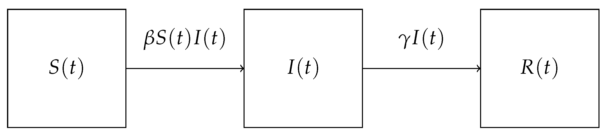
3. A Non-Local SIR Model

Let us consider the following model

$$\left\{\begin{array}{c}{\displaystyle \frac{d^{\mathsf{\Phi }}{S}^{\mathsf{\Phi }}\left(t\right)}{d{t}^{\mathsf{\Phi }}}=-\beta S^{\mathsf{\Phi }}\left(t\right)I^{\mathsf{\Phi }}\left(t\right)}\hfill \\ {\displaystyle \frac{d^{\mathsf{\Phi }}{I}^{\mathsf{\Phi }}\left(t\right)}{d{t}^{\mathsf{\Phi }}}=\beta S^{\mathsf{\Phi }}\left(t\right)I^{\mathsf{\Phi }}\left(t\right)-\gamma I^{\mathsf{\Phi }}\left(t\right)}\hfill \\ {\displaystyle \frac{d^{\mathsf{\Phi }}{R}^{\mathsf{\Phi }}\left(t\right)}{d{t}^{\mathsf{\Phi }}}=\gamma I^{\mathsf{\Phi }}\left(t\right),}\hfill \end{array}\right.$$

(6)

where $\beta ,\gamma >0$ are, respectively, the infection parameter and the removal parameter. A schematization of the compartments of the model is given in Figure 1.

Figure 1. Schematization of the $SIR$ model with linear force of infection and without population dynamics.

This model constitute a non-local counterpart to the simple $SIR$ model without population dynamics. By existence and uniqueness of uniformly bounded solutions (see [28]), we have that $S^{\mathsf{\Phi }}\left(t\right)+I^{\mathsf{\Phi }}\left(t\right)+R^{\mathsf{\Phi }}\left(t\right)=N$, where N is a fixed constant. Let us set for simplicity $N=1$. In such way, we can consider $S^{\mathsf{\Phi }}\left(t\right)$, $I^{\mathsf{\Phi }}\left(t\right)$, and $R^{\mathsf{\Phi }}\left(t\right)$ to be, respectively, the density of susceptible, infected, and removed entities in the population. In particular, we can recover $R^{\mathsf{\Phi }}\left(t\right)=1-S^{\mathsf{\Phi }}\left(t\right)-I^{\mathsf{\Phi }}\left(t\right)$, thus we only need to study the dynamics of $S^{\mathsf{\Phi }}\left(t\right)$ and $I^{\mathsf{\Phi }}\left(t\right)$, through the system

$$\left\{\begin{array}{c}{\displaystyle \frac{d^{\mathsf{\Phi }}{S}^{\mathsf{\Phi }}\left(t\right)}{d{t}^{\mathsf{\Phi }}}=-\beta S^{\mathsf{\Phi }}\left(t\right)I^{\mathsf{\Phi }}\left(t\right)}\hfill \\ {\displaystyle \frac{d^{\mathsf{\Phi }}{I}^{\mathsf{\Phi }}\left(t\right)}{d{t}^{\mathsf{\Phi }}}=\beta S^{\mathsf{\Phi }}\left(t\right)I^{\mathsf{\Phi }}\left(t\right)-\gamma I^{\mathsf{\Phi }}\left(t\right).}\hfill \end{array}\right.$$

(7)

As a first step, we need to show that both $S^{\mathsf{\Phi }}\left(t\right)$ and $I^{\mathsf{\Phi }}\left(t\right)$ are non-negative if we start from initial datum $S_0,I_0>0$. To do this, let us first observe that, by existence and uniqueness of uniformly bounded solutions (see [28] Corollary 4.6 for the linear case: the proof can be easily adapted to the bilinear case), we have that the equilibrium points of the dynamical system are of the form $(S_{*},0)$. Indeed, if $(S\left(0\right),I\left(0\right))=(S_{*},0)$, then the unique solution of the system is given by $(S^{\mathsf{\Phi }}\left(t\right),I^{\mathsf{\Phi }}\left(t\right))\equiv (S_{*},0)$. Now, we can show the following proposition.

Proposition 2.

Let $(S^{\mathsf{\Phi }}\left(t\right),I^{\mathsf{\Phi }}\left(t\right))$ be a solution of Equation (7) such that

$$(S^{\mathsf{\Phi }}\left(0\right),I^{\mathsf{\Phi }}\left(0\right))=(S_0,I_0)$$

with $S_0,I_0>0$. Then, $S^{\mathsf{\Phi }}\left(t\right),I^{\mathsf{\Phi }}\left(t\right)>0$.

Proof. 

Let us first observe that $(S^{\mathsf{\Phi }}\left(t\right),I^{\mathsf{\Phi }}\left(t\right))$ cannot leave the ${\mathbb{R}}_{+}^2$ quadrant (where ${\mathbb{R}}_{+}^2=\{(x,y)\in {\mathbb{R}}^2:x>0,y>0\}$) through a point of the form $(S_{*},0)$ for $S_{*}\ge 0$ by existence and uniqueness of uniformly bounded solutions. To show that if we start from $(S_0,I_0)\in {\mathbb{R}}_{+}^2$ we cannot leave the ${\mathbb{R}}_{+}^2$ quadrant through a point $(0,I_{*})$ with $I_{*}>0$, let us show that for any $I_{*}>0$ we can construct a solution $(S^{\mathsf{\Phi }}\left(t\right),I^{\mathsf{\Phi }}\left(t\right))$ starting from a certain $(0,I_0)$ with $I_0>0$ and such that $S^{\mathsf{\Phi }}\left(t\right)\equiv 0$ and $I\left(t_{*}\right)=I_{*}$ for any fixed $t_{*}>0$.

To do this, let us observe that, if we consider $S\left(0\right)=0$ and $I\left(0\right)=I_0$, then we have $S^{\mathsf{\Phi }}\left(t\right)\equiv 0$ and

$$I^{\mathsf{\Phi }}\left(t\right)=I_0{\mathfrak{e}}_{\mathsf{\Phi }}(t,-\gamma ).$$

Let us fix $I_{*}>0$ and $t_{*}>0$. Then, choosing

$$I_0=\frac{I_{*}}{{\mathfrak{e}}_{\mathsf{\Phi }}(t_{*},-\gamma )}$$

we have found a solution $(S^{\mathsf{\Phi }}\left(t\right),I^{\mathsf{\Phi }}\left(t\right))$ such that $(S\left(t_{*}\right),I\left(t_{*}\right))=(0,I_{*})$. Thus, by existence and uniqueness of uniformly bounded solutions, $(S^{\mathsf{\Phi }}\left(t\right),I^{\mathsf{\Phi }}\left(t\right))$ cannot leave the ${\mathbb{R}}_{+}^2$ quadrant through $(0,I_{*})$. □

As a corollary, we also obtain that $I^{\mathsf{\Phi }}\left(t\right)+S^{\mathsf{\Phi }}\left(t\right)\le 1$.

Corollary 1.

Let $(S^{\mathsf{\Phi }}\left(t\right),I^{\mathsf{\Phi }}\left(t\right))$ be a solution of Equation (7) such that

$$(S^{\mathsf{\Phi }}\left(0\right),I^{\mathsf{\Phi }}\left(0\right))=(S_0,I_0)$$

with $S_0,I_0>0$ and $S_0+I_0=1$. Then, $0<S^{\mathsf{\Phi }}\left(t\right)+I^{\mathsf{\Phi }}\left(t\right)\le 1$.

Proof. 

By the previous proposition, we know that $I^{\mathsf{\Phi }}\left(t\right)>0$ for any $t>0$. Moreover, since $S_0+I_0=1$, we have that $R\left(0\right)=R_0=0$. By the comparison principle in Proposition 1, we know that $R^{\mathsf{\Phi }}\left(t\right)\ge 0$ for any $t>0$. We conclude the proof observing that this implies $S^{\mathsf{\Phi }}\left(t\right)+I^{\mathsf{\Phi }}\left(t\right)\le 1$. □

As stated above, the equilibrium points are given by $(S_{*},0)$ where $S_{*}\in [0,1]$. Moreover, since $S^{\mathsf{\Phi }}\left(t\right),I^{\mathsf{\Phi }}\left(t\right)>0$, we can use the generalized mean value theorem to conclude that if $S\left(0\right)=S_0\in (0,1)$, then $S^{\mathsf{\Phi }}\left(t\right)\le S_0$. In particular, this means that

$$\frac{d^{\mathsf{\Phi }}{I}^{\mathsf{\Phi }}\left(t\right)}{d{t}^{\mathsf{\Phi }}}\le (\beta S_0-\gamma )I^{\mathsf{\Phi }}\left(t\right).$$

The comparison principle implies that $I^{\mathsf{\Phi }}\left(t\right)\le I_0{\mathfrak{e}}_{\mathsf{\Phi }}(t,\beta S_0-\gamma )$. Thus, if $\beta S_0-\gamma <0$, we have that $I^{\mathsf{\Phi }}\left(t\right)\to 0$ as $t\to +\infty$.

If $\beta S_0-\gamma =0$, we still have $S^{\mathsf{\Phi }}\left(t\right)\le S_0$. Moreover, $I\left(0\right)=I_0$ implies that there exists a time $\epsilon$ such that $I^{\mathsf{\Phi }}\left(t\right)>\frac{I_0}{2}$ for any $t\in (0,\epsilon )$. Let us define the maps $\psi =({\psi }^1,{\psi }^2)$ and $\theta =({\theta }^1,{\theta }^2)$ as in Theorem A1. In particular, for $s\in (0,\epsilon )$,

$$\begin{array}{c}{\theta }^1(t,s,\psi (·,(S_0,I_0)))=S_0-\beta {\int }_0^s{u}_{\mathsf{\Phi }}(t+s-\tau )S\left(\tau \right)I\left(\tau \right)d\tau \hfill \\ \hfill \le S_0-\beta \frac{I_0}{2}{\int }_0^s{u}_{\mathsf{\Phi }}(t+s-\tau )S\left(\tau \right)d\tau <S_0.\end{array}$$

In particular, we have that

$$\underset{t\to +\infty }{lim}\psi (t+s,(S_0,I_0))=\underset{t\to +\infty }{lim}\psi (t,\theta (t,s,\psi (·,(S_0,I_0))))=0$$

since $\beta {\theta }^1(t,s,\psi (·,(S_0,I_0)))-\gamma <0$.

As in the ordinary case, we can define the basic reproductive number as ${\mathcal{R}}_0=\frac{\beta S_0}{\gamma }$. With the previous observations, we show the following result.

Proposition 3.

If ${\mathcal{R}}_0\le 1$, then $I^{\mathsf{\Phi }}\left(t\right)\le I_0$ for any $t\ge 0$ and ${lim}_{t\to +\infty }{I}^{\mathsf{\Phi }}\left(t\right)=0$.

Remark 4.

In the case ${\mathcal{R}}_0>1$, we have that, at least for short times, by the comparison principle, $I^{\mathsf{\Phi }}\left(t\right)\ge I_0$. However, we could conclude that even in this case ${lim}_{t\to +\infty }{I}^{\mathsf{\Phi }}\left(t\right)=0$ if we are able to show that there exists a time $s>0$ for which ${\theta }^1(t,s,\psi (·,(S_0,I_0)))<\frac{\gamma }{\beta }$. This new condition (with respect to the ordinary case) is due to the lack of semigroup property of the flow $\psi (·,(S_0,I_0))$, together with the fact that we do not have any asymptote theorem for non-local derivatives. However, numerical examples, at least in the fractional-order case, seem to confirm the fact that ${lim}_{t\to +\infty }{I}^{\mathsf{\Phi }}\left(t\right)=0$ even if ${\mathcal{R}}_0>1$.

4. Some Generalities on the Stochastic SIR Model

Let us now give some generalities on the (simple) stochastic SIR model. We prevalently follow the lines of Daley and Gani [4]. First, let us construct a SIR model by denoting with $S^1\left(t\right)$ the number of susceptible individuals, $I^1\left(t\right)$ the number of infective individuals, and $R^1\left(t\right)$ the number of removed individuals at time $t>0$. Suppose the population is closed, that is to say there exists a constant $N\in \mathbb{N}$ such that

$$S^1\left(t\right)+I^1\left(t\right)+R^1\left(t\right)=N$$

Thus, we can deduce $R^1\left(t\right)$ from $S^1\left(t\right)$ and $I^1\left(t\right)$ simply imposing $R^1\left(t\right)=N-S^1\left(t\right)-I^1\left(t\right)$. Thus, we are interested in the bivariate process $(S^1\left(t\right),I^1\left(t\right))$, which is a Continuous Time Markov Chain. Let us consider as state space the set

$$\mathcal{S}=\{(s,i)\in {\mathbb{N}}_0^2:s+i\le N\}.$$

Now, let us define $\beta ,\gamma >0$ as the infection and removal parameters, respectively, as done in the previous section. Let us denote the transition probability functions as

$$p_1(t_2,(s_2,i_2);t_1,(s_1,i_1))=\mathbb{P}((S^1\left(t_2\right),I^1\left(t_2\right))=(s_2,i_2)|(S^1\left(t_1\right),I^1\left(t_1\right))=(s_1,i_1)).$$

Then, for any $(s,i)\in \mathcal{S}$ and $(s_2,i_2)\in \mathcal{S}\setminus \{(s,i),(s-1,i+1),(s,i-1)\}$, it holds that

$$\begin{array}{cc}\hfill p_1(t+\delta t,(s,i-1);t,(s,i))& =\gamma i\delta t+o\left(\delta t\right)\hfill \\ \hfill p_1(t+\delta t,(s-1,i+1);t,(s,i))& =\beta si\delta t+o\left(\delta t\right)\hfill \\ \hfill p_1(t+\delta t,(s,i);t,(s,i))& =1-i(\beta s-\gamma )\delta t+o\left(\delta t\right)\hfill \\ \hfill p_1(t+\delta t,(s_2,i_2);t,(s,i))& =o\left(\delta t\right).\hfill \end{array}$$

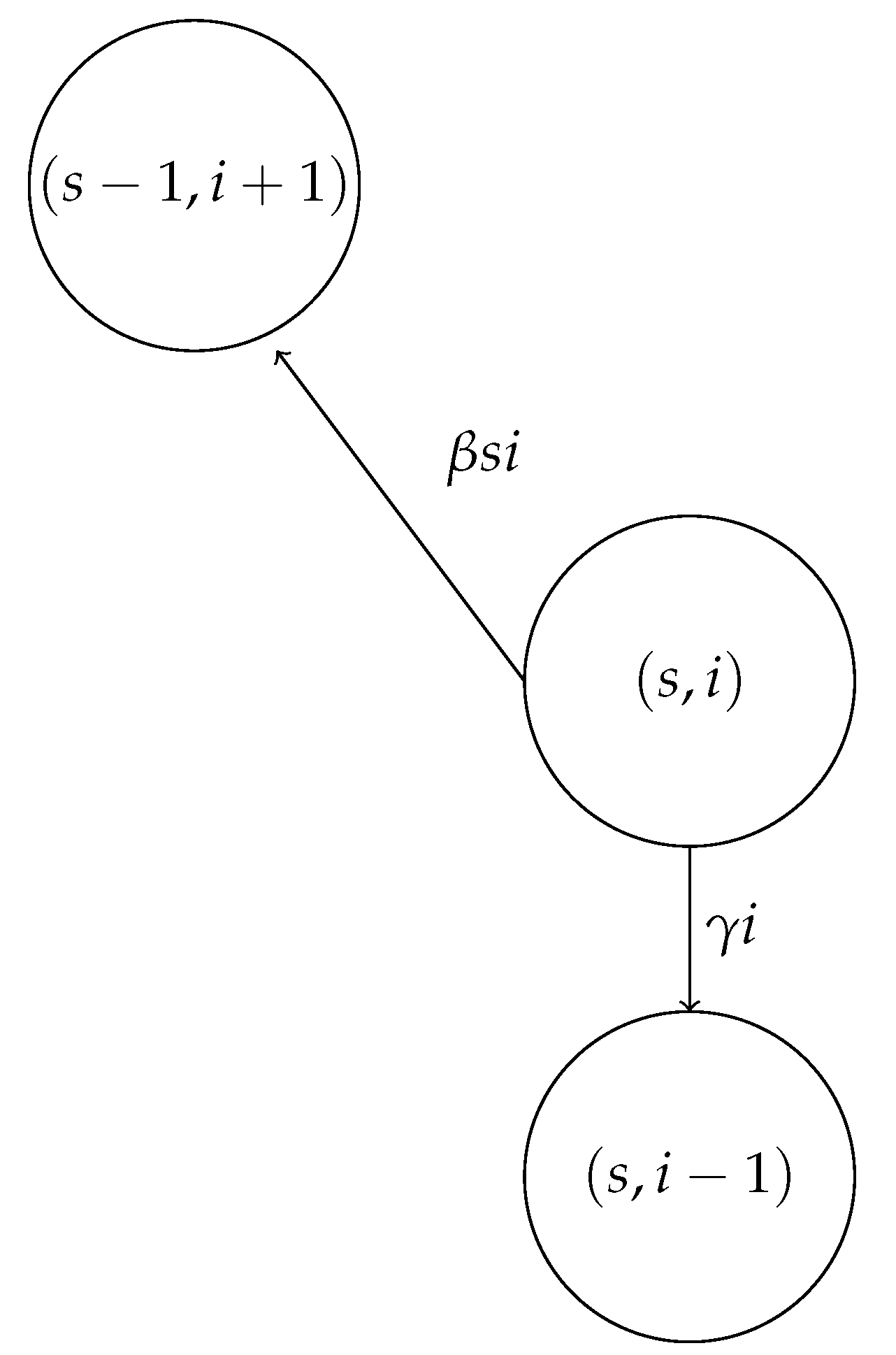
These transition probability functions are compatible with the choice of the state space, since it is easy to see that $S^1\left(t\right)+I^1\left(t\right)\le N$ and $S^1\left(t\right),I^1\left(t\right)\ge 0$ for any $t\ge 0$. A graphical schematization of the bivariate chain $(S_1\left(t\right),I_1\left(t\right))$ is given in Figure 2.

Figure 2. Schematization of a node for the stochastic $SIR$ model without population dynamics.

In the following, let us fix two constants $S_0,I_0\in \mathbb{N}$ such that $N=S_0+I_0$ and let us define the set ${\mathcal{S}}^{*}=\mathcal{S}\setminus \left\{(S_0,I_0)\right\}$. For the bivariate process $(S^1\left(t\right),I^1\left(t\right))$, we can define the state probabilities

$$p_1(t,s,i)=p_1(t,(s,i);0,(S_0,I_0)),(s,i)\in \mathcal{S},$$

that solve the following forward Kolmogorov equations

$$\left\{\begin{array}{c}{\displaystyle \frac{d{p}_1}{dt}(t,S_0,I_0)=-I_0(\beta S_0+\gamma )p_1(t,S_0,I_0)}\hfill \\ \begin{array}{cc}\hfill \frac{d{p}_1}{dt}(t,s,i)& =\beta (s+1)(i-1)p_1(t,s+1,i-1)\hfill \\ & -i(\beta s+\gamma )p_1(t,s,i)+\gamma (i+1)p_1(t,s,i+1)\hfill \end{array}\hfill & (s,i)\in {\mathcal{S}}^{*}\hfill \\ p_1(0,S_0,I_0)=1\hfill \\ p_1(0,s,i)=0\hfill & (s,i)\in {\mathcal{S}}^{*}.\hfill \end{array}\right.$$

(8)

If we introduce the probability generating function

$${\phi }_1(t,z,w)=\sum _{(s,i)\in \mathcal{S}}{p}_1(t,s,i)z^s{w}^i,t\ge 0,z,w\in \mathbb{C},$$

then we have the following proposition (see [4]).

Proposition 4.

The functions ${\left(p_1(·,s,i)\right)}_{(s,i)\in \mathcal{S}}$ are solutions of (8) if and only if ${\phi }_1$ is solution of the following initial value problem:

$$\left\{\begin{array}{cc}\begin{array}{cc}\hfill \frac{\partial {\phi }_1}{\partial t}(t,z,w)& =\beta w(w-z)\frac{{\partial }^2{\phi }_1}{\partial z\partial w}(t,z,w)\hfill \\ & +\gamma (1-w)\frac{\partial {\phi }_1}{\partial w}(t,z,w),\hfill \end{array}\hfill & t>0,z,w\in \mathbb{R}\hfill \\ {\phi }_1(0,z,w)=z^{S_0}{w}^{I_0}.\hfill \end{array}\right.$$

(9)

Let us also observe that this process admits $(s,0)$ as absorbent states for any $0\le s\le S_0$ and does not admit any recurrent state. In particular, $(S_1\left(t\right),I_1\left(t\right))$ becomes almost surely definitely constant. In particular, for a fixed $\omega \in \mathsf{\Omega }$, we have that $(S_1(t,\omega ),I_1(t,\omega ))\to (S_{\infty }\left(\omega \right),0)$ where $S_{\infty }\left(\omega \right)\le S_0$. Let us define the ultimate size of the epidemic as $I_{tot}\left(\omega \right)=S_0-S_{\infty }\left(\omega \right)$ and the intensity of the epidemic as $I_{rel}=\frac{I_{tot}}{S_0}$. We obtain the distribution ${\left(P_{\infty }\left(s\right)\right)}_{s\le S_0}$ of the random variable $I_{tot}$ by the formula

$$P_{\infty }\left(s\right)=\underset{t\to +\infty }{lim}{p}_1(t,S_0-s,0).$$

On the other hand, let us denote by ${\pi }_{\infty }$ the cumulative distribution function of $I_{rel}$, i.e.,

$${\pi }_{\infty }:\xi \in [0,1]\to \mathbb{P}(I_{rel}\le \xi |(S\left(0\right),I\left(0\right))=(S_0,I_0)).$$

If there exists $\xi \in (0,1)$ such that ${\pi }_{\infty }\left(\xi \right)<1$, then the event that at least one individual has been infected occurs with non-null probability. For this reason, we say that a major outbreak occurs (for the initial datum $(S_0,I_0)$ and the couple of parameter $(\beta ,\gamma )$) if and only if there exists $\xi \in (0,1)$ such that ${\pi }_{\infty }\left(\xi \right)<1$. Let us also recall that, since $I_{tot}\le S_0$, $I_{rel}\le 1$ and ${\pi }_{\infty }\left(1\right)=1$. On the other hand, if for any $\xi \in (0,1]$ it holds that ${\pi }_{\infty }\left(\xi \right)=1$, then, by continuity, ${\pi }_{\infty }\left(0\right)=1$ and then $I_{rel}=0$ almost surely.

A closed form of ${\pi }_{\infty }$ is not known in general. However, it is still useful to obtain some bounds on ${\pi }_{\infty }$, depending on the basic reproductive number ${\mathcal{R}}_0$, which is defined in the stochastic model in the same way as stated above. In particular, the following threshold theorem holds (see [40]).

Theorem 2.

Let us consider a stochastic SIR model with initial datum $(S_0,I_0)$ and basic reproductive number ${\mathcal{R}}_0$. Consider $\xi \in (0,1)$.

• If ${\mathcal{R}}_0>\frac{1}{1-\xi }$, we have

  $${\left(\frac{1}{{\mathcal{R}}_0}\right)}^{I_0}\le \pi \left(\xi \right)\le {\left(\frac{1}{{\mathcal{R}}_0(1-\xi )}\right)}^{I_0};$$
• If $1<{\mathcal{R}}_0\le \frac{1}{1-\xi }$, we have

  $${\left(\frac{1}{{\mathcal{R}}_0}\right)}^{I_0}\le \pi \left(\xi \right)\le 1;$$
• If ${\mathcal{R}}_0\le 1$, we have $\pi \left(\xi \right)=1$.

This threshold theorem is improved, e.g., in [41], but we focus only on a particular consequence, which is commonly called ${\mathcal{R}}_0$-dogma.

Corollary 2.

A major outbreak occurs if and only if ${\mathcal{R}}_0>1$.

Let us recall that this is true also in the deterministic case (both ordinary and non-local), where with the statement “a major outbreak occurs” we intend that at a certain time $t>0$ it holds that $I_{\mathsf{\Phi }}\left(t\right)>I_0$.

The duration of the epidemics is defined as

$${\mathcal{T}}_1:=inf\{t>0:I_1\left(t\right)=0,(S_1\left(0\right),I_1\left(0\right))=(S_0,I_0)\}$$

and is almost surely finite with finite mean. Indeed, since $(S_1\left(t\right),I_1\left(t\right))$ is a continuous time Markov chain, it is easy to see that ${\mathcal{T}}_1$ can be controlled almost surely by an Erlang random variable with shape parameter $2N-1$ and rate $\gamma$. This is because, if we define $T_1$ as the sojourn time of $(S_1\left(t\right),I_1\left(t\right))$ in the state $(S_1\left(0\right),I_1\left(0\right))$, we have

$$\mathbb{P}(T_1\le t|(S_1\left(0\right),I_1\left(0\right))=(s,i))=1-e^{-r(s,i)t}$$

(10)

where

$$r(s,i)=i(\beta s+\gamma ),$$

(11)

for which $r(s,i)\ge \gamma$ for any $(s,i)\in \mathcal{S}$ with $i\ne 0$. The conditional distribution of any sojourn time is given by Equation (10) by using the Markov property of $(S_1\left(t\right),I_1\left(t\right))$ in the jump times. On the other hand, we can consider the state space $\mathcal{S}$ as the set of vertices of an oriented graph $G=(\mathcal{S},\mathcal{E})$ where for any $(s,i)\in \mathcal{S}$ the edges starting from $(s,i)$ are of the form $(s,i)\to (s-1,i+1)$ whenever $(s-1,i+1)\in \mathcal{S}$ and $(s,i)\to (s,i-1)$ whenever $(s,i-1)\in \mathcal{S}$. It is easy to see that the maximal length of paths in G is $2N-1$. Thus, ${\mathcal{T}}_1$ is controlled by the time of $2N-1$ jumps (which is the worst case scenario) with rate $\gamma$ (which is the lowest possible rate).

Let us finally recall that, as usual for continuous time Markov chains, we can consider the jump chain embedded in $(S_1\left(t\right),I_1\left(t\right))$. In particular, the distributions of $S_{\infty }$, $I_{tot}$ and $I_{rel}$ depend only on the jump chain.

5. The Time-Changed Stochastic SIR Model

Now, we want to introduce our time-changed stochastic SIR model. To do this, let us consider the stochastic SIR process $(S_1\left(t\right),I_1\left(t\right))$ discussed in the previous section. Let $\mathsf{\Phi }\in \mathcal{SBF}$ and consider the inverse subordinator $L_{\mathsf{\Phi }}\left(t\right)$ independent of $(S_1\left(t\right),I_1\left(t\right))$.

Definition 6.

The time-changed stochastic SIR process induced by $(S_1\left(t\right),I_1\left(t\right))$ and Φ is defined as

$$(S_{\mathsf{\Phi }}\left(t\right),I_{\mathsf{\Phi }}\left(t\right))=(S_1\left(L_{\mathsf{\Phi }}\left(t\right)\right),I_1\left(L_{\mathsf{\Phi }}\left(t\right)\right)).$$

We call $(S_1\left(t\right),I_1\left(t\right))$ theparent process.

Let us first remark that such kinds of processes are not Markov processes but only semi-Markov (see, e.g., [42,43,44,45]). Thus, in particular, Markov property still holds in correspondence of the jump times, leading to the definition of the same embedded jump chain, independently of the choice of $\mathsf{\Phi }\in \mathcal{SBF}$. This implies that the distributions of the random variable $S_{\infty }$, $I_{tot}$ and $I_{rel}$ do not depend on the choice of the Bernstein function $\mathsf{\Phi }$ and coincide with the ones of the Markov case. Thus, both Whittle’s threshold theorem (i.e., Theorem 2) and the ${\mathcal{R}}_0$-dogma (i.e., Corollary 2) still hold true. What actually changes is the transient state. This can be first seen by the fact that the distribution of the sojourn time depend on the choice of $\mathsf{\Phi }$ by means of the eigenfunctions of the operator $\frac{{\partial }^{\mathsf{\Phi }}}{\partial t^{\mathsf{\Phi }}}$.

Proposition 5.

Let $T_{\mathsf{\Phi }}$ be the sojourn time of $(S_{\mathsf{\Phi }}\left(t\right),I_{\mathsf{\Phi }}\left(t\right))$ in the state $(S_{\mathsf{\Phi }}\left(0\right),I_{\mathsf{\Phi }}\left(0\right))$. Then, for any $(s,i)\in \mathcal{S}$ with $i\ne 0$, it holds that

$$\mathbb{P}(T_{\mathsf{\Phi }}\le t|(S_{\mathsf{\Phi }}\left(0\right),I_{\mathsf{\Phi }}\left(0\right))=(s,i))=1-{\mathfrak{e}}_{\mathsf{\Phi }}(t;-r(s,i))$$

where $r(s,i)$ is defined in Equation (11).

Proof. 

Let us first observe that, by definition, it holds that

$$(S_{\mathsf{\Phi }}\left(t\right),I_{\mathsf{\Phi }}\left(t\right))=(S_1\left(y\right),I_1\left(y\right)),{\sigma }_{\mathsf{\Phi }}(y-)\le t<{\sigma }_{\mathsf{\Phi }}\left(y\right)$$

thus $T_{\mathsf{\Phi }}={\sigma }_{\mathsf{\Phi }}(T_1-)$. However, since ${\sigma }_{\mathsf{\Phi }}$ and $T_1$ are independent and ${\sigma }_{\mathsf{\Phi }}$ does not admit any fixed discontinuity point, by a simple conditioning argument, one obtains $T_{\mathsf{\Phi }}={\sigma }_{\mathsf{\Phi }}\left(T_1\right)$. Moreover, let us recall that ${\sigma }_{\mathsf{\Phi }}$ is the left-continuous inverse of $L_{\mathsf{\Phi }}$ and the latter is continuous, hence $T_{\mathsf{\Phi }}\le t$ if and only if $T_1\le L_{\mathsf{\Phi }}\left(t\right)$. Thus, we have

$$\begin{array}{c}\hfill \mathbb{P}(T_{\mathsf{\Phi }}\le t|(S_{\mathsf{\Phi }}\left(0\right),I_{\mathsf{\Phi }}\left(0\right))=(s,i))=\mathbb{P}(T_1\le L_{\mathsf{\Phi }}\left(t\right)|(S_{\mathsf{\Phi }}\left(0\right),I_{\mathsf{\Phi }}\left(0\right))=(s,i)).\end{array}$$

Since $T_1$ and $L_{\mathsf{\Phi }}\left(t\right)$ are independent, we obtain

$$\begin{array}{cc}\hfill \mathbb{P}(T_1\le L_{\mathsf{\Phi }}\left(t\right)& \left|\right(S_{\mathsf{\Phi }}\left(0\right),I_{\mathsf{\Phi }}\left(0\right))=(s,i))\hfill \\ \hfill & ={\int }_0^{+\infty }\mathbb{P}(T_1\le y|(S_{\mathsf{\Phi }}\left(0\right),I_{\mathsf{\Phi }}\left(0\right))=(s,i))f_{\mathsf{\Phi }}(y;t)dy\hfill \\ \hfill & =1-{\int }_0^{+\infty }{e}^{-r(s,i)y}{f}_{\mathsf{\Phi }}(y;t)dy\hfill \\ \hfill & =1-{\mathfrak{e}}_{\mathsf{\Phi }}(t;-r(s,i)),\hfill \end{array}$$

where we use Equation (10) and the definition of ${\mathfrak{e}}_{\mathsf{\Phi }}$. □

Despite the process is not Markov, we can still define the state probabilities as

$$p_{\mathsf{\Phi }}(t,s,i)=\mathbb{P}((S_{\mathsf{\Phi }}\left(t\right),I_{\mathsf{\Phi }}\left(t\right))=(s,i)|(S^{\mathsf{\Phi }}\left(0\right),I^{\mathsf{\Phi }}\left(0\right))=(S_0,I_0)),(s,i)\in \mathcal{S}.$$

(12)

Arguing as above, we can show the following integral representation.

Lemma 1.

It holds

$$p_{\mathsf{\Phi }}(t,s,i)={\int }_0^{+\infty }{p}_1(y,s,i)f_{\mathsf{\Phi }}(y;t)dy$$

(13)

Proof. 

Let us observe that $L_{\mathsf{\Phi }}\left(0\right)=0$ almost surely and it is independent of $(S^1\left(t\right),I^1\left(t\right))$, hence it holds that

$$\begin{array}{cc}\hfill p_{\mathsf{\Phi }}(t,s,i)& =\mathbb{P}((S^1\left(L_{\mathsf{\Phi }}\left(t\right)\right),I^1\left(L_{\mathsf{\Phi }}\left(t\right)\right))=(s,i)|(S^1\left(0\right),I^1\left(0\right))=(S_0,I_0))\hfill \\ & ={\int }_0^{+\infty }{p}_1(y,s,i)f_{\mathsf{\Phi }}(y;t)dy.\hfill \end{array}$$

□

As done in the classical case, we can introduce the probability generating function

$${\phi }_{\mathsf{\Phi }}(t,z,w)=\sum _{(s,i)\in \mathcal{S}}{p}_{\mathsf{\Phi }}(t,s,i)z^s{w}^i,t\ge 0,z,w\in \mathbb{C},$$

(14)

for which, by linearity, the following integral representation holds

$${\phi }_{\mathsf{\Phi }}(t,z,w)={\int }_0^{+\infty }{\phi }_1(y,z,w)f_{\mathsf{\Phi }}(y;t)dy.$$

(15)

In the next subsection, we obtain the non-local forward Kolmogorov equations for the process $(S_{\mathsf{\Phi }}\left(t\right),I_{\mathsf{\Phi }}\left(t\right))$.

5.1. The Non-Local forward Kolmogorov Equations

The first thing we have to do is to establish an equivalence between the (non-local) linear system

$$\left\{\begin{array}{c}{\displaystyle \frac{d^{\mathsf{\Phi }}{p}_{\mathsf{\Phi }}}{d{t}^{\mathsf{\Phi }}}(t,S_0,I_0)=-I_0(\beta S_0+\gamma )p_{\mathsf{\Phi }}(t,S_0,I_0)}\hfill \\ \begin{array}{cc}\hfill \frac{d^{\mathsf{\Phi }}{p}_{\mathsf{\Phi }}}{d{t}^{\mathsf{\Phi }}}(t,s,i)& =\beta (s+1)(i-1)p_{\mathsf{\Phi }}(t,s+1,i-1)\hfill \\ & -i(\beta s+\gamma )p_{\mathsf{\Phi }}(t,s,i)\hfill \\ & +\gamma (i+1)p_{\mathsf{\Phi }}(t,s,i+1)\hfill \end{array}\hfill & (s,i)\in {\mathcal{S}}^{*}\hfill \\ p_{\mathsf{\Phi }}(0,S_0,I_0)=1\hfill \\ p_{\mathsf{\Phi }}(0,s,i)=0\hfill & (s,i)\in {\mathcal{S}}^{*}\hfill \end{array}\right.$$

(16)

and the (non-local) partial differential equation

$$\left\{\begin{array}{cc}\begin{array}{cc}\hfill \frac{{\partial }^{\mathsf{\Phi }}{\phi }_{\mathsf{\Phi }}}{\partial t^{\mathsf{\Phi }}}(t,z,w)& =\beta w(w-z)\frac{{\partial }^2{\phi }_{\mathsf{\Phi }}}{\partial z\partial w}(t,z,w)\hfill \\ \hfill & +\gamma (1-w)\frac{\partial {\phi }_{\mathsf{\Phi }}}{\partial w}(t,z,w),\hfill \end{array}\hfill & t>0,z,w\in \mathbb{R}\hfill \\ {\phi }_{\mathsf{\Phi }}(0,z,w)=z^{S_0}{w}^{I_0},\hfill & z,w\in \mathbb{R}.\hfill \end{array}\right.$$

(17)

Here, as solution of Equation (17) (and analogously of Equation (16)), we intend a function ${\phi }_{\mathsf{\Phi }}$ that satisfies both the initial condition and the equation in (17) pointwise.

Before doing this, we need the following easy technical Lemma.

Lemma 2.

Let ${\left(p_{\mathsf{\Phi }}(t,s,i)\right)}_{(s,i)\in \mathcal{S}}$ be solutions of Equation (16) and $p_{\mathsf{\Phi }}(t,s,i)\equiv 0$ for any $(s,i)\notin \mathcal{S}$. Suppose $I_0>0$. Then, for any integer $1\le k\le I_0$, it holds that $p_{\mathsf{\Phi }}(t,S_0+k,I_0-k)\equiv 0$.

Proof. 

Let us argue by induction on $m=I_0-k$. Let us first consider $m=0$. Then, $k=I_0$. Observing that $(S_0+I_0,0)=(N,0)\in \mathcal{S}$, we have that

$$\left\{\begin{array}{cc}{\displaystyle \frac{d^{\mathsf{\Phi }}{p}_{\mathsf{\Phi }}}{d{t}^{\mathsf{\Phi }}}(t,N,0)=\gamma p_{\mathsf{\Phi }}(t,N,1)}\hfill & t>0,\hfill \\ p_{\mathsf{\Phi }}(0,N,0)=0.\hfill \end{array}\right.$$

However, $(N,1)\notin \mathcal{S}$, thus we actually have

$$\left\{\begin{array}{cc}{\displaystyle \frac{d^{\mathsf{\Phi }}{p}_{\mathsf{\Phi }}}{d{t}^{\mathsf{\Phi }}}(t,N,0)=0}\hfill & t>0,\hfill \\ p_{\mathsf{\Phi }}(0,N,0)=0,\hfill \end{array}\right.$$

whose unique solution is $p_{\mathsf{\Phi }}(t,N,0)\equiv 0$. If $I_0=1$, we complete the proof. Now, let us suppose $I_0>1$. Let us suppose that, for some fixed $0\le m<I_0-1$, it holds that $p_{\mathsf{\Phi }}(t,N-m,m)\equiv 0$ for any $I_0-m\le k\le I_0$. Let us show that $p_{\mathsf{\Phi }}(t,N-m-1,m+1)\equiv 0$. To do this, let us observe that $N-m-1\ge 0$ since $I_0-m-1\ge 0$. Moreover, $N-m-1\le N$, thus $(N-m-1,m+1)\in \mathcal{S}$. Hence, it holds that

$$\left\{\begin{array}{cc}\begin{array}{cc}\hfill \frac{d^{\mathsf{\Phi }}{p}_{\mathsf{\Phi }}}{d{t}^{\mathsf{\Phi }}}& (t,N-m-1,m+1)=\beta (N-m)m{p}_{\mathsf{\Phi }}(t,N-m,m)\hfill \\ & -(m+1)(\beta (N-m-1)+\gamma )p_{\mathsf{\Phi }}(t,N-m-1,m+1)\hfill \\ & +\gamma m{p}_{\mathsf{\Phi }}(t,N-m-1,m+2)\hfill \end{array}\hfill & t>0,\hfill \\ p_{\mathsf{\Phi }}(0,N-m-1,m+1)=0.\hfill \end{array}\right.$$

Now, let us observe that $(N-m-1,m+2)\notin \mathcal{S}$, hence $p_{\mathsf{\Phi }}(t,N-m-1,m+2)\equiv 0$. Moreover, we have $p_{\mathsf{\Phi }}(t,N-m,m)\equiv 0$. Thus, we can rewrite the equation as

$$\left\{\begin{array}{cc}\begin{array}{cc}\hfill \frac{d^{\mathsf{\Phi }}{p}_{\mathsf{\Phi }}}{d{t}^{\mathsf{\Phi }}}& (t,N-m-1,m+1)\hfill \\ & =-(m+1)(\beta (N-m-1)+\gamma )p_{\mathsf{\Phi }}(t,N-m-1,m+1)\hfill \end{array}\hfill & t>0,\hfill \\ p_{\mathsf{\Phi }}(0,N-m-1,m+1)=0,\hfill \end{array}\right.$$

whose unique solution is $p_{\mathsf{\Phi }}(t,N-m-1,m+1)\equiv 0$, concluding the proof. □

Now, we can show the equivalence between Equations (16) and (17).

Lemma 3.

The functions ${\left(p_{\mathsf{\Phi }}(t,s,i)\right)}_{(s,i)\in \mathcal{S}}$ are solutions of Equation (16) (with $p_{\mathsf{\Phi }}(t,s,i)\equiv 0$ whenever $(s,i)\notin \mathcal{S}$) if and only if ${\phi }_{\mathsf{\Phi }}(t,z,w)$ is solution of (17).

Proof. 

Let us first suppose that ${\left(p_{\mathsf{\Phi }}(t,s,i)\right)}_{(s,i)\in \mathcal{S}}$ are solutions of Equation (16). First, we have ${\phi }_{\mathsf{\Phi }}(0,z,w)=z^{S_0}{w}^{I_0}$ by definition.

On the other hand, multiplying the first equation of (16) by $z^{S_0}{w}^{I_0}$ and the second one by $z^s{w}^i$, and then summing over $(s,i)\in \mathcal{S}$, we have, by linearity of $\frac{d^{\mathsf{\Phi }}}{d{t}^{\mathsf{\Phi }}}$,

$$\begin{array}{cc}\hfill \frac{{\partial }^{\mathsf{\Phi }}{\phi }_{\mathsf{\Phi }}}{\partial t^{\mathsf{\Phi }}}(t,z,w)& =\beta \sum _{(s,i)\in {\mathcal{S}}^{*}}(s+1)(i-1)z^s{w}^i{p}_{\mathsf{\Phi }}(t,s+1,i-1)\hfill \\ \hfill & -\sum _{(s,i)\in \mathcal{S}}i(\beta s+\gamma )z^s{w}^i{p}_{\mathsf{\Phi }}(t,s,i)\hfill \\ \hfill & +\gamma \sum _{(s,i)\in {\mathcal{S}}^{*}}(i+1)z^s{w}^i{p}_{\mathsf{\Phi }}(t,s,i+1).\hfill \end{array}$$

Recalling that $(S_0,I_0+1)\notin \mathcal{S}$, we have $p_{\mathsf{\Phi }}(t,S_0,I_0+1)\equiv 0$. Moreover, by Lemma 2, we know that $p_{\mathsf{\Phi }}(t,S_0+1,I_0-1)\equiv 0$. Thus, the previous equality is equivalent to

$$\begin{array}{cc}\hfill \frac{{\partial }^{\mathsf{\Phi }}{\phi }_{\mathsf{\Phi }}}{\partial t^{\mathsf{\Phi }}}(t,z,w)& =\beta \sum _{(s,i)\in \mathcal{S}}(s+1)(i-1)z^s{w}^i{p}_{\mathsf{\Phi }}(t,s+1,i-1)\hfill \\ \hfill & -\sum _{(s,i)\in \mathcal{S}}i(\beta s+\gamma )z^s{w}^i{p}_{\mathsf{\Phi }}(t,s,i)\hfill \\ \hfill & +\gamma \sum _{(s,i)\in \mathcal{S}}(i+1)z^s{w}^i{p}_{\mathsf{\Phi }}(t,s,i+1).\hfill \end{array}$$

Now, let us observe that

$$\begin{array}{c}\hfill \begin{array}{cc}\hfill \frac{\partial {\phi }_{\mathsf{\Phi }}}{\partial w}(t,z,w)& =\sum _{\begin{array}{c}(s,i)\in \mathcal{S}\\ i\ne 0\end{array}}i{z}^s{w}^{i-1}{p}_{\mathsf{\Phi }}(t,s,i),\hfill \\ \hfill \frac{{\partial }^2{\phi }_{\mathsf{\Phi }}}{\partial z\partial w}(t,z,w)& =\sum _{\begin{array}{c}(s,i)\in \mathcal{S}\\ s\ne 0\\ i\ne 0\end{array}}si{z}^{s-1}{w}^{i-1}{p}_{\mathsf{\Phi }}(t,s,i).\hfill \end{array}\end{array}$$

(18)

Thus, we have

$$\begin{array}{cc}\hfill \beta w(w-z)\frac{{\partial }^2{\phi }_{\mathsf{\Phi }}}{\partial z\partial w}(t,z,w)& +\gamma (1-w)\frac{\partial {\phi }_{\mathsf{\Phi }}}{\partial w}(t,z,w)\hfill \\ \hfill & =\beta \sum _{\begin{array}{c}(s,i)\in \mathcal{S}\\ s\ne 0\\ i\ne 0\end{array}}si{z}^{s-1}{w}^{i+1}{p}_{\mathsf{\Phi }}(t,s,i)-\beta \sum _{\begin{array}{c}(s,i)\in \mathcal{S}\\ s\ne 0\\ i\ne 0\end{array}}si{z}^s{w}^i{p}_{\mathsf{\Phi }}(t,s,i)\hfill \\ \hfill & +\gamma \sum _{\begin{array}{c}(s,i)\in \mathcal{S}\\ i\ne 0\end{array}}i{z}^s{w}^{i-1}{p}_{\mathsf{\Phi }}(t,s,i)-\gamma \sum _{\begin{array}{c}(s,i)\in \mathcal{S}\\ i\ne 0\end{array}}i{z}^s{w}^i{p}_{\mathsf{\Phi }}(t,s,i)\hfill \\ \hfill & =\beta \sum _{(s,i)\in \mathcal{S}}(s+1)(i-1)z^s{w}^i{p}_{\mathsf{\Phi }}(t,s+1,i-1)\hfill \\ \hfill & -\sum _{(s,i)\in \mathcal{S}}i(\beta s+\gamma )z^s{w}^i{p}_{\mathsf{\Phi }}(t,s,i)\hfill \\ \hfill & +\gamma \sum _{(s,i)\in \mathcal{S}}(i+1)z^s{w}^i{p}_{\mathsf{\Phi }}(t,s,i+1),\hfill \end{array}$$

showing that ${\phi }_{\mathsf{\Phi }}$ is solution of (17).

Conversely, if ${\phi }_{\mathsf{\Phi }}$ is solution of (17), then, since

$${\phi }_{\mathsf{\Phi }}(0,z,w)=z^{S_0}{w}^{I_0}=\sum _{(s,i)\in \mathcal{S}}{z}^s{w}^i{p}_{\mathsf{\Phi }}(t,s,i),$$

we have that $p_{\mathsf{\Phi }}(0,S_0,I_0)=1$ and $p_{\mathsf{\Phi }}(0,s,i)=0$ for $(s,i)\in {\mathcal{S}}^{*}$. Moreover, by Equations (17) and (18), we have

$$\begin{array}{c}\frac{{\partial }^{\mathsf{\Phi }}{\phi }_{\mathsf{\Phi }}}{\partial t^{\mathsf{\Phi }}}(t,z,w)=\sum _{(s,i)\in \mathcal{S}}(\beta (s+1)(i-1)p_{\mathsf{\Phi }}(t,s+1,i-1)\hfill \\ \hfill -i(\beta s+\gamma )p_{\mathsf{\Phi }}(t,s,i)+\gamma (i+1)p_{\mathsf{\Phi }}(t,s,i+1))z^s{w}^i.\end{array}$$

However, by linearity

$$\frac{{\partial }^{\mathsf{\Phi }}{\phi }_{\mathsf{\Phi }}}{\partial t^{\mathsf{\Phi }}}(t,z,w)=\sum _{(s,i)\in \mathcal{S}}{z}^s{w}^i\frac{{\partial }^{\mathsf{\Phi }}{p}_{\mathsf{\Phi }}}{\partial t^{\mathsf{\Phi }}}(t,s,i),$$

thus, by identity of polynomials, we conclude the proof. □

Now that we have this equivalence result, we can directly work with ${\phi }_{\mathsf{\Phi }}$ to show that Equation (16) are the actual non-local forward Kolmogorov equations of the coupled process $(S_{\mathsf{\Phi }}\left(t\right),I_{\mathsf{\Phi }}\left(t\right))$. Indeed, we have:

Theorem 3.

The function ${\phi }_{\mathsf{\Phi }}(t,z,w)$ defined in (14) is solution of (17).

Proof. 

Let us recall Equation (15) and the fact that $p_{\mathsf{\Phi }}(0,s,i)=p_1(0,s,i)$, since $L_{\mathsf{\Phi }}\left(0\right)=0$ almost surely. This implies that ${\phi }_{\mathsf{\Phi }}(0,s,i)={\phi }_1(0,s,i)=z^{S_0}{w}^{I_0}$. On the other hand, for fixed $z,w\in \mathbb{R}$, we have that ${\phi }_{\mathsf{\Phi }}(t,z,w)$ is Laplace transformable since $p_{\mathsf{\Phi }}(t,s,i)$ are non-negative and bounded for $t\in [0,+\infty )$. Let us denote by ${\overline{\phi }}_{\mathsf{\Phi }}(\lambda ,z,w)$ the Laplace transform of ${\phi }_{\mathsf{\Phi }}(t,z,w)$ with respect to the variable t, which is well-defined for $\lambda \in \mathbb{C}$ such that $\Re \left(\lambda \right)>0$. By Fubini’s theorem, we have

$$\begin{array}{cc}\hfill {\overline{\phi }}_{\mathsf{\Phi }}(\lambda ,z,w)& ={\int }_0^{+\infty }{\phi }_1(y,z,w){\int }_0^{+\infty }{e}^{-\lambda t}{f}_{\mathsf{\Phi }}(y;t)dtdy\hfill \\ & =\frac{\mathsf{\Phi }\left(\lambda \right)}{\lambda }{\int }_0^{+\infty }{\phi }_1(y,z,w)e^{-\mathsf{\Phi }\left(\lambda \right)y}dy.\hfill \end{array}$$

Now, let us observe that ${\phi }_1(t,z,w)$ is differentiable in t and ${lim}_{t\to +\infty }{\phi }_1(t,z,w)e^{-t\mathsf{\Phi }\left(\lambda \right)}=0$ for any $z,w\in \mathbb{R}$ and $\lambda \in \mathbb{C}$ such that $\Re \left(\lambda \right)>0$ (since, in such case, $\Re \left(\mathsf{\Phi }\right(\lambda \left)\right)>0$). Thus, we can integrate by parts to obtain

$$\begin{array}{c}\hfill {\overline{\phi }}_{\mathsf{\Phi }}(\lambda ,z,w)=\frac{1}{\lambda }{z}^{S_0}{w}^{I_0}+\frac{1}{\lambda }{\int }_0^{+\infty }\frac{\partial {\phi }_1}{\partial y}(y,z,w)e^{-\mathsf{\Phi }\left(\lambda \right)y}dy.\end{array}$$

Now, by Equation (9), we have

$$\begin{array}{cc}\hfill {\overline{\phi }}_{\mathsf{\Phi }}(\lambda ,z,w)& =\frac{1}{\lambda }{z}^{S_0}{w}^{I_0}+\frac{\beta w(w-z)}{\lambda }{\int }_0^{+\infty }\frac{{\partial }^2{\phi }_1}{\partial z\partial w}(y,z,w)e^{-\mathsf{\Phi }\left(\lambda \right)y}dy\hfill \\ & +\frac{\gamma (1-w)}{\lambda }{\int }_0^{+\infty }\frac{\partial {\phi }_1}{\partial w}(y,z,w)e^{-\mathsf{\Phi }\left(\lambda \right)y}dy.\hfill \end{array}$$

Writing $\frac{1}{\lambda }{z}^{S_0}{w}^{I_0}={\int }_0^{+\infty }{e}^{-\lambda t}{z}^{S_0}{w}^{I_0}dt$ and observing that ${\phi }_1(t,z,w)$ is a polynomial in z and w, thus we can exchange the derivative and the integral sign, we have

$$\begin{array}{cc}\hfill {\mathcal{L}}_{t\to \lambda }[{\phi }_{\mathsf{\Phi }}(t,z,w)-{\phi }_{\mathsf{\Phi }}(0,z,w)]& =\frac{\beta w(w-z)}{\lambda }\frac{{\partial }^2}{\partial z\partial w}{\int }_0^{+\infty }{\phi }_1(y,z,w)e^{-\mathsf{\Phi }\left(\lambda \right)y}dy\hfill \\ & +\frac{\gamma (1-w)}{\lambda }\frac{\partial }{\partial w}{\int }_0^{+\infty }{\phi }_1(y,z,w)e^{-\mathsf{\Phi }\left(\lambda \right)y}dy.\hfill \end{array}$$

Multiplying everything by $\mathsf{\Phi }\left(\lambda \right)$ (that is not 0 as $\Re \left(\lambda \right)>0$), we have

$$\begin{array}{cc}\hfill \mathsf{\Phi }\left(\lambda \right){\mathcal{L}}_{t\to \lambda }[{\phi }_{\mathsf{\Phi }}(t,z,w)-{\phi }_{\mathsf{\Phi }}(0,z,w)]& =\beta w(w-z)\frac{{\partial }^2}{\partial z\partial w}{\mathcal{L}}_{t\to \lambda }\left[{\phi }_{\mathsf{\Phi }}(t,z,w)\right]\hfill \\ & +\gamma (1-w)\frac{\partial }{\partial w}{\mathcal{L}}_{t\to \lambda }\left[{\phi }_{\mathsf{\Phi }}(t,z,w)\right].\hfill \end{array}$$

As above, since ${\phi }_{\mathsf{\Phi }}(t,z,w)$ is a polynomial in $z,w$, we can exchange the derivative sign with the Laplace transform obtaining

$$\begin{array}{cc}\hfill \mathsf{\Phi }\left(\lambda \right){\mathcal{L}}_{t\to \lambda }[{\phi }_{\mathsf{\Phi }}(t,z,w)-{\phi }_{\mathsf{\Phi }}(0,z,w)]& ={\mathcal{L}}_{t\to \lambda }\left[\beta w(w-z)\frac{{\partial }^2{\phi }_{\mathsf{\Phi }}}{\partial z\partial w}(t,z,w)\right.\hfill \\ & \left.+\gamma (1-w)\frac{\partial {\phi }_{\mathsf{\Phi }}}{\partial w}(t,z,w)\right].\hfill \end{array}$$

Now, let us divide everything by $\lambda$ to achieve

$$\begin{array}{cc}\hfill \frac{\mathsf{\Phi }\left(\lambda \right)}{\lambda }{\mathcal{L}}_{t\to \lambda }[{\phi }_{\mathsf{\Phi }}(t,z,w)-{\phi }_{\mathsf{\Phi }}(0,z,w)]& ={\mathcal{L}}_{t\to \lambda }\left[{\int }_0^t\left(\beta w(w-z)\frac{{\partial }^2{\phi }_{\mathsf{\Phi }}}{\partial z\partial w}(y,z,w)\right.\right.\hfill \\ & \left.\left.+\gamma (1-w)\frac{\partial {\phi }_{\mathsf{\Phi }}}{\partial w}(y,z,w)\right)dy\right].\hfill \end{array}$$

Recalling Equation (2), we have

$$\begin{array}{cc}\hfill {\mathcal{L}}_{t\to \lambda }[{\overline{\nu }}_{\mathsf{\Phi }}\ast ({\phi }_{\mathsf{\Phi }}(·,z,w)-{\phi }_{\mathsf{\Phi }}(0,z,w))\left(t\right)]& ={\mathcal{L}}_{t\to \lambda }\left[{\int }_0^t\left(\beta w(w-z)\frac{{\partial }^2{\phi }_{\mathsf{\Phi }}}{\partial z\partial w}(y,z,w)\right.\right.\hfill \\ & \left.\left.+\gamma (1-w)\frac{\partial {\phi }_{\mathsf{\Phi }}}{\partial w}(y,z,w)\right)dy\right],\hfill \end{array}$$

thus, by injectivity of the Laplace transform,

$$\begin{array}{c}\hfill \begin{array}{cc}\hfill {\overline{\nu }}_{\mathsf{\Phi }}\ast ({\phi }_{\mathsf{\Phi }}(·,z,w)-{\phi }_{\mathsf{\Phi }}(0,z,w))\left(t\right)& ={\int }_0^t\left(\beta w(w-z)\frac{{\partial }^2{\phi }_{\mathsf{\Phi }}}{\partial z\partial w}(y,z,w)\right.\hfill \\ & \left.+\gamma (1-w)\frac{\partial {\phi }_{\mathsf{\Phi }}}{\partial w}(y,z,w)\right)dy.\hfill \end{array}\end{array}$$

(19)

Since we write ${\overline{\nu }}_{\mathsf{\Phi }}\ast ({\phi }_{\mathsf{\Phi }}(·,z,w)-{\phi }_{\mathsf{\Phi }}(0,z,w))\left(t\right)$ as an integral, we know that it is absolutely continuous, hence we can differentiate both sides for almost any $t>0$, obtaining that the equation of the Cauchy problem (17) holds for almost any $t>0$.

Let us observe that this implies that ${\left(p_{\mathsf{\Phi }}(t,s,i)\right)}_{(s,i)\in \mathcal{S}}$ satisfies (16) for almost any $t>0$. However, Equation (16) admits a unique continuous solution (see, e.g., [28]), thus ${\left(p_{\mathsf{\Phi }}(t,s,i)\right)}_{(s,i)\in \mathcal{S}}$ is continuous in $t>0$ and so does ${\phi }_{\mathsf{\Phi }}(t,z,w)$. From this, we have also that the function

$$t\mapsto \beta w(w-z)\frac{{\partial }^2{\phi }_{\mathsf{\Phi }}}{\partial z\partial w}(t,z,w)+\gamma (1-w)\frac{\partial {\phi }_{\mathsf{\Phi }}}{\partial w}(t,z,w)$$

is continuous. Thus, one can differentiate on both sides of Equation (19) for any $t>0$, concluding the proof. □

Remark 5.

In the previous theorem, we also prove that ${\left(p_{\mathsf{\Phi }}(t,s,i)\right)}_{(s,i)\in \mathcal{S}}$ is the unique continuous solution of (16).

5.2. The Equation of the Mean

Let us recall that the state space $\mathcal{S}$ is finite, thus the process $(S_{\mathsf{\Phi }}\left(t\right),I_{\mathsf{\Phi }}\left(t\right))$ admits moments of any order. In particular, we have the following relations:

$$\begin{array}{ccc}\hfill \frac{\partial {\phi }_{\mathsf{\Phi }}}{\partial z}(t,1,1)=\mathbb{E}\left[S_{\mathsf{\Phi }}\left(t\right)\right],& \hfill & \hfill \frac{\partial {\phi }_{\mathsf{\Phi }}}{\partial w}(t,1,1)=\mathbb{E}\left[I_{\mathsf{\Phi }}\left(t\right)\right],\end{array}$$

$$\begin{array}{c}\hfill \frac{{\partial }^2{\phi }_{\mathsf{\Phi }}}{\partial z\partial w}(t,1,1)=\mathbb{E}\left[S_{\mathsf{\Phi }}\left(t\right)I_{\mathsf{\Phi }}\left(t\right)\right].\end{array}$$

By using these relations, we obtain a (non-local) Cauchy problem for the functions $\mathbb{E}\left[S_{\mathsf{\Phi }}\left(t\right)\right]$ and $\mathbb{E}\left[I_{\mathsf{\Phi }}\left(t\right)\right]$.

Corollary 3.

The functions $t\mapsto \mathbb{E}\left[S_{\mathsf{\Phi }}\left(t\right)\right]$ and $t\mapsto \mathbb{E}\left[I_{\mathsf{\Phi }}\left(t\right)\right]$ are solutions of

$$\left\{\begin{array}{cc}{\displaystyle \frac{{\partial }^{\mathsf{\Phi }}\mathbb{E}\left[S_{\mathsf{\Phi }}\left(t\right)\right]}{\partial t^{\mathsf{\Phi }}}=-\beta \mathbb{E}\left[S^{\mathsf{\Phi }}\left(t\right)\right]\mathbb{E}\left[I^{\mathsf{\Phi }}\left(t\right)\right]-\beta Cov(S_{\mathsf{\Phi }}\left(t\right),I_{\mathsf{\Phi }}\left(t\right))}\hfill & t>0,\hfill \\ {\displaystyle \frac{{\partial }^{\mathsf{\Phi }}\mathbb{E}\left[I_{\mathsf{\Phi }}\left(t\right)\right]}{\partial t^{\mathsf{\Phi }}}=\mathbb{E}\left[I_{\mathsf{\Phi }}\left(t\right)\right](\beta \mathbb{E}\left[S_{\mathsf{\Phi }}\left(t\right)\right]-\gamma )+\beta Cov(S_{\mathsf{\Phi }}\left(t\right),I_{\mathsf{\Phi }}\left(t\right))}\hfill & t>0,\hfill \\ \mathbb{E}\left[S_{\mathsf{\Phi }}\left(0\right)\right]=S_0,\hfill \\ \mathbb{E}\left[I_{\mathsf{\Phi }}\left(0\right)\right]=I_0.\hfill \end{array}\right.$$

(20)

Proof. 

Since ${\phi }_{\mathsf{\Phi }}(t,z,w)$ is a polynomial in $z,w$, one easily obtains

$$\frac{{\partial }^{\mathsf{\Phi }}}{\partial t^{\mathsf{\Phi }}}\frac{\partial {\phi }_{\mathsf{\Phi }}}{\partial z}(t,z,w)=\frac{\partial }{\partial z}\frac{{\partial }^{\mathsf{\Phi }}{\phi }_{\mathsf{\Phi }}}{\partial t^{\mathsf{\Phi }}}(t,z,w)$$

and the same holds for $\frac{\partial }{\partial w}$ and $\frac{{\partial }^2}{\partial z\partial w}$.

First, let us observe that, by definition, $\mathbb{E}\left[S_{\mathsf{\Phi }}\left(0\right)\right]=S_0$ and $\mathbb{E}\left[I_{\mathsf{\Phi }}\left(0\right)\right]=I_0$. Now, let us consider the Cauchy problem (17) and differentiate the first equation with respect to z to obtain

$$\begin{array}{cc}\hfill \frac{{\partial }^{\mathsf{\Phi }}}{\partial t^{\mathsf{\Phi }}}\frac{\partial {\phi }_{\mathsf{\Phi }}}{\partial z}(t,z,w)& =-\beta w\frac{{\partial }^2{\phi }_{\mathsf{\Phi }}}{\partial z\partial w}(t,z,w)+\beta w(w-z)\frac{{\partial }^3{\phi }_{\mathsf{\Phi }}}{{\partial }^{2}z\partial w}(t,z,w)\hfill \\ & +\gamma (1-w)\frac{{\partial }^2{\phi }_{\mathsf{\Phi }}}{\partial z\partial w}(t,z,w).\hfill \end{array}$$

Substituting $z=w=1$, we have

$$\frac{{\partial }^{\mathsf{\Phi }}\mathbb{E}\left[S_{\mathsf{\Phi }}\left(t\right)\right]}{\partial t^{\mathsf{\Phi }}}=-\beta \mathbb{E}\left[S_{\mathsf{\Phi }}\left(t\right)I_{\mathsf{\Phi }}\left(t\right)\right].$$

However, recalling that

$$Cov(S_{\mathsf{\Phi }}\left(t\right),I_{\mathsf{\Phi }}\left(t\right))=\mathbb{E}\left[S_{\mathsf{\Phi }}\left(t\right)I_{\mathsf{\Phi }}\left(t\right)\right]-\mathbb{E}\left[S_{\mathsf{\Phi }}\left(t\right)\right]\mathbb{E}\left[I_{\mathsf{\Phi }}\left(t\right)\right],$$

(21)

we have

$$\frac{{\partial }^{\mathsf{\Phi }}\mathbb{E}\left[S_{\mathsf{\Phi }}\left(t\right)\right]}{\partial t^{\mathsf{\Phi }}}=-\beta \mathbb{E}\left[S_{\mathsf{\Phi }}\left(t\right)\right]\mathbb{E}\left[I_{\mathsf{\Phi }}\left(t\right)\right]-\beta Cov(S_{\mathsf{\Phi }}\left(t\right),I_{\mathsf{\Phi }}\left(t\right)).$$

Now, let us consider again Equation (17) and differentiate both sides with respect to w to achieve

$$\begin{array}{cc}\hfill \frac{{\partial }^{\mathsf{\Phi }}}{\partial t^{\mathsf{\Phi }}}\frac{\partial {\phi }_{\mathsf{\Phi }}}{\partial w}(t,z,w)& =\beta (2w-z)\frac{{\partial }^2{\phi }_{\mathsf{\Phi }}}{\partial z\partial w}(t,z,w)+\beta w(w-z)\frac{{\partial }^3{\phi }_{\mathsf{\Phi }}}{\partial z\partial w^2}(t,z,w)\hfill \\ & -\gamma \frac{\partial {\phi }_{\mathsf{\Phi }}}{\partial w}(t,z,w)+\gamma (1-w)\frac{{\partial }^2{\phi }_{\mathsf{\Phi }}}{\partial w^2}(t,z,w).\hfill \end{array}$$

As above, substituting $w=z=1$, we have

$$\frac{{\partial }^{\mathsf{\Phi }}\mathbb{E}\left[I_{\mathsf{\Phi }}\left(t\right)\right]}{\partial t^{\mathsf{\Phi }}}=\beta \mathbb{E}\left[S_{\mathsf{\Phi }}\left(t\right)I_{\mathsf{\Phi }}\left(t\right)\right]-\gamma \mathbb{E}\left[I_{\mathsf{\Phi }}\left(t\right)\right],$$

and then, by using again relation (21), we get

$$\frac{{\partial }^{\mathsf{\Phi }}\mathbb{E}\left[I_{\mathsf{\Phi }}\left(t\right)\right]}{\partial t^{\mathsf{\Phi }}}=\mathbb{E}\left[I_{\mathsf{\Phi }}\left(t\right)\right](\beta \mathbb{E}\left[S_{\mathsf{\Phi }}\left(t\right)\right]-\gamma )+\beta Cov(S_{\mathsf{\Phi }}\left(t\right),I_{\mathsf{\Phi }}\left(t\right)),$$

concluding the proof. □

Remark 6.

Let us observe that, if we neglect the covariance term, Equations (20) and (7) coincide. The same happens in the classical case. However, the results in [46] can be used to show the convergence for big population of $(S_1\left(t\right),I_1\left(t\right))$ to the solution of (7) (for $\mathsf{\Phi }\left(\lambda \right)=\lambda$, i.e., the classical SIR model). More details are contained in [47].

On the other hand, in [48,49], the authors proved the mean-field convergence of some stochastic epidemic models (in particular, in [49], the SIR model) to their deterministic counterpart with an elementary proof.

Giving an interpretation of the aforementioned convergence result, we could say that considering a very big population we decouple in a certain sense the two processes $S_1\left(t\right)$ and $I_1\left(t\right)$, in such a way that any individual is independent from each other. This principle is typical of the mean field approach, as for instance one can see in the seminal theory of mean field games (see [50,51]). However, as we show in Section 6, this is not the case of the time-changed SIR model.

5.3. Delaying the Epidemic

Before exploiting the mean field convergence results, let us make some considerations on the outbreak duration. Indeed, we observe above that both Whittle’s threshold theorem and the ${\mathcal{R}}_0$-dogma still hold in this case, since the jump chain of the process is left invariant by the time-change.

However, one thing that drastically changes is the outbreak duration. Let us denote by ${\mathcal{T}}_{\mathsf{\Phi }}$ the outbreak duration in the time-changed case, i.e.,

$${\mathcal{T}}_{\mathsf{\Phi }}=inf\{t>0:I_{\mathsf{\Phi }}\left(t\right)=0,(S_{\mathsf{\Phi }}\left(0\right),I_{\mathsf{\Phi }}\left(0\right))=(S_0,I_0)\}.$$

We observe above that ${\mathcal{T}}_1$ is almost surely finite with finite mean. Concerning ${\mathcal{T}}_{\mathsf{\Phi }}$, we have quite a different behavior.

Proposition 6.

Let Φ be regularly varying at $0^{+}$ of order $\alpha \in [0,1)$. Then, the random variable ${\mathcal{T}}_{\mathsf{\Phi }}$ is almost surely finite and it holds that

$$\mathbb{P}({\mathcal{T}}_{\mathsf{\Phi }}>t)\sim \frac{\mathbb{E}\left[{\mathcal{T}}_1\right]}{\mathsf{\Gamma }(1-\alpha )}\mathsf{\Phi }(1/t)$$

(22)

as $t\to +\infty$, where ${\mathcal{T}}_1$ is the outbreak duration of the parent process.

Proof. 

Let us first show that ${\mathcal{T}}_{\mathsf{\Phi }}$ is almost surely finite. To do this, let us just observe that we can (stochastically) control ${\mathcal{T}}_{\mathsf{\Phi }}$ with the sum of $2N-1$ copies of a variable ${\tau }_{\mathsf{\Phi }}$ whose distribution is given by

$$\mathbb{P}({\tau }_{\mathsf{\Phi }}\le t)=1-{\mathfrak{e}}_{\mathsf{\Phi }}(t;-\gamma ).$$

Indeed, we can consider the oriented graph $G=(\mathcal{S},\mathcal{E})$ defined in Section 4 and observe that the maximum length of a path in G is given by $2N-1$. Moreover, by complete monotonicity of the function $\lambda \to {\mathfrak{e}}_{\mathsf{\Phi }}(t;-\lambda )$ and the fact that $r(s,i)\ge \gamma$ for any $(s,i)\in \mathcal{S}$ with $i\ne 0$, it holds, by Proposition 5, that

$$\mathbb{P}(T_{\mathsf{\Phi }}>t|(S_{\mathsf{\Phi }}\left(0\right),I_{\mathsf{\Phi }}\left(0\right))=(s,i))={\mathfrak{e}}_{\mathsf{\Phi }}(t;-r(s,i))\le {\mathfrak{e}}_{\mathsf{\Phi }}(t;-\gamma )=\mathbb{P}({\tau }_{\mathsf{\Phi }}>t)$$

for any $(s,i)\in \mathcal{S}$ with $i\ne 0$. Thus, denoting by ⪯ the usual stochastic ordering, we have that $T_{\mathsf{\Phi }}⪯{\tau }_{\mathsf{\Phi }}$. Moreover, being the coupled process $(S_{\mathsf{\Phi }}\left(t\right),I_{\mathsf{\Phi }}\left(t\right))$ a semi-Markov process, we can conclude that any sojourn time is stochastically less than ${\tau }_{\mathsf{\Phi }}$. Thus, we have that ${\mathcal{T}}_{\mathsf{\Phi }}$ is made, in the worst case scenario, of $2N-1$ sojourn times, each one controlled by an independent copy of ${\tau }_{\mathsf{\Phi }}$, i.e.,

$${\mathcal{T}}_{\mathsf{\Phi }}⪯\sum _{i=1}^{2N-1}{\tau }_{\mathsf{\Phi }}^{\left(i\right)}$$

where each ${\tau }_{\mathsf{\Phi }}^{\left(i\right)}$ is an independent copy of ${\tau }_{\mathsf{\Phi }}$. In particular, ${\sum }_{i=1}^{2N-1}{\tau }_{\mathsf{\Phi }}^{\left(i\right)}$ is the sum of $2N-1$ (hence, a finite number) of independent almost surely finite random variables, hence ${\mathcal{T}}_{\mathsf{\Phi }}$ is also almost surely finite.

Now, let us show Equation (22). Let us observe that we can equip the state space $\mathcal{S}$ with the discrete topology $\tau =\mathcal{P}\left(\mathcal{S}\right)$, where $\mathcal{P}\left(\mathcal{S}\right)$ is the set of all subsets of $\mathcal{S}$. Thus, we have that the set $\mathcal{U}=\left\{\right(s,i)\in \mathcal{S}:i>0\}$ is an open set and we can see ${\mathcal{T}}_{\mathsf{\Phi }}$ as the first exit time of $(S_{\mathsf{\Phi }}\left(t\right),I_{\mathsf{\Phi }}\left(t\right))$ from $\mathcal{U}$. Thus, we obtain Equation (22) from ([52] Corollary 2.3). □

Remark 7.

Let us observe that the hypothesis of regular variation comes into play only in the second part of the proof, hence we can conclude that ${\mathcal{T}}_{\mathsf{\Phi }}$ is almost surely finite even if Φ is not regularly varying.

Moreover, the asymptotic result on $\mathbb{P}({\mathcal{T}}_{\mathsf{\Phi }}>t)$ implies that $\mathbb{E}\left[{\mathcal{T}}_{\mathsf{\Phi }}\right]=+\infty$.

The latter result implies that, in a certain sense, the time-change procedure we applied lead to a delay in the epidemics, which is something expected since the new clock $L_{\mathsf{\Phi }}\left(t\right)$ admits segments of constancy.

6. Large Population Limits

In this section, we study a large population limit for our model. Let $D[0,T]$ be the set of cadlag functions on the interval $[0,T]$, $C[0,T]$ the set of continuous functions on the interval $[0,T]$, and $\Lambda [0,T]$ the set of increasing functions $g:[0,T]\to [0,T]$ for some $T>0$. For any metric space M, let us denote by $M^{*}$ its dual, i.e., the space of linear continuous functionals on M. Let M be a metric space and $X_n$ be a sequence of M-valued random variables. Let also X be an M-valued random variable. We say that $X_n$ weakly converges towards X (and we denote it as $X_n\Rightarrow X$) if for any functional $\mathcal{F}\in M^{*}$ it holds that $\mathbb{E}\left[\mathcal{F}\left(X_n\right)\right]\to \mathbb{E}\left[\mathcal{F}\left(X\right)\right]$ as $n\to +\infty$.

On the set $C[0,T]$, let us consider the uniform norm

$${∥f∥}_{L^{\infty }(0,T)}=\underset{t\in [0,T]}{sup}f\left(t\right).$$

Let us observe that such norm can be applied to any bounded function f defined almost everywhere on $[0,T]$ (where sup denotes the essential supremum). We have that $\mathcal{C}:=(C[0,T],{∥·∥}_{L^{\infty }(0,T)})$ is a Banach space, hence a metric space. Moreover, let us denote $d_{J_1}$ the following metric on $D[0,T]$:

$$d_{J_1}(f_1,f_2)=\underset{g\in \Lambda [0,T]}{inf}max\{{∥f_1\circ g-f_2∥}_{L^{\infty }(0,T)},{∥\iota -g∥}_{L^{\infty }(0,T)}\},$$

where $\iota \left(t\right)=t$. In particular, $\mathcal{C}$ is a closed subspace of $\mathcal{D}:=(D[0,T],d_{J_1})$. Finally, let us denote by $D_{\uparrow }[0,T]=\{f\in D[0,T],$ f is increasing}. For more details, we refer to [53]. Let us show the following limit result.

Proposition 7.

Let $(S_{\mathsf{\Phi }}^{\left(N\right)}\left(t\right),I_{\mathsf{\Phi }}^{\left(N\right)}\left(t\right))$ be a time-changed SIR process with infection rate $\beta /N$, removal rate γ and initial state $(S_0\left(N\right),I_0\left(N\right))$ such that $S_0\left(N\right)+I_0\left(N\right)=N$. Let $(s_{\mathsf{\Phi }}^{\left(N\right)}\left(t\right),i_{\mathsf{\Phi }}^{\left(N\right)}\left(t\right))=\frac{(S_{\mathsf{\Phi }}^{\left(N\right)}\left(t\right),I_{\mathsf{\Phi }}^{\left(N\right)}\left(t\right))}{N}$ and let us denote

$$\begin{array}{ccccc}\hfill s_0=\underset{N\to +\infty }{lim}\frac{S_0\left(N\right)}{N}& \hfill & \hfill and& \hfill & \hfill i_0=\underset{N\to +\infty }{lim}\frac{I_0\left(N\right)}{N}.\end{array}$$

Let us consider the Cauchy problem

$$\left\{\begin{array}{c}\frac{d{S}^1\left(t\right)}{dt}=-\beta S^1\left(t\right)I^1\left(t\right)\hfill \\ \frac{d{I}^1\left(t\right)}{dt}=\beta S^1\left(t\right)I^1\left(t\right)-\gamma I^1\left(t\right)\hfill \\ S^1\left(0\right)=s_0\hfill \\ I^1\left(0\right)=i_0,\hfill \end{array}\right.$$

and let us define the process $({\tilde{S}}^{\mathsf{\Phi }}\left(t\right),{\tilde{I}}^{\mathsf{\Phi }}\left(t\right))=(S^1\left(L_{\mathsf{\Phi }}\left(t\right)\right),I^1\left(L_{\mathsf{\Phi }}\left(t\right)\right))$. Then, we have that $(s_{\mathsf{\Phi }}^{\left(N\right)}\left(t\right),i_{\mathsf{\Phi }}^{\left(N\right)}\left(t\right))\Rightarrow ({\tilde{S}}^{\mathsf{\Phi }}\left(t\right),{\tilde{I}}^{\mathsf{\Phi }}\left(t\right))$ in $\mathcal{D}[0,T]$ for any $T>0$.

Proof. 

The proof is an easy consequence of the fluid limit for the stochastic SIR model and the continuous mapping theorem. Indeed, the parent processes $X_N\left(t\right):=(s_1^{\left(N\right)}\left(t\right),i_1^{\left(N\right)}\left(t\right))$ converge uniformly almost surely towards $X\left(t\right):=(S^1\left(t\right),I^1\left(t\right))$ in $\mathcal{C}$ and then weakly in $\mathcal{D}$ (see, e.g., [47]). Being $L_{\mathsf{\Phi }}$ and $X_N$ independent, we have $(X_N,L_{\mathsf{\Phi }})\Rightarrow (X,L_{\mathsf{\Phi }})$ in $\mathcal{D}\times \mathcal{D}$. Moreover, $X\left(t\right)$ is a continuous function and $L_{\mathsf{\Phi }}$ belongs almost surely to $D_{\uparrow }[0,T]$. Thus, by continuity of the composition map on $C[0,T]\times D_{\uparrow }[0,T]$ (see [53] Theorem 13.2.2) and the continuous mapping theorem (see [53] Theorem 3.4.3), we conclude the proof. □

Remark 8.

Let us observe that, differently to the classical case, in the time-changed case, we lose the fluid limit. Indeed, we actually have $(\mathbb{E}\left[{\tilde{S}}^{\mathsf{\Phi }}\left(t\right)\right],\mathbb{E}\left[{\tilde{I}}^{\mathsf{\Phi }}\left(t\right)\right])\ne (S^{\mathsf{\Phi }}\left(t\right),I^{\mathsf{\Phi }}\left(t\right))$ even if Φ is a complete Bernstein function (see [32] for the definition). By recalling that (see, e.g., [26])

$$\left\{\begin{array}{cc}\frac{\partial f_{\mathsf{\Phi }}}{\partial s}(s;t)=-\frac{{\partial }^{\mathsf{\Phi }}{f}_{\mathsf{\Phi }}}{\partial t^{\mathsf{\Phi }}}(s;t)\hfill & s,t>0\hfill \\ f_{\mathsf{\Phi }}(0^{+};t)={\overline{\nu }}_{\mathsf{\Phi }}\left(t\right),\hfill & t>0\hfill \\ f_{\mathsf{\Phi }}(s;0^{+})={\delta }_0\left(ds\right),\hfill & s\ge 0\hfill \end{array}\right.$$

we have

$$\begin{array}{cc}\hfill \frac{d^{\mathsf{\Phi }}\mathbb{E}\left[{\tilde{S}}^{\mathsf{\Phi }}\left(t\right)\right]}{d{t}^{\mathsf{\Phi }}}& =\frac{d^{\mathsf{\Phi }}}{d{t}^{\mathsf{\Phi }}}{\int }_0^{+\infty }{S}^1\left(s\right)f_{\mathsf{\Phi }}(s;t)ds\hfill \\ \hfill & =-{\int }_0^{+\infty }{S}^1\left(s\right)\frac{\partial f_{\mathsf{\Phi }}}{\partial s}(s;t)ds\hfill \\ \hfill & ={\overline{\nu }}_{\mathsf{\Phi }}\left(t\right)s_0+{\int }_0^{+\infty }\frac{d{S}^1}{ds}\left(s\right)f_{\mathsf{\Phi }}(s;t)ds\hfill \\ & ={\overline{\nu }}_{\mathsf{\Phi }}\left(t\right)s_0-\beta {\int }_0^{+\infty }{S}^1\left(s\right)I^1\left(s\right)f_{\mathsf{\Phi }}(s;t)ds\hfill \\ \hfill & ={\overline{\nu }}_{\mathsf{\Phi }}\left(t\right)s_0-\beta \mathbb{E}\left[{\tilde{S}}^{\mathsf{\Phi }}\left(t\right)\right]\mathbb{E}\left[{\tilde{I}}^{\mathsf{\Phi }}\left(t\right)\right]-\beta Cov({\tilde{S}}^{\mathsf{\Phi }}\left(t\right),{\tilde{I}}^{\mathsf{\Phi }}\left(t\right))\hfill \end{array}$$

and, with an analogous argument,

$$\begin{array}{c}\hfill \frac{d^{\mathsf{\Phi }}\mathbb{E}\left[{\tilde{I}}^{\mathsf{\Phi }}\left(t\right)\right]}{d{t}^{\mathsf{\Phi }}}={\overline{\nu }}_{\mathsf{\Phi }}\left(t\right)i_0+\beta \mathbb{E}\left[{\tilde{S}}^{\mathsf{\Phi }}\left(t\right)\right]\mathbb{E}\left[{\tilde{I}}^{\mathsf{\Phi }}\left(t\right)\right]+\beta Cov({\tilde{S}}^{\mathsf{\Phi }}\left(t\right),{\tilde{I}}^{\mathsf{\Phi }}\left(t\right))-\gamma \mathbb{E}\left[{\tilde{I}}^{\mathsf{\Phi }}\left(t\right)\right],\end{array}$$

for any $t>0$.

7. Numerical Simulations

Let us show some numerical simulations of both the stochastic and the deterministic model. All the simulations were obtained using R (see [54]). In this section, we consider $\mathsf{\Phi }\left(\lambda \right)={\lambda }^{\alpha }$, since we do not want to add some complications to simulation procedure. Concerning the numerical solution of the system (7), we used a one-step explicit rectangular product-integration rule, as shown, for instance, in [55]. For other Bernstein functions, one could provide product-integration rules in the same spirit as the one described.

To see the effects of the non-locality in the deterministic case, we plot in Figure 3 the phase portrait (first for $\alpha =0.7$ and then in the classical case) and in Figure 4 the functions $I^{\mathsf{\Phi }}\left(t\right)$ and $I^1\left(t\right)$. The phase portrait of the case $\alpha =0.7$ and $\alpha =1$ are quite similar. However, one can observe the following difference between the two phase portrait. In the classical case, it is well known that, if ${\mathcal{R}}_0>1$, the decreasing phase of $I^1\left(t\right)$ starts as soon as $S^1\left(t\right)=\frac{\gamma }{\beta }$. This is not true in the non-local case. Up to now, we are not able to determine a sufficient condition for the decreasing phase to start, but we can see in Figure 3 that the decreasing phase seems to start generally before $S^{\mathsf{\Phi }}\left(t\right)$ reaches $\frac{\gamma }{\beta }$ (the threshold is represented in the figure as the vertical dotted line). In any case, the phase portrait confirms the ${\mathcal{R}}_0$ dogma shown in Proposition 3. Indeed, as $S_0\le \frac{\gamma }{\beta }$, we can see from the phase portrait that $I^{\mathsf{\Phi }}\left(t\right)$ is decreasing, while, as $S_0>\frac{\gamma }{\beta }$, the function $I^{\mathsf{\Phi }}\left(t\right)$ is increasing for short times.

Figure 3. Phase portraits of $(S^{\mathsf{\Phi }}\left(t\right),I^{\mathsf{\Phi }}\left(t\right))$ for $\mathsf{\Phi }\left(\lambda \right)={\lambda }^{\alpha }$, first for $\alpha =0.7$ and then for $\alpha =1$. In each case, $\beta =2$ and $\gamma =1$. The discretization time interval is given by $\delta t=0.05$.

Figure 4. The function $I^{\mathsf{\Phi }}\left(t\right)$ for $\mathsf{\Phi }\left(\lambda \right)={\lambda }^{\alpha }$: in blue for $\alpha =0.7$ and in red for $\alpha =1$, both for $I_0=0.3$ (and $S_0=0.7$), $\beta =2$, and $\gamma =1$. The discretization time interval is given by $\delta t=0.05$.

On the other hand, in Figure 4, we can see that the whole dynamics of the epidemic (in particular of the function $I^{\mathsf{\Phi }}$ represented in the plot) is delayed in the decreasing phase. Indeed, for $\mathsf{\Phi }\left(\lambda \right)={\lambda }^{\alpha }$ with $\alpha \in (0,1)$, one expects a power-law decay (of order $\alpha$) in place of the exponential one for $I^1$. This, for instance, can be seen in the generalization of the Hartmann–Grobmann theorem given in [19], which, however, is not applicable in our case since the equilibria are not hyperbolic.

Concerning the stochastic model presented in Section 5, one can adapt Gillespie’s algorithm (see [56]) to the semi-Markov case, together with the fact that a procedure to simulate Mittag–Leffler random variables is known (see [57]). Such a procedure is, for instance, illustrated, for $\mathsf{\Phi }\left(\lambda \right)={\lambda }^{\alpha }$, in [58]. 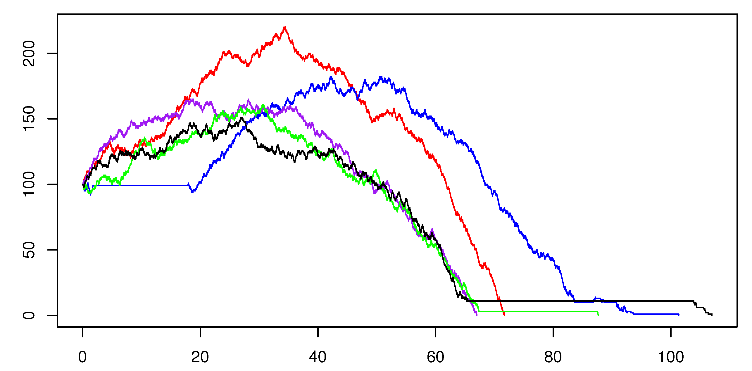For other Bernstein functions, one could provide simulation procedures for random variables with distribution $1-{\mathfrak{e}}_{\mathsf{\Phi }}(t;-\lambda )$ by using the fact that the Laplace transform is known (see [59]). In Figure 5, different simulated paths of the process $I^{\mathsf{\Phi }}\left(t\right)$ are represented, all for $I_0=100$ (and $S_0=900$), $\beta =1.5/S_0$, and $\gamma =1$ (in such a way that ${\mathcal{R}}_0=1.5$). As one can see, the sojourn times vary in length in such a way to produce some actually long constancy intervals. Let us indeed recall that, despite being almost surely finite, the sojourn times admit infinite mean, thus we can expect long sojourn times with non-negligible probability (even more in the case $\mathsf{\Phi }\left(\lambda \right)={\lambda }^{\alpha }$, since we know that $E_{\alpha }(-\lambda t^{\alpha })$ decays as $t^{-\alpha }$ and then the sojourn times admit a power-law decay).

Figure 5. Plots of simulated trajectories of $I^{\mathsf{\Phi }}\left(t\right)$, with $\mathsf{\Phi }\left(\lambda \right)={\lambda }^{\alpha }$, $I_0=100$, $S_0=900$, $\gamma =1$, $\beta =1.5/S_0$, and $\alpha =0.7$. The discretization time interval is given by $\delta t=0.05$.

In Figure 6, we represent the trajectories of $t\mapsto \frac{(\mathbb{E}\left[S_{\mathsf{\Phi }}\left(t\right)\right],\mathbb{E}\left[I_{\mathsf{\Phi }}\left(t\right)\right])}{N}$ for $N=1000$, $\alpha =0.7$, $\gamma =1$, and $\beta =2/N$, varying the values of $S_0$ and $I_0$. We obtain something that reminds of the phase portraits in Figure 3.

Figure 6. Phase portrait of $\frac{(\mathbb{E}\left[S_{\mathsf{\Phi }}\left(t\right)\right],\mathbb{E}\left[I_{\mathsf{\Phi }}\left(t\right)\right])}{N}$ as $N=1000$, $\alpha =0.7$, $\gamma =1,$ and $\beta =2/N$. The time interval $t\in [0,T]$ is obtained by $T=(N_{max}+1)\delta t$ where $N_{max}=2000$ and $\delta t=500N^{\frac{1}{\alpha }}$. The expectations are approximated by means of averages of $N_{traj}=1000$ simulated sample paths of $S_{\mathsf{\Phi }}\left(t\right)$ and $I_{\mathsf{\Phi }}\left(t\right)$ with discretization time interval $\delta t=500N^{\frac{1}{\alpha }}$.

Even though the shapes of the phase portraits are similar, the dynamics happen in different time-scales, as one can see in Figure 7.

Figure 7. In red, the plot of $I^{\mathsf{\Phi }}\left(t\right)$ for $\gamma =1$, $\beta =2$, $\alpha =0.7$, and $I_0=0.3$. In blue, the plot of $\frac{\mathbb{E}\left[I_{\mathsf{\Phi }}\left(t\right)\right]}{N}$ for $\gamma =1$, $N=1000$, $\beta =2/N$, $\alpha =0.7,$ and $I_0=300$. For both plots, the discretization time interval is given by $\delta t=0.05$. The expected value $\mathbb{E}\left[I_{\mathsf{\Phi }}\left(t\right)\right]$ is approximated by means of the average of $N_{traj}=1000$ simulated sample paths.

Indeed, we show above that the large population limit of the time-changed continuous time Markov chain does not coincide with the solution of the non-local dynamical system (7). Numerical evidence of this loss of fluid limit is given in Table 1. Here, for a fixed time horizon $T>0$, we consider the error function

$$E_T\left(N\right)=\underset{t\in [0,T]}{sup}\sqrt{{(I^{\mathsf{\Phi }}\left(t\right)-\mathbb{E}\left[I_{\mathsf{\Phi }}\left(t\right)\right])}^2+{(S^{\mathsf{\Phi }}\left(t\right)-\mathbb{E}\left[S_{\mathsf{\Phi }}\left(t\right)\right])}^2}.$$

Table 1. The values of $E_T\left(N\right)$ as N varies for different values of $\alpha$, $T=10$, $I_0=0.1$, and $S_0=0.9$ for the deterministic case (while for the stochastic one $I_0=0.1N$ and $S_0=0.9N$), as well as $\gamma =1$ and $\beta =2$ for the deterministic case (while for the stochastic one $\beta =2/N$). The discretization time interval is given by $\delta t=0.05$.

$\alpha =0.9$	N	1000	5000	10,000	50,000	100,000	500,000
	$E_T\left(N\right)$	$0.5668881$	$0.6279486$	$0.6370400$	$0.6448136$	$0.6458144$	$0.6466264$
$\alpha =0.8$	N	1000	5000	10,000	50,000	100,000	500,000
	$E_T\left(N\right)$	$0.5011228$	$0.5620085$	$0.5716072$	$0.5799426$	$0.5810315$	$0.5819122$
$\alpha =0.7$	N	1000	5000	10,000	50,000	100,000	500,000
	$E_T\left(N\right)$	$0.4457108$	$0.5088696$	$0.5201510$	$0.5299119$	$0.5311337$	$0.5321171$
$\alpha =0.6$	N	1000	5000	10,000	50,000	100,000	500,000
	$E_T\left(N\right)$	$0.3960360$	$0.4640787$	$0.4762837$	$0.4861995$	$0.4874512$	$0.4884569$
$\alpha =0.5$	N	1000	5000	10,000	50,000	100,000	500,000
	$E_T\left(N\right)$	$0.3527517$	$0.4218395$	$0.4341420$	$0.4442546$	$0.4455378$	$0.4465600$

8. Conclusions

Let us summarize here the main results and some observations that follow from them. In Section 3, we introduce a non-local generalization of the SIR model by simply substituting the classical derivative with a Caputo-type derivative. Despite the naive substitution, this new model exhibits some features that are more complicated to study. We are able to recover (in some form) the ${\mathcal{R}}_0$-dogma. However, the lack of semigroup property leads to some unexpected results. We do not have any sufficient condition for monotonicity of functions by knowing the sign of their Caputo-type derivative. The lack of such sufficient condition can also be seen from the phase portrait in Figure 3, as the maximum is reached in a region in which $\frac{d^{\mathsf{\Phi }}{I}^{\mathsf{\Phi }}}{d{t}^{\mathsf{\Phi }}}$ is still strictly positive. Let us indeed recall that the classical Fermat theorem on extremal points (see, e.g., [60] Theorem $5.9$) becomes an inequality in the non-local context (see, e.g., [61] Theorem 1 in the fractional case or [62] Proposition 2.2 in the general Caputo-type case), justifying the fact that, after the function reaches a maximum and starts decreasing, the non-local derivative could still be non-negative. Finally, let us observe that the lack of semigroup property can be overtaken by considering a deformation map $\theta$, as shown in Appendix A, that takes in consideration the fact that the system remembers all its history.

On the other hand, in Section 5, we study the properties of a time-changed stochastic SIR model. In the linear context, time-changed processes provide the direct non-local counterpart of their parent process, as one can see, for instance, in [22,23,24,25,63,64], and many others. In the non-linear context, as for the SIR model, things can go differently. Indeed, even in the classical case, the equation of the expected value is affected by the non-linearity that appears as the covariance between the two components of the process. However, in the Markov case, we still have a fluid limit that links the deterministic case with the mean field dynamics of the stochastic case. In the time-changed case, this does not happen, as shown in Section 6. Thus, even though the time-changed SIR model preserves all the properties of the stationary state of the parent model and its forward Kolmogorov equations can be obtained from the parent’s one by considering a Caputo-type derivative in place of the classical one, the whole model cannot be directly seen as the stochastic counterpart of the non-local SIR model introduced in Section 3. All these observations and statements are then supported by numerical evidence, as shown in Section 7.

Finally, concerning modeling purposes, let us observe that the time-changed SIR model should be used only to model subdiffusive epidemics. Indeed, one could use a continuous mapping approach to prove that Löf’s diffusive approximation of the classical stochastic SIR model (see [5] and references therein) leads to a subdiffusive approximation of the time-changed SIR model. Thus, when working with time-changed models (including also fractional ones), one should always take in consideration the fact that such models exhibit an approximatively subdiffusive behavior and then should be used only in contextualization of such behavior with empirical evidence.