Heating a 2D Thermoelastic Half-Space Induced by Volumetric Absorption of a Laser Radiation

Abstract

In this work, the generalized theory with dual-phase-lag of thermoelasticity is employed to study the influences induced by absorbing a penetrating laser radiation inside a 2D thermoelastic semi-infinite medium. The medium’s surface is presumed to be exposed to temperature-dependent heat losses and is traction-free. The considered problem is solved using the integral transforms technique by applying the double-transformation Laplace and Hankel. A numerical fashion is applied to obtain the inverse of the Laplace transformation. The results of this problem are presented graphically for some studied fields.

1. Introduction

One of the celebrated contributions to the field of thermoelasticity is the coupled theory, which was formulated by Biot in 1956 [1], in which the author tackled one of the faults of the classical uncoupled theory of thermoelasticity by modifying the energy equation to contain a term representing the strain field. Since Biot’s model was based upon Fourier’s law, it failed to address the second defect of the classical uncoupled theory, which means that the generated heat waves still propagate with an infinite velocity. Hence, the behavior of Biot’s theory contradicts the laws of physics, especially for some problems such as utilizing laser heat sources, where their pulse duration is extremely short, and problems with large temperature gradients [2,3].

After Biot’s attempt, great efforts were made to obtain a generalization that addressed the defect found in the coupled theory; this point became the focus of attention for those interested in thermoelasticity. Authentic progress was made in 1967 when Lord and Shulman [4] formulated a new model based on Cattaneo’s approach [5,6] instead of Fourier’s Law. This theory was followed by several essential generalizations [7,8,9]; most of these theories were dependent on adjusting the heat equation. The DPL model or the generalized theory with dual-phase-lag is one of the essential generalizations developed by Tzou [10,11], where the energy equation was modified to contain two distinct phase-lags: one symbolizes the temperature gradient, while the other symbolizes the heat flux. Several authors have employed the DPL model to study thermoelastic waves under the effect of different fields [12,13,14,15,16,17,18,19].

Since the discovery of lasers, many applications in physics, mechanics, and engineering have been implemented based on their various properties, especially in materials processing, such as drilling of holes, spot welding, glazing of materials, and surface-hardening scribing [20]. Several authors have employed the generalized theories of thermoelasticity to study the thermoelastic interactions induced by a pulsed laser, considering different aspects [21,22,23,24]. Zenkour and Aboelregal [25] studied the fractional influences in a half-space solid exposed to non-Gaussian laser radiation by utilizing the two-temperature generalized model with a fractional-order energy equation. Bassiouny et al. [26] investigated the thermoelastic conduct of an elastic semi-infinite solid under the influence of a pulsed laser, by applying the theory of fractional-order strain thermoelasticity. Allam and Tayel [27] applied five different theories to study the interaction caused by surface absorption of a pulsed laser in a functionally graded thermoelastic semi-infinite medium. Abbas and Marin [28] employed the Lord and Shulman model to study the effect of the relaxation time in a 2D thermoelastic semi-infinite solid illuminated by a laser pulse. Abouelregal and Zenkour [29] employed the generalized two-temperature thermoelastic theory to discuss thermoelastic responses in a half-space, whose pounding plane was exposed to a laser pulse. Tayel and Hassan [30] and Tayel [31] studied the thermoelastic interaction induced by both surface and volumetric absorption techniques, respectively, in a one-dimensional semi-infinite medium, considering the absence and existence of cooling, by employing various thermoelasticity theories.

Integral transforms have been effectively employed for solving many problems in physics, applied mathematics, and engineering sciences. Although Laplace transform is considered one of the most essential integral transformations applied to solve coupling problems in the theory of thermoelasticity, its inverse is very difficult to obtain using the usual methods. This difficulty has prompted those interested in thermoelasticity to apply numerical methods or to use asymptotic expansion techniques that are adequate for short times. This technique was used in the context of the coupled theory by Hetnarski [32,33] and applied by several authors to some generalized thermoelastic problems [34,35,36].

The main goals of this work are to study the thermoelastic interaction induced by the volumetric absorption technique of a laser pulse in a 2D semi-infinite medium and to investigate the effects of the phase-lag parameters of the DPL theory of thermoelasticity on the existence and absence of a cooling effect. The medium is studied under the influence of a laser beam, the spatial and temporal profiles of which are considered Gaussian. The medium surface is exposed to temperature-dependent heat losses and is considered traction-free.

2. Problem Formulation

A thermoelastic, isotropic, and homogeneous 2D semi-infinite medium $\left(z\ge 0\right)$ is considered under the influence of a laser beam that is incident-normal to a small specified region of the medium’s surface. The medium is initially at a uniform temperature $T_0$ and its surface $\left(z=0\right)$ is taken as stress-free and assumed to be exposed to temperature-dependent cooling. The cylindrical coordinate system $\left(r, \varphi , z\right)$ is utilized in the problem, with the z-axis oriented inward and vertically.

According to the heating process, which is considered axisymmetric, all quantities will depend on $r$, $z$ and $t$ only and, thus, the displacement vector $u$ will possess the following components:

$$u_r=u\left(r, z, t\right), u_{\varphi }=0, u_z=w\left(r, z, t\right).$$

(1)

Consequently, the nonvanishing strain components are

$$e_{rr}= \frac{\partial u}{\partial r}, e_{zz}=\frac{\partial w}{\partial z}, e_{\varphi \varphi }= \frac{u}{r} , e_{rz}=\frac{1}{2}\left(\frac{\partial u}{\partial z}+\frac{\partial w}{\partial r}\right).$$

Thus, the dilatation $e$ takes the form

$$e=e_{rr}+e_{\varphi \varphi }+e_{zz}=\frac{1}{r}\frac{\partial }{\partial r}(r u)+\frac{\partial w}{\partial z}.$$

(2)

Following [10,11], the linear heat equation for a homogeneous and isotropic body in the context of the DPL model is given as

$$\begin{gathered} k \left(1+{\tau }_1\frac{\partial }{\partial t}\right){\nabla }^{2}T= \left(1+{\tau }_2\frac{\partial }{\partial t}+\frac{{\tau }_2^2}{2}\frac{{\partial }^2}{\partial t^2}\right)\left(\rho C_E \frac{\partial T}{\partial t}+\gamma T_0 \frac{\partial e}{\partial t}-Q\left(r,z,t\right)\right) , \\ \mathrm{with} {\nabla }^2(•)=\left(\frac{{\partial }^2}{\partial r^2}+\frac{1}{r}\frac{\partial }{\partial r}+\frac{{\partial }^2}{\partial z^2}\right)(•), \end{gathered}$$

(3)

where $k$ stands for thermal conductivity; $\rho$ for density; $T$ for the absolute temperature, $C_E$, for the specific heat at constant strain; $T_0$ for the reference temperature, which is chosen such that $\left|\left(T-T_0\right)/T_0\right|\ll 1$ and ${\tau }_1$, ${\tau }_2$ for phase-lags of the temperature gradient and the heat flux, respectively, where $\left({\tau }_1,{\tau }_2>0\right)$. Moreover, $\gamma =\left(3\lambda +2\mu \right){\alpha }_T$, in which $\lambda$ and $\mu$ are lamé’s constants and ${\alpha }_T$ is the thermal expansion.

For volumetric absorption in a 2D medium, $Q \left(r,z,t\right)$ is given as

$$Q \left(r,z,t\right)=A_0{q}_{0}Q\left(t\right) e^{\frac{-r^2}{{\omega }^2}}\beta e^{-\beta z} ,$$

(4)

where $A_0, q_0,Q\left(t\right),\omega ,\beta$ denote the transition coefficient of the illuminated surface, the maximum value of the laser intensity, the temporal laser pulse shape, a spatial constant, and the absorption coefficient of the material, respectively.

The axially symmetric equations of motion in terms of displacements and absence of body forces are

$$\left(\lambda +\mu \right)\frac{\partial e}{\partial r}+\mu \left({\nabla }^2-\frac{1}{r^2}\right)u-\gamma \frac{\partial T}{\partial r}=\rho \frac{{\partial }^{2}u}{\partial t^2},$$

(5)

$$\left(\lambda +\mu \right) \frac{\partial e}{\partial z}+\mu {\nabla }^2 w-\gamma \frac{\partial T}{\partial z}=\rho \frac{{\partial }^{2}w}{\partial t^2}.$$

(6)

Furthermore, the nonvanishing stresses are determined by

$${\sigma }_{zz}=2\mu \frac{\partial w}{\partial z}+\lambda e-\gamma \theta ,$$

(7)

$${\sigma }_{rr}=2\mu \frac{\partial u}{\partial r}+\lambda e-\gamma \theta ,$$

(8)

$${\sigma }_{\varphi \varphi }=2\mu \frac{u}{r}+\lambda e-\gamma \theta ,$$

(9)

$${\sigma }_{rz}=\mu \left(\frac{\partial u}{\partial z}+\frac{\partial w}{\partial r}\right),$$

(10)

where $\theta =T-T_0$ represents the increment of the temperature.

Due to the foregoing formulation, the boundary conditions will be

$$\begin{array}{l}{{{\sigma }_{zz}|}_{z=0}={\sigma }_{rz}|}_{z=0}=0,\\ k\left(1+{\tau }_1\frac{\partial }{\partial t}\right) {\frac{\partial \theta }{\partial z}|}_{z=0}= \left(1+{\tau }_2\frac{\partial }{\partial t}+\frac{{\tau }_2^2}{2}\frac{{\partial }^2}{\partial t^2}\right)h \theta \left(r,0,t\right),\end{array}\}$$

(11)

where $h$ represents the coefficient of the heat transfer responsible for cooling, and $\theta \left(r,0,t\right)$ is the surface temperature.

Additionally, the initial conditions are

$$\begin{array}{l}{\theta (r,z,t)|}_{t=0}={\frac{\partial \theta (r,z,t)}{\partial t}|}_{t=0}=0, {u(r,z,t)|}_{t=0}={\frac{\partial u(r,z,t)}{\partial t}|}_{t=0}=0,\\ {w(r,z,t)|}_{t=0}={\frac{\partial w(r,z,t)}{\partial t}|}_{t=0}=0.\end{array}\}$$

(12)

Now, we introduce the following nondimensional variables

$$\begin{gathered} \left(u^{\prime },w^{\prime }, r^{\prime },z^{\prime }, {\omega }^{\prime }\right)=c \eta \left(u,w, r,z,\omega \right)\hspace{1em}{\theta }^{\prime }=\frac{\gamma \theta }{\left(\lambda +2\mu \right)}\hspace{1em}{{\sigma }^{\prime }}_{ij}=\frac{{\sigma }_{ij}}{\mu } \\ \left(t^{\prime },{{\tau }^{\prime }}_1, {{\tau }^{\prime }}_2\right)=c^2\eta \left(t,{\tau }_1, {\tau }_2\right)\hspace{1em}{h}^{\prime }=\frac{h}{c \rho C_E}\hspace{1em}{\beta }^{\prime }=\frac{\beta }{c \eta } \\ {q^{\prime }}_0=\frac{\gamma q_0}{\left(\lambda +2\mu \right)c \rho C_E} \end{gathered}$$

(13)

where $c^2=\frac{\lambda +2\mu }{\rho }$, $\eta =\frac{\rho c_E }{k}$.

For seeking the simplicity primes will be dropped, and thus Equations (3), (5) and (6) in the nondimensional forms will be

$$\left(1+{\tau }_1\frac{\partial }{\partial t}\right) {\nabla }^2\theta =\left(1+{\tau }_2\frac{\partial }{\partial t}+\frac{{\tau }_2^2}{2}\frac{{\partial }^2}{\partial t^2}\right)\left(\frac{\partial \theta }{\partial t}+\epsilon \frac{\partial e}{\partial t}-A_0{q}_0\beta Q\left(t\right)e^{-\frac{r^2}{{\omega }^2}}{e}^{-\beta z}\right),$$

(14)

$$\left(g - 1\right)\frac{\partial e}{\partial r}+\left({\nabla }^2 -\frac{1}{r^2}\right)u-g\frac{\partial \theta }{\partial r}=g\frac{{\partial }^{2}u}{\partial t^2},$$

(15)

$$\left(g - 1\right)\frac{\partial e}{\partial z}+{\nabla }^{2}w-g\frac{\partial \theta }{\partial z}=g\frac{{\partial }^{2}w}{\partial t^2},$$

(16)

where $g=\frac{\lambda +2\mu }{\mu }$, $\epsilon =\frac{T_0{\gamma }^2}{\rho C_E(\lambda +2\mu )}$.

Combining Equations (15) and (16) by applying the operators $\frac{1}{r}\left(\frac{\partial }{\partial r}r.\right)$ for (15) and $\frac{\partial }{\partial z}$ for (16), then adding them, one gets

$${\nabla }^{2}e-{\nabla }^2\theta =\frac{{\partial }^{2}e}{\partial t^2}.$$

(17)

In the nondimensional form, the stress components become

$${\sigma }_{rr}=2\frac{\partial u}{\partial r}+\left(g-2\right)e-g\theta ,$$

(18)

$${\sigma }_{zz}=2\frac{\partial w}{\partial z}+\left(g-2\right)e-g\theta ,$$

(19)

$${\sigma }_{\varphi \varphi }=2\frac{u}{r}+\left(g-2\right)e-g\theta ,$$

(20)

$${\sigma }_{rz}=\frac{\partial u}{\partial z}+\frac{\partial w}{\partial r}.$$

(21)

In addition, Equation (11) will be written as

$$\begin{array}{l}{\left({\sigma }_{zz}={\sigma }_{rz}\right)|}_{z=0}=0,\\ \left(1+{\tau }_1\frac{\partial }{\partial t}\right){\frac{\partial \theta }{\partial z}|}_{z=0}=\left(1+{\tau }_2\frac{\partial }{\partial t} + \frac{{\tau }_2^2}{2} \frac{{\partial }^2}{\partial t^2}\right) h \theta \left(r,0,t\right).\end{array}\}$$

(22)

3. Problem Solution

The specific conditions in Equation (12) and the basic Equations (14) and (17) predict that the double-transformation Laplace and Hankel integral transforms [37] are more appropriate to be applied for $t$ and $r$, respectively, in which the transformation is given as

$$\begin{array}{l}\tilde{\overline{f}}\left( \alpha , z, s\right)={\displaystyle \underset{0}{\overset{\infty }{\int }}{\displaystyle \underset{0}{\overset{\infty }{\int }}r{J}_n\left(\alpha r\right)f\left(r,z,t\right)} e^{-st}dr d t,}\\ f\left(r,z,t\right)=\frac{1}{2\pi i} {\displaystyle \underset{\sigma -i \infty }{\overset{\sigma +i \infty }{\int }}{\displaystyle \underset{0}{\overset{\infty }{\int }}\alpha J_n\left(\alpha r\right)\tilde{\overline{f}}\left(\alpha ,z,s\right)e^{st}d \alpha d s,}}\end{array}\}$$

(23)

where $s$ is the Laplace transform variable, the superscripts dash and tilde indicate the Laplace and Hankel transformation of $f\left(r,z,t\right)$, respectively, and $J_n$ is the Bessel function of the first kind of order $n$ in which

$$n=\{\begin{array}{l}0\hspace{1em}\hspace{1em}\mathrm{for} \overline{f}\left(r, z, s\right)= \left\{\overline{\theta }, \overline{w}, \overline{e}, {\overline{\sigma }}_{zz}, {\overline{\sigma }}_{rr}, {\overline{\sigma }}_{\varphi \varphi }\right\}\left(r, z, s\right)\\ 1\hspace{1em}\hspace{1em}\mathrm{for} \overline{f}\left(r, z, s\right)= \left\{\overline{u}, {\overline{\sigma }}_{rz}\right\}\left(r, z, s\right) \end{array} .$$

Thus, Equations (14) and (17) become, respectively

$$\left(D^2-{\alpha }^2-s \mathsf{\Gamma }\right)\tilde{\overline{\theta }}-\epsilon s \mathsf{\Gamma } \tilde{\overline{e}}=-A_0{q}_0\beta \mathsf{\Gamma }\overline{Q}\left(s\right)\tilde{\eta }\left(\alpha \right)e^{-\beta z}.$$

(24)

$$\left(D^2-{\alpha }^2-s^2\right)\tilde{\overline{e}}-\left(D^2-{\alpha }^2\right)\tilde{\overline{\theta }}=0,$$

(25)

where $\mathsf{\Gamma }=\frac{1+{\tau }_{2}s+\frac{{\tau }_2^2}{2}{s}^2}{1+{\tau }_{1}s},$ $\overline{Q}(s)$ is the Laplace transform of $Q(t)$, and $\tilde{\eta }\left(\alpha \right)=\frac{{\omega }^2}{2}{e}^{-\frac{1}{4}{\alpha }^2{\omega }^2}$ is the Hankel transform of order zero of $e^{\frac{-r^2}{{\omega }^2}}$.

The elimination of $\tilde{\overline{e}}$ between Equations (24) and (25) gives

$$\left(D^4-b_1\left(\alpha ,s\right)D^2+b_2\left(\alpha ,s\right)\right)\tilde{\overline{\theta }}=-A_0{q}_0\beta \mathsf{\Gamma }\left({\beta }^2-{\alpha }^2-s^2\right)\overline{Q}\left(s\right)\tilde{\eta }\left(\alpha \right)e^{-\beta z},$$

(26)

where $b_1\left(\alpha ,s\right)=2{\alpha }^2+s^2+s\mathsf{\Gamma }\left(1+\epsilon \right)$, $b_2\left(\alpha ,s\right)={\alpha }^4+{\alpha }^2{s}^2+s\mathsf{\Gamma }{\alpha }^2\left(1+\epsilon \right) +s^3\mathsf{\Gamma }$.

Consequently, Equation (26) can be written as

$$\left(D^2-k_1^2\right)\left(D^2-k_2^2\right)\tilde{\overline{\theta }}=-A_0{q}_0\beta \mathsf{\Gamma }\left({\beta }^2-{\alpha }^2-s^2\right)\overline{Q}\left(s\right)\tilde{\eta }\left(\alpha \right)e^{-\beta z}.$$

(27)

where $k_i^2$ are the roots of the following auxiliary equation:

$$k^4-b_1\left(\alpha ,s\right)k^2+b_2\left(\alpha ,s\right)=0.$$

(28)

The solution of Equation (27) after considering the behavior of $\tilde{\overline{\theta }}$ as $z\to \infty$ is given as

$$\tilde{\overline{\theta }}\left(\alpha ,z,s\right)={\displaystyle \sum _{i=1}^2{B}_i(\alpha ,s) e^{-k_{i}z}+M\left(\alpha ,s\right)e^{-\beta z}},$$

(29)

where $M\left(\alpha ,s\right)$ represents the coefficient of the particular solution of Equation (27); using the undetermined coefficients method, one gets

$$M\left(\alpha ,s\right)=-\frac{A_0{q}_0\mathsf{\Gamma }\beta \left({\beta }^2-{\alpha }^2-s^2\right)\overline{Q}\left(s\right)\tilde{\eta }\left(\alpha \right)}{\left({\beta }^2-k_1^2\right)\left({\beta }^2-k_2^2\right)},$$

(30)

and thus

$$\tilde{\overline{\theta }}\left(\alpha ,z,s\right)={\displaystyle \sum _{i=1}^2{B}_i(\alpha ,s) e^{-k_{i}z}-\frac{A_0{q}_0\mathsf{\Gamma }\beta \left({\beta }^2-{\alpha }^2-s^2\right)\overline{Q}\left(s\right)\tilde{\eta }\left(\alpha \right)}{\left({\beta }^2-k_1^2\right)\left({\beta }^2-k_2^2\right)}{e}^{-\beta z}}.$$

(31)

In a similar fashion, the elimination of $\tilde{\overline{\theta }}$ between Equations (24) and (25) gives

$$\left(D^2-k_1^2\right)\left(D^2-k_2^2\right)\tilde{\overline{e}}=-A_0{q}_0\beta \mathsf{\Gamma }\left({\beta }^2-{\alpha }^2\right)\overline{Q}\left(s\right)\tilde{\eta }\left(\alpha \right)e^{-\beta z}.$$

(32)

Solving (32), one can obtain

$$\tilde{\overline{e}}\left(\alpha ,z,s\right)={\displaystyle \sum _{i=1}^2{E}_i{e}^{-k_{i}z}+e_p\left(\alpha ,s\right)e^{-\beta z}},$$

(33)

where $e_p$ is the coefficient of the particular solution of (32).

$$e_p=-\frac{A_0{q}_0\mathsf{\Gamma }\beta \left({\beta }^2-{\alpha }^2\right)\overline{Q}\left(s\right)\tilde{\eta }\left(\alpha \right)}{\left({\beta }^2-k_1^2\right)\left({\beta }^2-k_2^2\right)}.$$

(34)

Introducing Equations (29) and (33) into Equation (25) yields

$$E_i(\alpha ,s)=\left(\frac{k_i^2-{\alpha }^2}{k_i^2-{\alpha }^2-s^2}\right)B_i(\alpha ,s),$$

(35)

$$e_p\left(\alpha ,s\right)=\left(\frac{{\beta }^2-{\alpha }^2}{{\beta }^2-{\alpha }^2-s^2}\right)M\left(\alpha ,s\right),$$

(36)

So that

$$\tilde{\overline{e}}={\displaystyle \sum _{i=1}^2\left(\frac{k_i^2-{\alpha }^2}{k_i^2-{\alpha }^2-s^2}\right)B_i{e}^{-k_{i}z}-}\frac{A_0{q}_0\mathsf{\Gamma }\beta \left({\beta }^2-{\alpha }^2\right)\overline{Q}\left(s\right)\tilde{\eta }\left(\alpha \right)}{\left({\beta }^2-k_1^2\right)\left({\beta }^2-k_2^2\right)}{e}^{-\beta z}.$$

(37)

Applying (23) to Equation (16), one gets

$$(D^2-{\alpha }^2-g s^2) \tilde{\overline{w}}=gD \tilde{\overline{\theta }}-(g-1)D \tilde{\overline{e}}.$$

(38)

Substituting for $\tilde{\overline{\theta }}$ and $\tilde{\overline{e}}$ in Equation (38), then solving the nonhomogeneous second-order ordinary differential equation, this gives

$$\tilde{\overline{w}}=N\left(\alpha ,s\right)e^{-\xi z}-{\displaystyle \sum _{i=1}^2\left(\frac{k_i}{k_i^2-{\alpha }^2-s^2}\right)B_i\left(\alpha ,s\right)e^{-k_{i}z}} +\frac{A_0{q}_0\mathsf{\Gamma }{\beta }^2\overline{Q}\left(s\right)\tilde{\eta }\left(\alpha \right)}{\left({\beta }^2-k_1^2\right)\left({\beta }^2-k_2^2\right)}{e}^{-\beta z},$$

(39)

where $\xi =\sqrt{{\alpha }^2+g s^2}$.

Applying (23) on the nondimensional form of Equation (2) and making use of the relation $H_n\left\{r^{-n-1}\frac{d}{dr}\left(r^{1+n}\overline{f}\left(r,z,s\right)\right)\right\}=\alpha H_{n+1}\left\{\overline{f}\left(r,z,s\right)\right\}$ for $n=0,$ it follows

$$\tilde{\overline{e}}=\alpha \tilde{\overline{u}}+\frac{d \tilde{\overline{w}}}{d z},$$

(40)

where $H_n\left\{f\left(r\right)\right\}$ represents the Hankel transform of $f\left(r\right)$.

Now, in order to obtain $\tilde{\overline{u}}$, we shall substitute Equations (37) and (39) into Equation (40); one gets

$$\tilde{\overline{u}}=\frac{1}{\alpha }\left(\xi N{e}^{-\xi z}-{\displaystyle \sum _{i=1}^2\left(\frac{{\alpha }^2}{k_i^2-{\alpha }^2-s^2}\right)B_i{e}^{-k_{i}z}+\frac{A_0{q}_0\mathsf{\Gamma }\beta {\alpha }^2\overline{Q}\left(s\right)\tilde{\eta }\left(\alpha \right)}{\left({\beta }^2-k_1^2\right)\left({\beta }^2-k_2^2\right)}{e}^{-\beta z}}\right).$$

(41)

The stress components of the problem can be obtained by applying (23) on (18), (19), (20) and (21); this gives the following relations:

$${\tilde{\overline{\sigma }}}_{rr}=-2\alpha \tilde{\overline{u}}+\left(g-2\right)\tilde{\overline{e}}-g\tilde{\overline{\theta }},$$

(42)

$${\tilde{\overline{\sigma }}}_{zz}=2\frac{d \tilde{\overline{w}}}{dz}+\left(g-2\right)\tilde{\overline{e}}-g\tilde{\overline{\theta }},$$

(43)

$${\tilde{\overline{\sigma }}}_{\varphi \varphi }=2\alpha \tilde{\overline{u}}+\left(g-2\right)\tilde{\overline{e}}-g\tilde{\overline{\theta }},$$

(44)

$${\tilde{\overline{\sigma }}}_{rz}=\frac{d \tilde{\overline{u}}}{dz}-\alpha \tilde{\overline{w}}.$$

(45)

From the stresses above, only the stresses that related to the boundary conditions will be picked out to be calculated; hence, introducing Equations (31), (37), (39), and (41) into (43) and (45), it follows

$${\tilde{\overline{\sigma }}}_{zz}=-2\xi N{e}^{-\xi z}+{\displaystyle \sum _{i=1}^2\left(\frac{\mathsf{\Omega }}{k_i^2-{\alpha }^2-s^2}\right)} B_i{e}^{-k_{i}z} -\frac{A_0{q}_0\mathsf{\Gamma }\beta \mathsf{\Omega } \overline{Q}\left(s\right)\tilde{\eta }\left(\alpha \right)}{\left({\beta }^2-k_1^2\right)\left({\beta }^2-k_2^2\right)}{e}^{-\beta z},$$

(46)

$${\tilde{\overline{\sigma }}}_{rz}=\frac{1}{\alpha }\left(-\mathsf{\Omega } N{e}^{-\xi z}+{\displaystyle \sum _{i=1}^2\left(\frac{2{\alpha }^2{k}_i}{k_i^2-{\alpha }^2-s^2}\right)} B_i{e}^{-k_{i}z} -\frac{2A_0{q}_0\mathsf{\Gamma }{\beta }^2{\alpha }^2 \overline{Q}\left(s\right)\tilde{\eta }\left(\alpha \right)}{\left({\beta }^2-k_1^2\right)\left({\beta }^2-k_2^2\right)}{e}^{-\beta z}\right).$$

(47)

where $\mathsf{\Omega }=2{\alpha }^2+g s^2.$

Now making use of Equations (31), (46), and (47), Equations (22) can be written as

$$-{\displaystyle \sum _{i=1}^2{k}_i B_i\left(\alpha ,s\right)=} M_1+\mathsf{\Gamma } h \tilde{\overline{\theta }}\left(\alpha ,0,s\right),$$

(48)

$${\displaystyle \sum _{i=1}^2{F}_i B_i\left(\alpha ,s\right)-2 \xi N\left(\alpha ,s\right)=}{M}_2,$$

(49)

$${\displaystyle \sum _{i=1}^2{F}_{i+2} B_i\left(\alpha ,s\right)- \mathsf{\Omega } N\left(\alpha ,s\right)=} M_3,$$

(50)

where

$$\begin{array}{l}{M}_1=\beta M, M_2= -\frac{\mathsf{\Omega } M}{\left({\beta }^2-{\alpha }^2-s^2\right)}, M_3=-\frac{2\beta {\alpha }^{2}M}{\left({\beta }^2-{\alpha }^2-s^2\right)},\\ F_i=\left(\frac{\mathsf{\Omega }}{k_i^2-{\alpha }^2-s^2}\right), F_{i+2}=\left(\frac{2{\alpha }^2{k}_i}{k_i^2-{\alpha }^2-s^2}\right), \left(i=1,2\right).\end{array}$$

Solving (48), (49), and (50), one gets

$$B_1=\frac{\left(h \mathsf{\Gamma }\tilde{\overline{\theta }}\left(\alpha , 0, s\right)+M_1\right)\left(2\xi F_4- \mathsf{\Omega } F_2\right)+\left(2 \xi M_3-\mathsf{\Omega } M_2\right)k_2}{\left(\mathsf{\Omega } F_2-2\xi F_4\right)k_1+\left(2\xi F_3-\mathsf{\Omega } F_1\right)k_2},$$

(51)

$$B_2=\frac{\left(h \mathsf{\Gamma }\tilde{\overline{\theta }}\left(\alpha , 0, s\right)+M_1\right)\left(\mathsf{\Omega } F_1-2\xi F_3\right)+\left(\mathsf{\Omega } M_2-2 \xi M_3\right)k_1}{\left(\mathsf{\Omega } F_2-2\xi F_4\right)k_1+\left(2\xi F_3-\mathsf{\Omega } F_1\right)k_2},$$

(52)

$$N=\frac{\left(F_4{k}_1-F_3{k}_2\right)M_2+\left(h \mathsf{\Gamma }\tilde{\overline{\theta }}\left(\alpha , 0, s\right)+M_1\right)\left(F_1{F}_4-F_2{F}_3\right)+\left(F_1{k}_2-F_2{k}_1\right)M_3}{\left(\mathsf{\Omega } F_2-2\xi F_4\right)k_1+\left(2\xi F_3-\mathsf{\Omega } F_1\right)k_2}.$$

(53)

Substituting Equations (51)–(53) into Equation (31) and setting $\left(z=0\right)$, this gives the surface temperature $\tilde{\overline{\theta }}\left(\alpha ,0,s\right)$ as follows:

$$\tilde{\overline{\theta }}\left(\alpha ,0,s\right)=\frac{M_1 \left(\left(2\xi F_3-\mathsf{\Omega } F_1\right)\left(\beta +k_2\right)+\left(\mathsf{\Omega } F_2 -2\xi F_4\right)\left(\beta +k_1\right)\right)+\beta \left(k_1-k_2\right)\left(-\mathsf{\Omega } M_2+2 \xi M_3\right)}{\beta \left(\left(2F_4 \xi -F_2 \mathsf{\Omega }\right)\left(h\mathsf{\Gamma }+k_1\right)+\left(F_1 \mathsf{\Omega }-2F_3 \xi \right)\left(h\mathsf{\Gamma }+k_2\right)\right)}.$$

(54)

4. Small Time Approximation

The above calculations and the roots of the auxiliary Equation (28) foretell that converting the solution to the physical domain is too difficult to be performed using the usual methods. So, a small time approximation will be adapted for the roots, conforming to great s-values; this technique was used in [36] according to [38,39].

The roots of Equation (28) are given as

$$k_1=\frac{\sqrt{2{\alpha }^2+s^2+s\mathsf{\Gamma } \left(\epsilon +1\right)+s \sqrt{s^2+2s\mathsf{\Gamma } \left(\epsilon -1\right)+{\mathsf{\Gamma }}^2{\left(\epsilon +1\right)}^2}}}{\sqrt{2}},$$

(55)

$$k_2=\frac{\sqrt{2{\alpha }^2+s^2+s\mathsf{\Gamma } \left(\epsilon +1\right)-s \sqrt{s^2+2s\mathsf{\Gamma } \left(\epsilon -1\right)+{\mathsf{\Gamma }}^2{\left(\epsilon +1\right)}^2}}}{\sqrt{2}}.$$

(56)

Rewrite Equations (55) and (56) by setting $p=s^{-1}$ in the form $k_i=p^{-1}\sqrt{f_i(p)}$, where

$$\begin{array}{l}{f}_1=\frac{2{\alpha }^2{p}^2+1+p\mathsf{\Gamma }\left(\epsilon +1\right)+\sqrt{1+2p\mathsf{\Gamma }\left(\epsilon -1\right)+p^2{\mathsf{\Gamma }}^2{\left(\epsilon +1\right)}^2}}{2},\\ f_2=\frac{2{\alpha }^2{p}^2+1+p\mathsf{\Gamma }\left(\epsilon +1\right)-\sqrt{1+2p\mathsf{\Gamma }\left(\epsilon -1\right)+p^2{\mathsf{\Gamma }}^2{\left(\epsilon +1\right)}^2}}{2},\end{array}\}$$

(57)

and $\mathsf{\Gamma }$ becomes $\mathsf{\Gamma }=\frac{\left(p^2+ p {\tau }_2+\frac{{\tau }_2^2}{2}\right)}{p \left(p+{\tau }_1\right)}$.

Expanding $f_i\left(p\right), \left(i=1,2\right)$ in a Taylors series and considering the first four terms only, one gets

$$f_i(p)=d_{i0}+d_{i1}p+d_{i2}{p}^2+d_{i3}{p}^3,$$

(58)

where the coefficients are listed in the Appendix A.

Again, expand ${\left[f_i(p)\right]}^{\frac{1}{2}}$ in a Taylor series, considering only the first three terms; this gives the expressions for $k_1$ and $k_2$ as

$$k_i=p^{-1}(b_{i0}+b_{i1}p+b_{i2}{p}^2), (i=1,2)$$

(59)

where

$\begin{array}{l}{b}_{i0}=\sqrt{d_{i0}},\\ b_{i1}=\frac{d_{i1}}{2\sqrt{d_{i0}}},\\ b_{i2}=\frac{\left(4d_{i2} d_{i0}-d_{i1}{}^2\right)}{8d_{i0}{}^{3/2}}.\end{array}$

Finally, $k_i$ can be written in the form

$$k_i=b_{i0}s+b_{i1}. (i=1,2)$$

(60)

5. Inversion of the Transformation

Owing to the extreme intricacy of obtaining the studied fields in the physical domain, the inverse formula of the double transformation will be used separately. To do that, let $\tilde{\overline{f}}(\alpha ,z,s)$ be a function in the transformed domain first; the inverse Hankel transform will be performed by utilizing the following formula:

$$\overline{f}\left(r,z,s\right)={\displaystyle \underset{0}{\overset{\infty }{\int }}\alpha J_n\left(r \alpha \right)} \tilde{\overline{f}}\left(\alpha ,z,s\right)d \alpha ,$$

(61)

where $\overline{f}\left(r,z,s\right)$ is a function in the Laplace domain.

Second, the function $\overline{f}(r,z,s)$ will be returned to the time domain by applying the Riemann–Sum approximation method using the formula

$$f(t)=\frac{e^{\zeta t}}{t}\left[\frac{1}{2}\overline{f}(\zeta )+{(-1)}^n\mathrm{Re}{\displaystyle \sum _{n=1}^N} \left(\overline{f}\left(\zeta +\frac{in\pi }{t}\right)\right)\right],$$

(62)

where $N$ is an integer that indicates the number of terms and should be taken as adequately large. The numerical experiments show that as $\zeta \approx 4.7/t$, the relation (62) convergences faster [40].

6. Application and Computation

As an example, the computations were implemented on a copper half-space subjected to a laser pulse, the intensity of which is $q_0={10}^4 \mathrm{W}/{\mathrm{m}}^2$, assuming that ${\tau }_2=75\times {10}^{-5} \mathrm{s}$ and $\beta ={10}^6 {\mathrm{m}}^{-1}$. To ensure the validity of the obtained solution, $\theta \left(r,0,t\right), \theta , w$ and ${\sigma }_{zz}$ were calculated for some values of $h$. The radial and temporal shapes considered in the computations are chosen to be Gaussian distributions, and thus

$$Q\left(t\right)=e^{-{\left(\frac{t-a}{b}\right)}^2},$$

(63)

where a and b denote the times at which $Q\left(t\right)$ becomes maximum and reduces to $e^{-1},$ respectively.

The mechanical constants of the considered medium are taken as (see [22])

$$\begin{gathered} T_0=293 \mathrm{K}\hspace{1em}\rho =8954 \mathrm{kg} {\mathrm{m}}^{-3}\hspace{1em}{\alpha }_T=1.78\times {10}^{-5} {\mathrm{K}}^{-1} \\ {c}_E=383.1 \mathrm{J}{\left(\mathrm{kg}\right)}^{-1} {\mathrm{K}}^{-1} \\ \omega ={10}^{-3} \mathrm{m}\hspace{1em}k=386 \mathrm{W} {\mathrm{m}}^{-1} {\mathrm{K}}^{-1}\hspace{1em}\lambda =7.76\times {10}^{10} \mathrm{kg} {\mathrm{m}}^{-1} {\mathrm{s}}^{-2} \\ a=3\times {10}^{-3} \mathrm{s} b=1\times {10}^{-3} \mathrm{s} A_0=0.01 \mu =3.86\times {10}^{10} \mathrm{kg} {\mathrm{m}}^{-1} {\mathrm{s}}^{-2} \end{gathered}$$

7. Results and Discussion

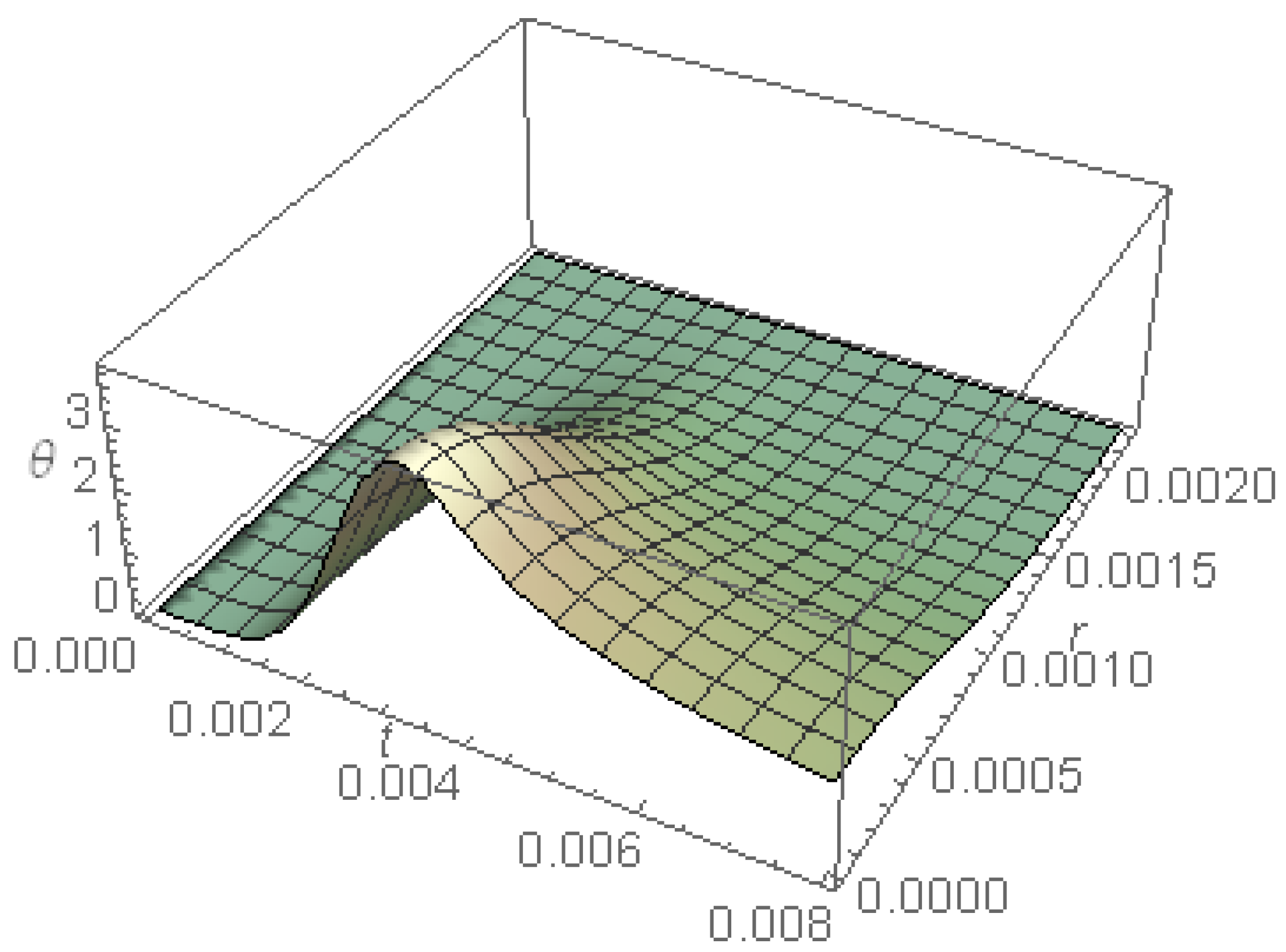
Figure 1 represents the surface temperature $\theta \left(r,0,t\right)$ calculated for ${\tau }_1=0.6 {\tau }_2$ in the absence of cooling. The figure shows that the surface temperature increases until it reaches its maximum, which clearly shifted to a greater time than that of the maximum of $Q(t)$$\left(3\times {10}^{-3}\right)$. After $\theta \left(r,0,t\right)$ reaches its maximum, it begins to decrease and does not reach the zero-value even after the pulse is switched off. Moreover, in the radial direction, $\theta \left(r,0,t\right)$ has a weak gradient near the surface; this gradient becomes stronger as r-increases until the temperature vanishes. The behavior of the temperature depends on two main occurrences, namely, the conductivity of the material and the absorbed energy, where at the beginning of the illumination process and due to the increased pulse, the absorbed energy will be greater than the conductivity of the material, so $\theta \left(r,0,t\right)$ increases; this behavior lasts up to when the absorbed energy is matched to the conducted energy; exactly at this time, the surface temperature attains its maximum. After that, and according to the chosen pulse shape, the absorbed energy begins to decrease, and the conductivity of the material gains the upper hand; this leads to a decrease in the surface temperature. After the pulse is switched off, the gradient of the temperature becomes smaller than that during the pulse, which is due to the absence of the laser radiation; this leads to a small gradient and, consequently, small conduction of the heat energy.

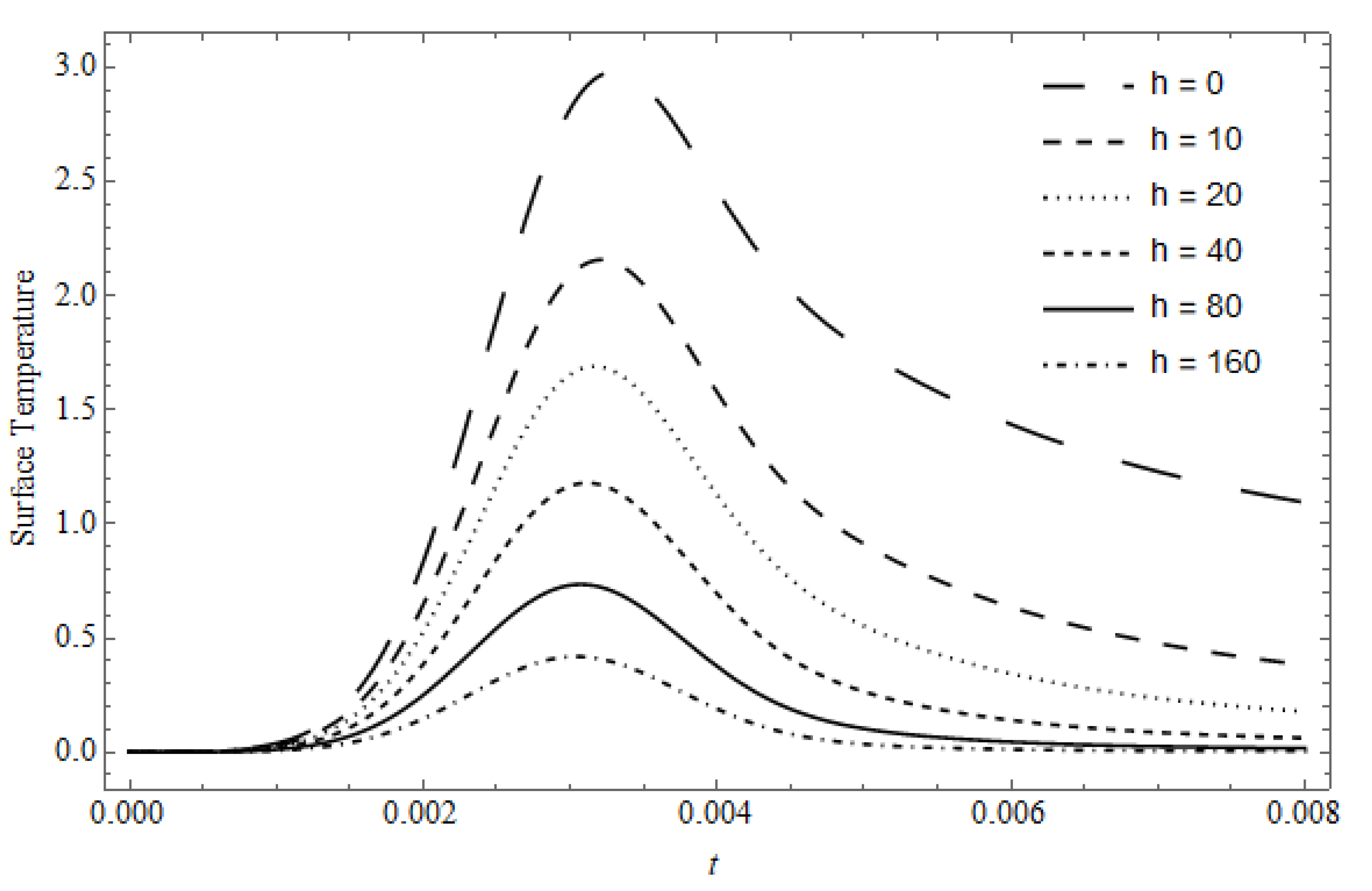
Figure 2 represents the time-dependent surface temperature, with $h$ as a parameter, calculated for ${\tau }_1= 0.6 {\tau }_2$ and $r=5\times {10}^{- 4}$. As expected, the surface temperature clearly decreases with increasing values of the cooling coefficient; moreover, as the cooling coefficient takes small values, the maximum value of the surface temperature is shifted towards greater time than that of the maximum of $Q\left(t\right).$ Beside the general decrease in surface temperature with increasing $h$, its behavior after it reaches its maximum, and at the times where the laser is switched off, decreases until the surface temperature approximately takes the shape of $Q\left(t\right).$ This behavior is due to the contribution of the cooling effect together with the conductivity of the material, especially after the laser is switched off and the absorbed energy is stopped.

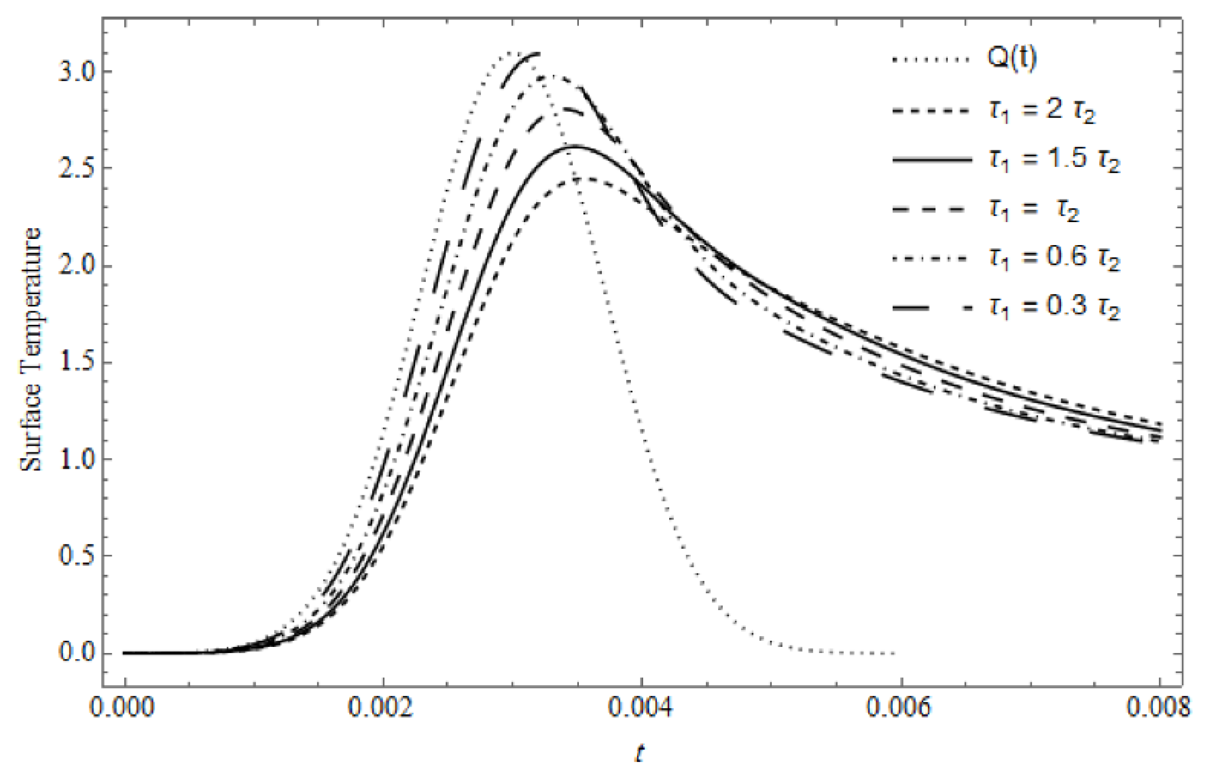
Figure 3 represents the time-dependent laser pulse shape and the surface temperature, with ${\tau }_1$ as a parameter in the absence of cooling, calculated for $r=5\times {10}^{- 4}$. The figure shows that compared to the chosen temporal pulse shape, $Q\left(t\right)$, for ${\tau }_1>{\tau }_2$, the maximum surface temperature becomes smaller and shifts evidently towards greater time than that for ${\tau }_1<{\tau }_2$. This means that the surface temperature for ${\tau }_1>{\tau }_2$ needs more time and consumes more energy to reach its maximum; this behavior is similar to the behavior that appears in [31] for the classical coupled theory.

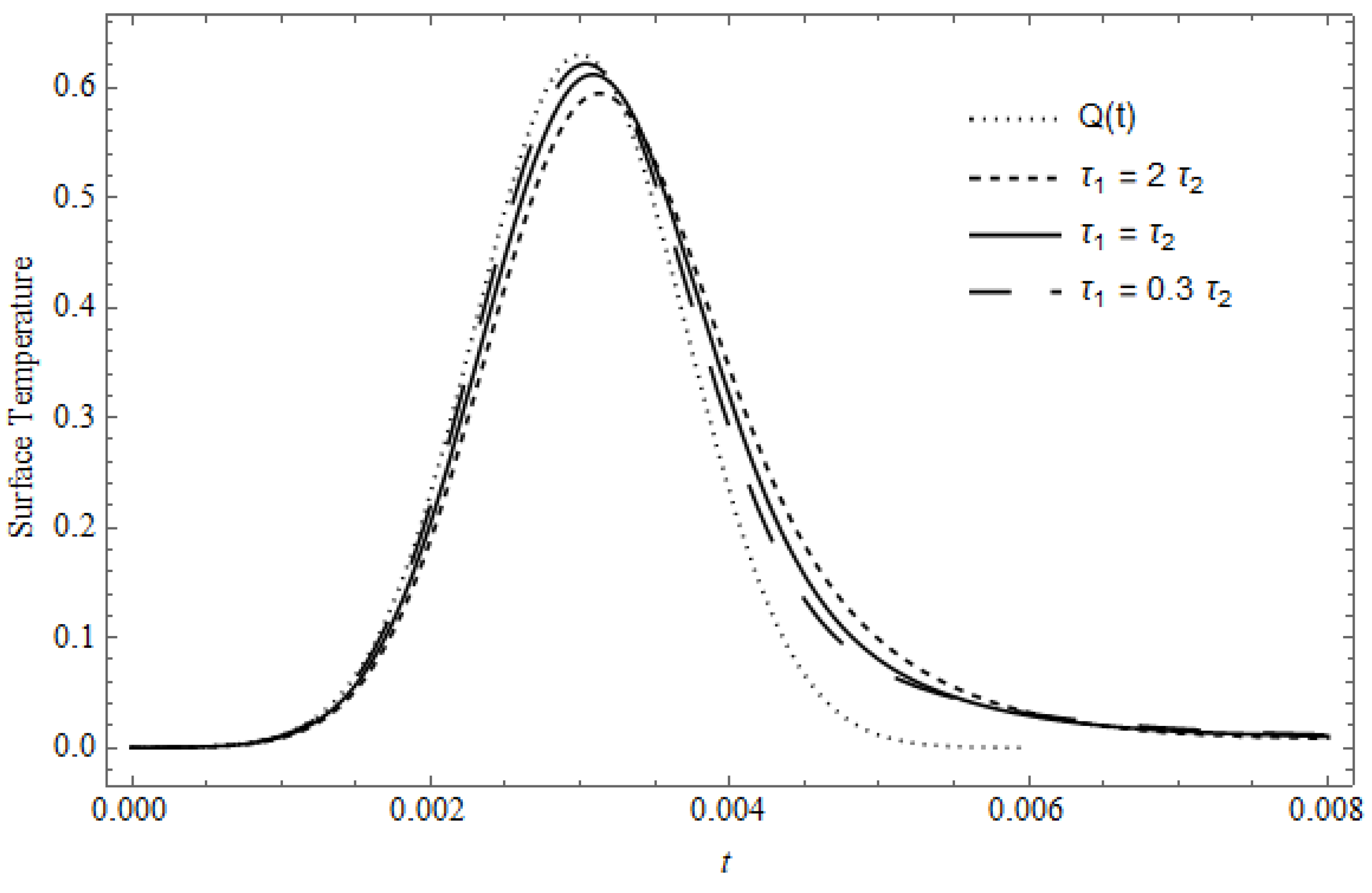
Figure 4 represents the time-dependent laser pulse shape and the surface temperature, with ${\tau }_1$ as a parameter in the presence of heat losses, calculated for $h=100$, $r=5\times {10}^{- 4}$, and $t=4\times {10}^{- 3}$. As seen, the effect of cooling is very pronounced, where the values of the surface temperature are decreased and its maximum is slightly shifted from the time of the maximum of $Q\left(t\right)$. Moreover, after the laser is switched off, the temperature approximately reaches zero, which does not occur in the absence of cooling; these behaviors are due to the cooling and the conductivity of the material. The behavior of this figure is slightly similar to the behavior of the previous figure, where the time needed to reach the peak is slightely shifted towards greater time for ${\tau }_1>{\tau }_2$ than for ${\tau }_1<{\tau }_2.$

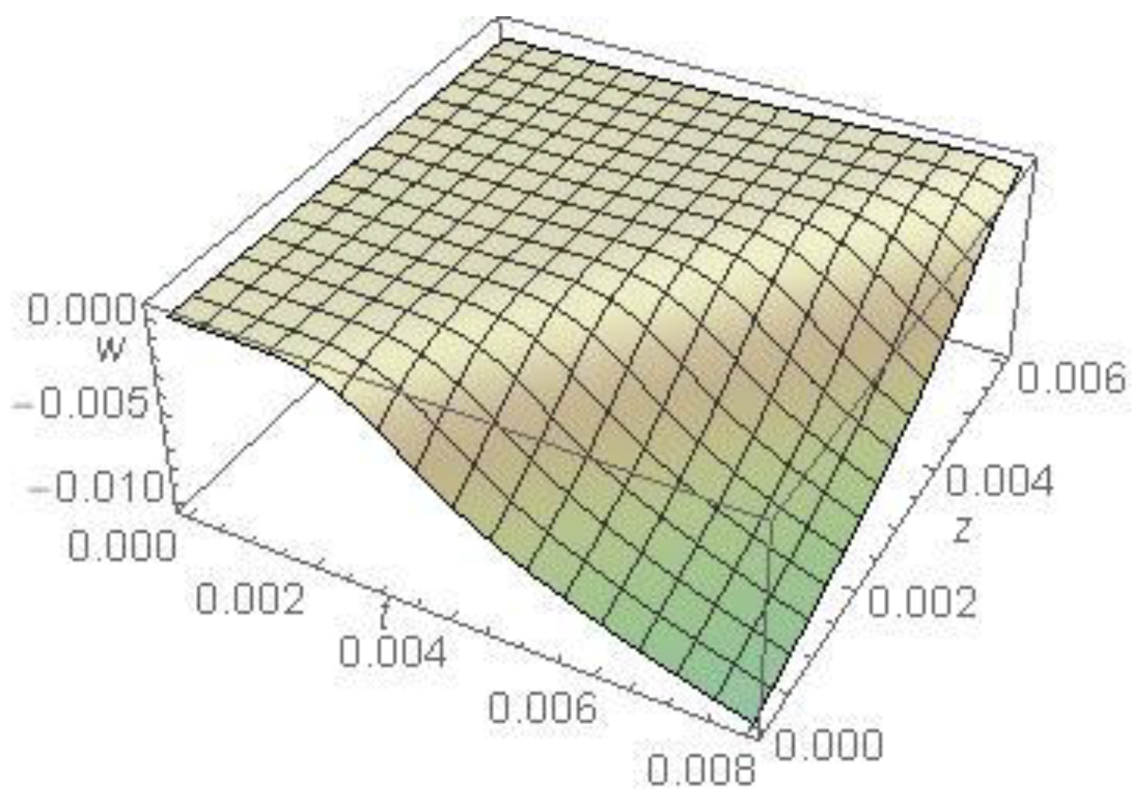
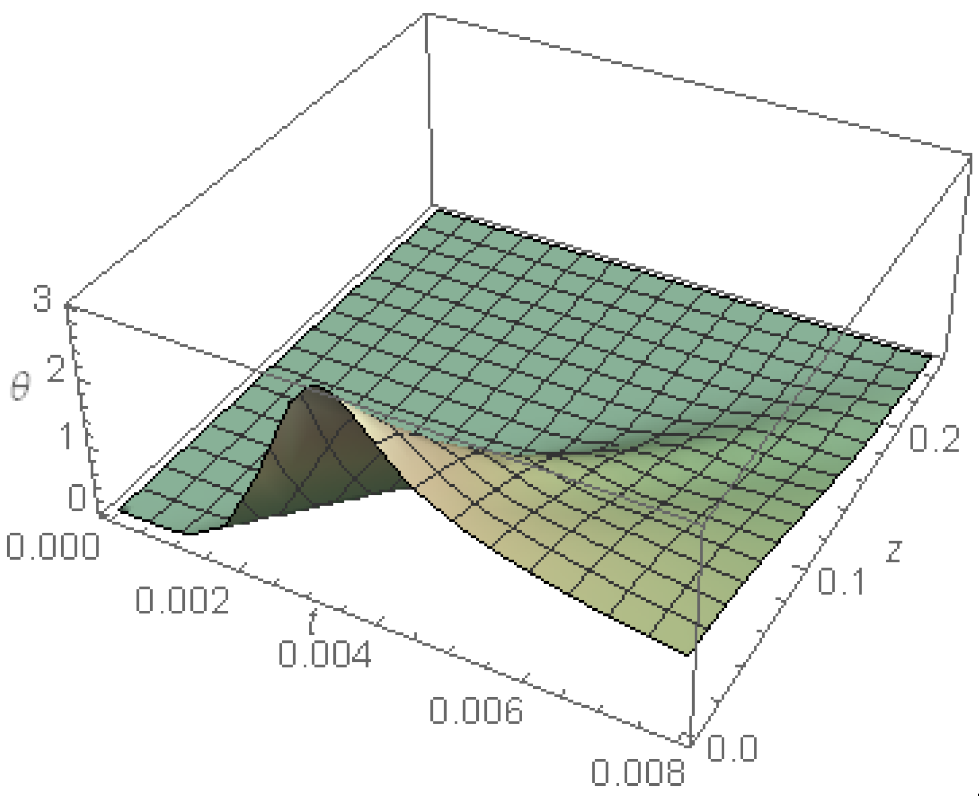
Figure 5 represents the temperature $\theta$ as a function of $z$ and $t$ in the absence of cooling, calculated for ${\tau }_1=0.6 {\tau }_2$ and $r=5\times {10}^{- 4}$. The finite velocity that distinguishes the DPL model appears evidently through the strong gradient at all locations, especially before the pulse is switched off. After the temperature reaches its maximum, a small temperature gradient begins to appear near the surface. The figure shows that the temperature is fully compatible with the time pulse profile, where the temperature increases until it reaches its maximum and then begins to decline. The temperature shows its highest value at the irradiated surface; this value decreases as z increases until it vanishes.

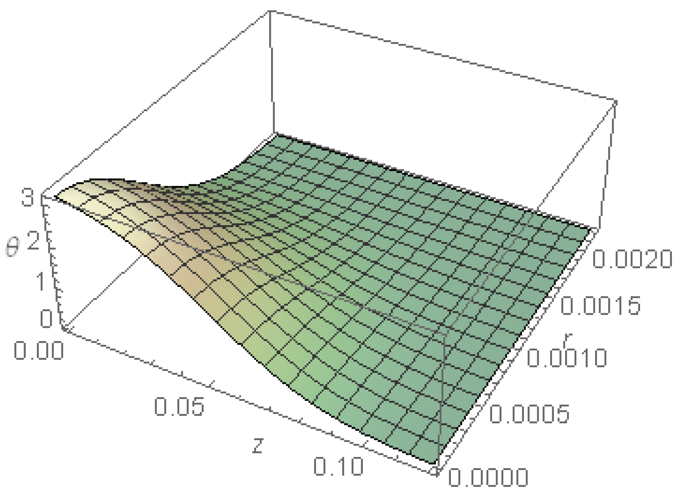
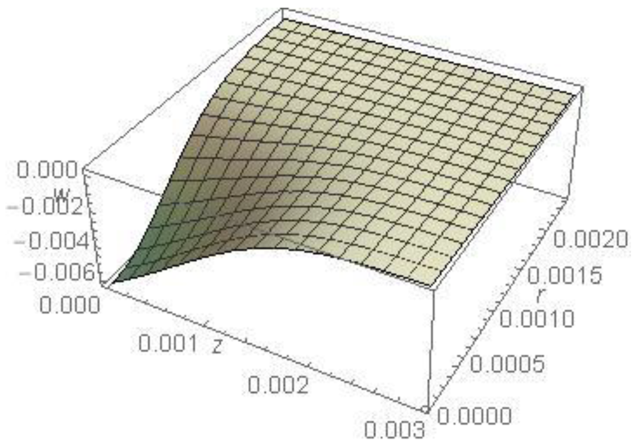
Figure 6 represents the temperature of the medium as a function of $z$ and $r$ in the absence of cooling, calculated for ${\tau }_1=0.6 {\tau }_2$ and $t=4\times {10}^{- 3}$. It is evident that the maximum temperature occurs at the illuminated surface and the temperature has a weak gradient in a small region adjacent to the target surface, as $z$ and $r$ increases; the gradient becomes strong until the temperature vanishes. This figure agrees with the previous figure, for which the finite velocity of the employed model evidently appears.

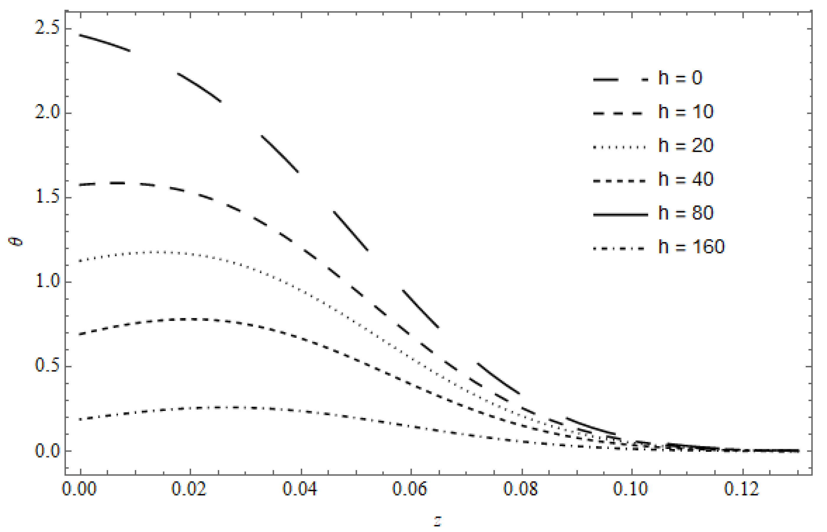
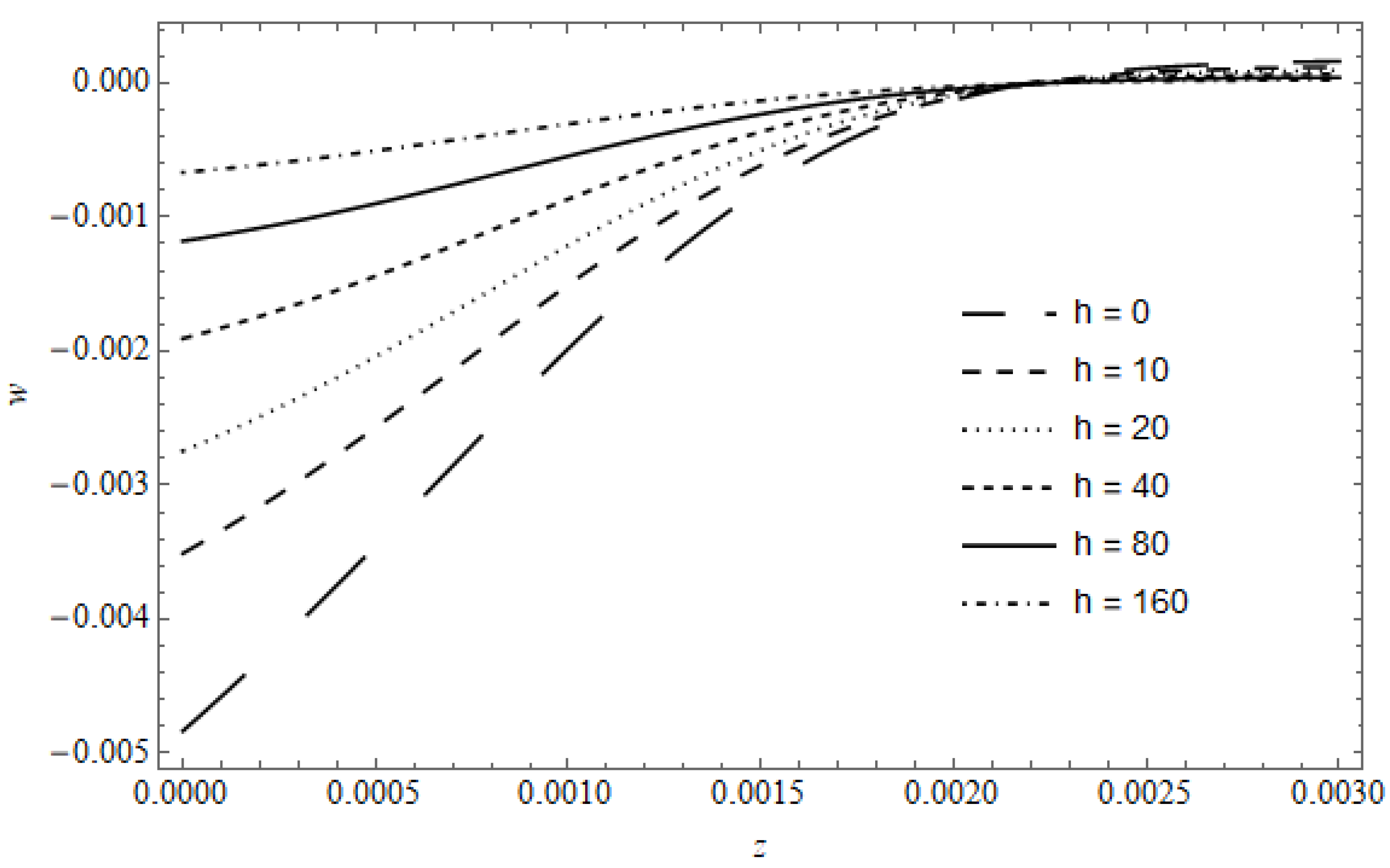
Figure 7 represents the temperature versus z, with $h$ as a parameter, calculated for ${\tau }_1= 0.6 {\tau }_2$ and $r=5\times {10}^{- 4}$. As expected, the temperature decreases as h increases; moreover, a weak gradient near the surface is observed; this gradient moves deeper into the medium as $h$ increases. The maximum temperature is slightly shifted, nearer to the surface; this behavior can be observed from the value $h=20.$

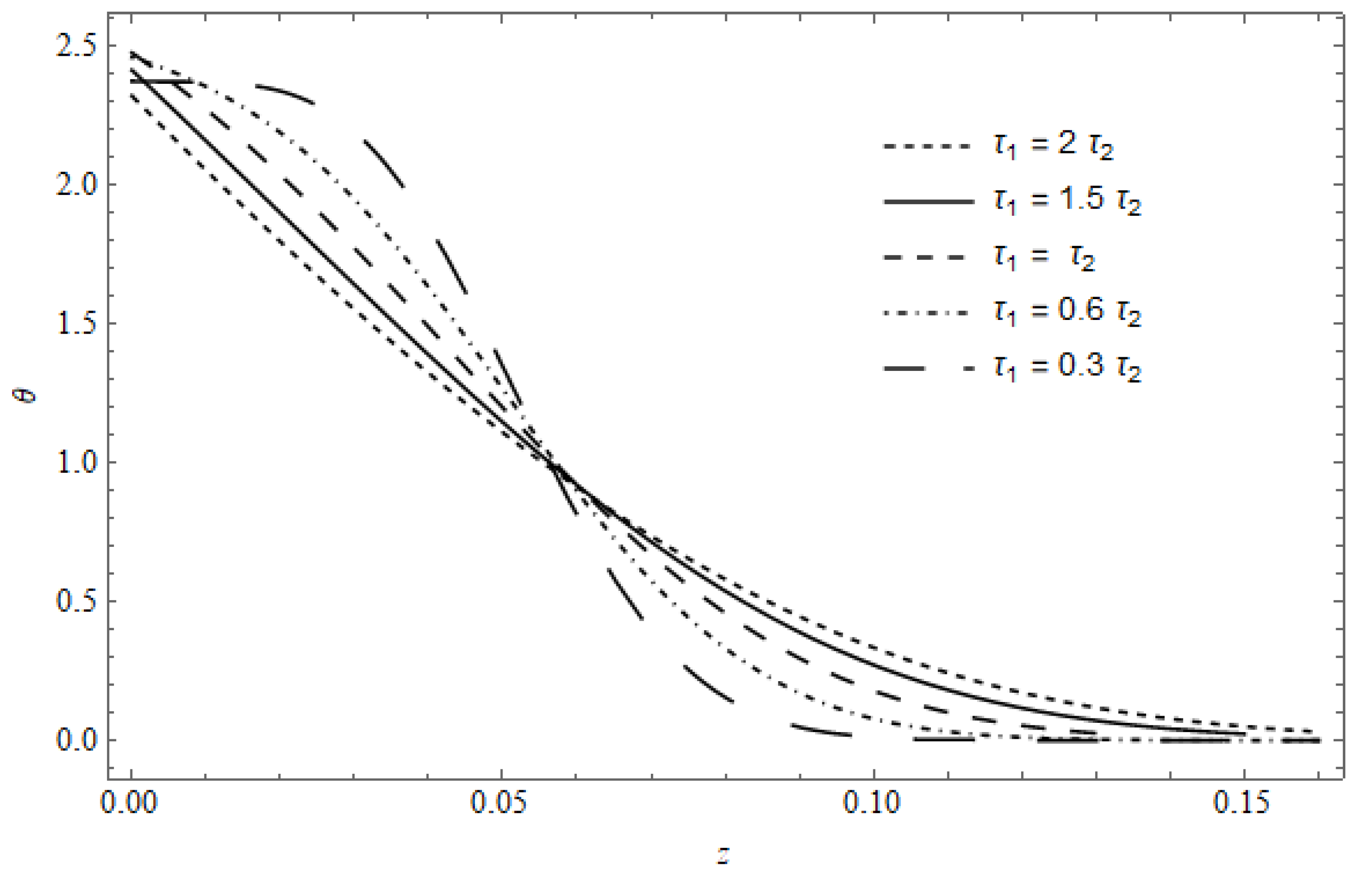
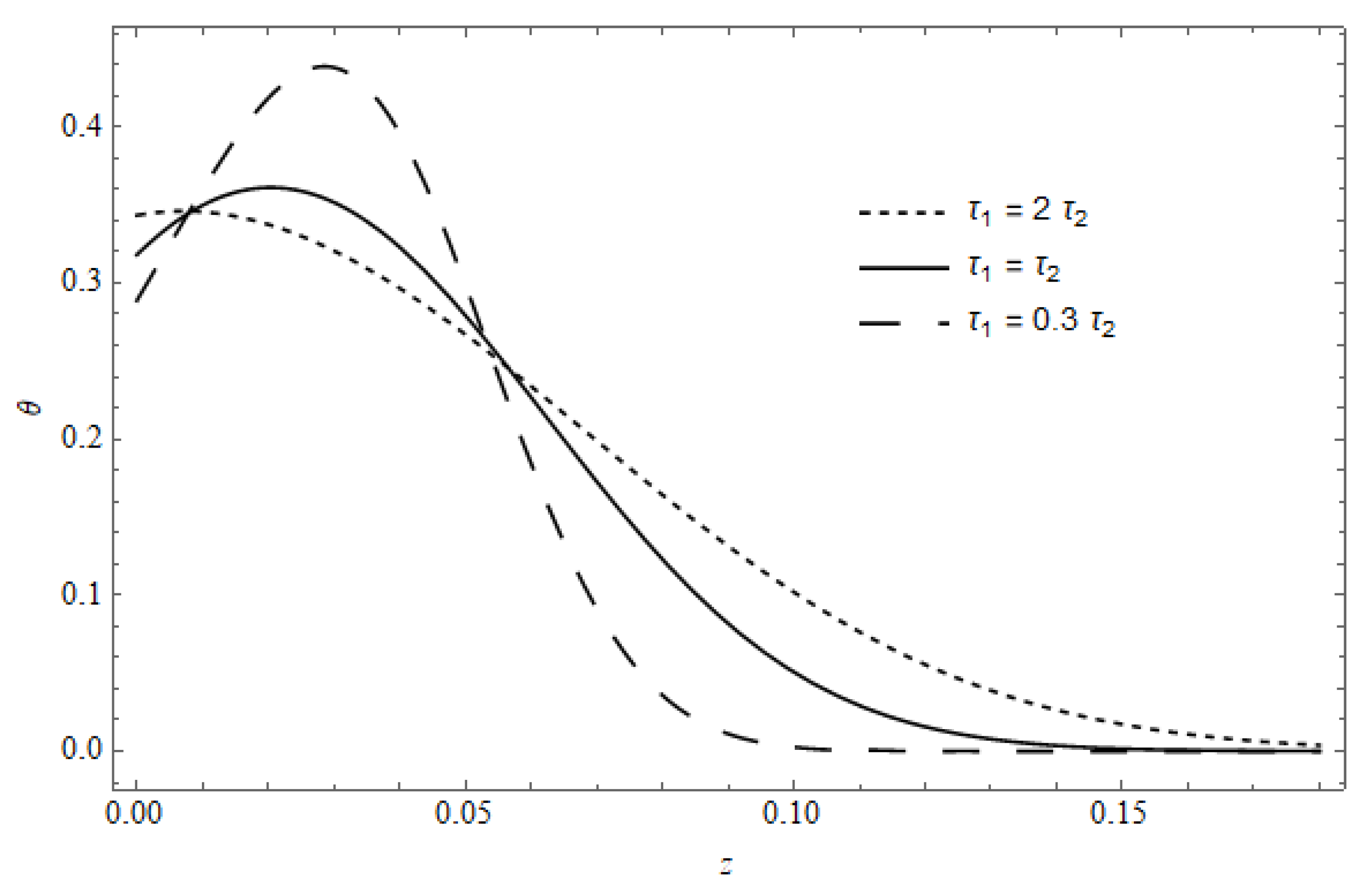
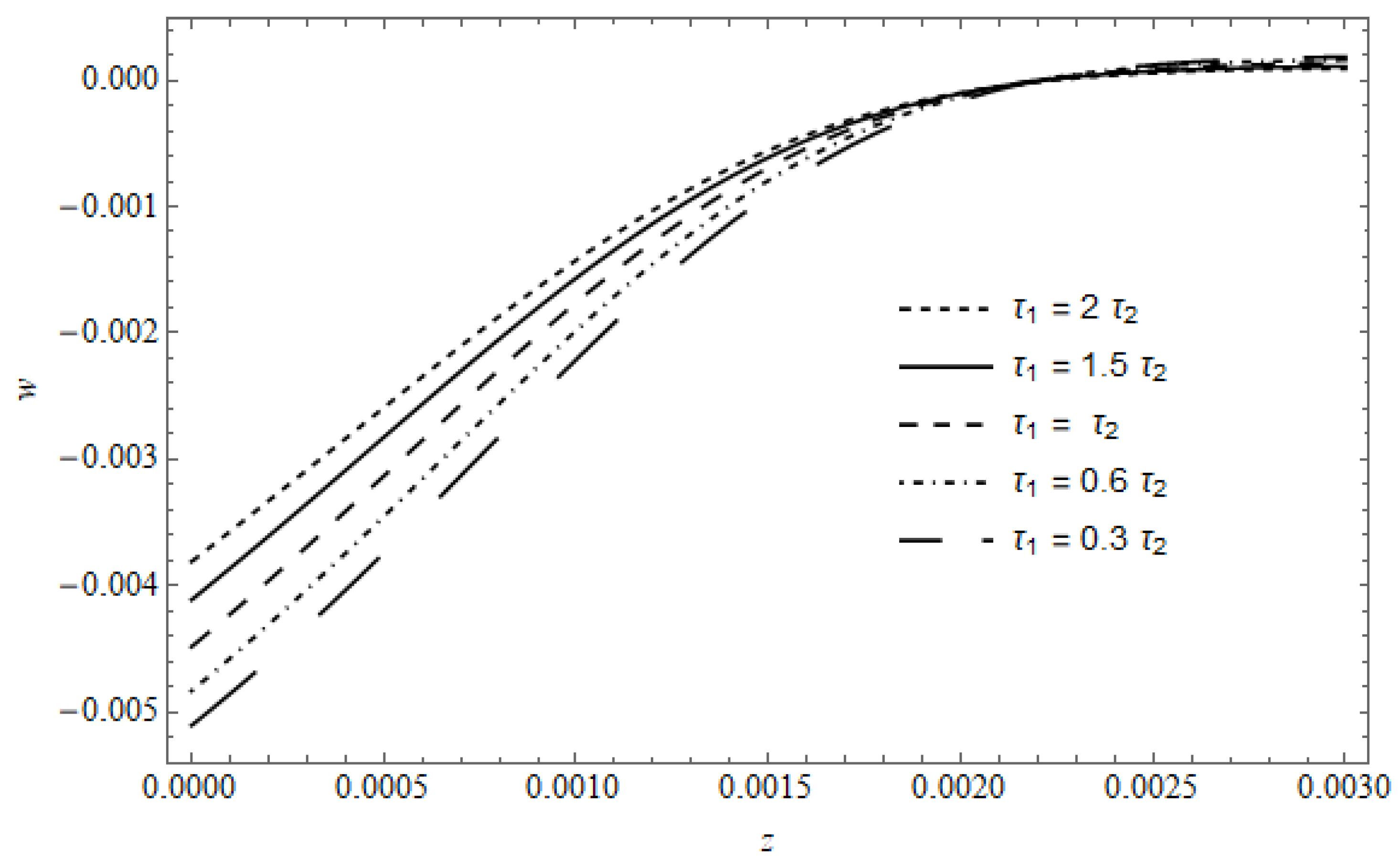
Figure 8 represents the temperature versus z in the absence of cooling, with ${\tau }_1$ as a parameter, calculated for $r=5\times {10}^{- 4}$ and $t=4\times {10}^{- 3}$. The figure shows that, near the surface, the temperature gradients in the case of ${\tau }_1>{\tau }_2$ are stronger than that of ${\tau }_1<{\tau }_2$, which has lower gradients; this behavior is evident for the curve of ${\tau }_1=0.3 {\tau }_2$. Additionally, the penetration of temperature into the medium increases as ${\tau }_1$ increases and becomes greater as ${\tau }_1>{\tau }_2$; this behavior is clearly shown for ${\tau }_1=2 {\tau }_2$, demonstrated by comparison with the other values of ${\tau }_1$. Again, the behavior of the temperature when ${\tau }_1>{\tau }_2$ is similar to the behavior of the classical coupled theory of thermoelasticity in [31].

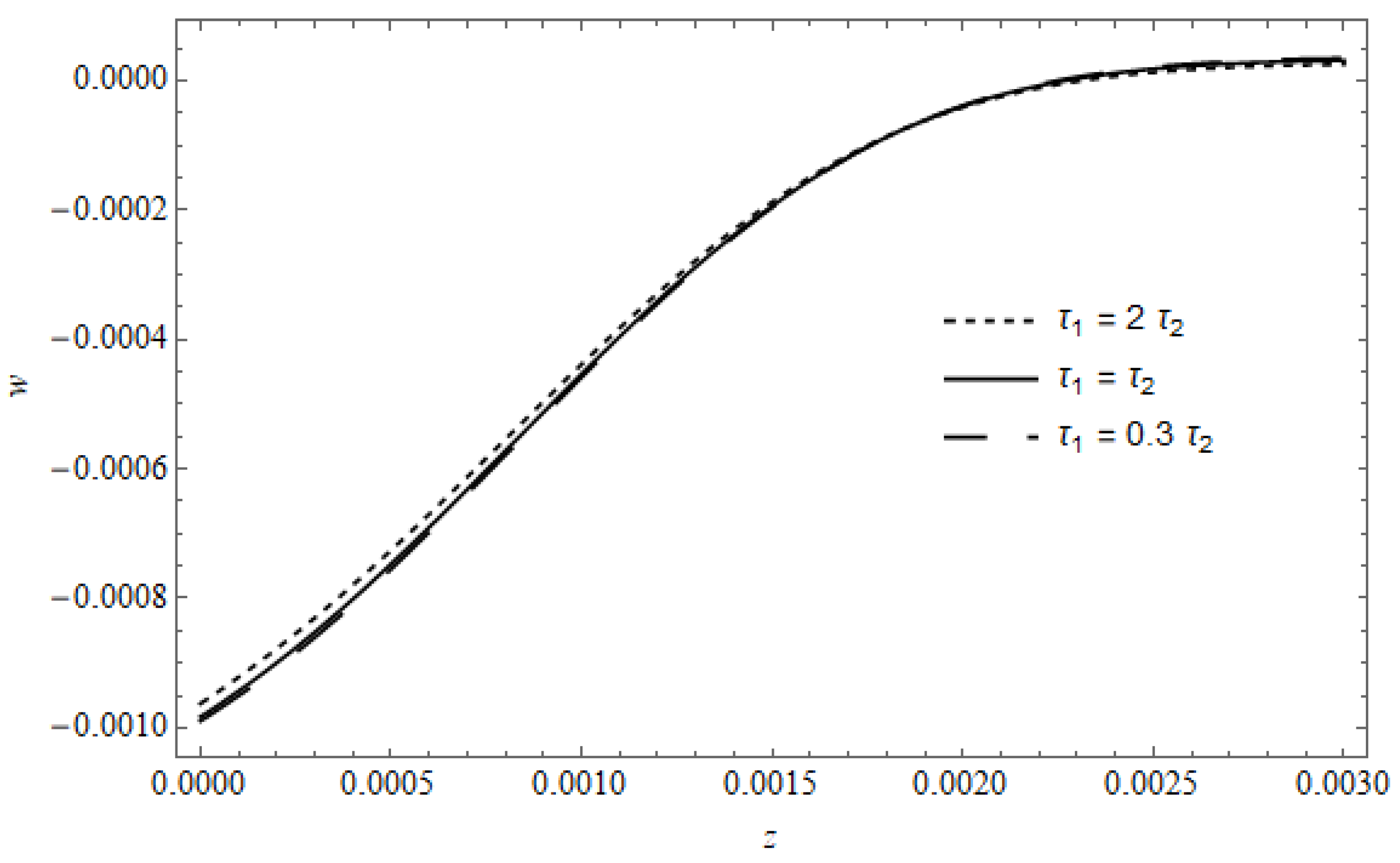
Figure 9 represents the temperature distribution versus z, with ${\tau }_1$ as a parameter, calculated for $h=100$, $r=5\times {10}^{- 4}$ and $t=4\times {10}^{- 3}$. The main behavior of the previous figure is observed here for both the gradient of the temperature and the penetration into the medium. The figure shows a pronounced contribution to the cooling, where for ${\tau }_1\le {\tau }_2$ it is clear that the maximum does not occur at the illuminated surface but is shifted to greater $z$ values and the temperature at the surface decreases as ${\tau }_1$ decreases.

Figure 10 represents the component of the displacement $w$ of the medium as a function of $z$ and $t$ in the absence of cooling, calculated for ${\tau }_1=0.6{\tau }_2$ and $r=5\times {10}^{- 4}.$ The negative sign of the displacement refers to its direction, where it occurs in the direction of the free surface. As seen, the displacement does not show a behavior before the time $t=0.002$; this behavior is attributed to the small temperature at this time; moreover, the displacement increases with increased time. The maximum displacement appears at the surface and decreases as $z$ takes greater values until it vanishes; this behavior is due to temperature behavior.

Figure 11 represents the component of the displacement $w$ of the medium as a function of $z$ and $r$ in the absence of cooling, calculated for ${\tau }_1=0.6{\tau }_2$ and $t=4\times {10}^{- 3}.$ This figure agrees with the previous figure, where the maximum displacement is observed at the surface and decreases by increasing both $z$ and $r$. The figure also shows a negative sign for the displacement in the r-direction; this behavior is due to a decrease in the distance between the particles in the r-direction.

Figure 12 represents the distribution of the displacement $w$, with $h$ as a parameter, calculated for ${\tau }_1= 0.6 {\tau }_2$ and $r=5\times {10}^{- 4}$. As seen from the figure, the displacement decreases with an increase in $h$; this behavior is owed to the decrease in the corresponding temperature (see Figure 7).

Figure 13 represents the displacement $w$ in the absence of cooling, with ${\tau }_1$ as a parameter, calculated for $r=5\times {10}^{- 4}$ and $t=4\times {10}^{- 3}$. The figure shows that as ${\tau }_1$ takes values greater than ${\tau }_2$, the displacement decreases, and vice versa. Observing the behaviors of both the temperature and the displacement, one can note that the smallest and deeper temperatures produce the smallest displacements; this conduct can be explained from Figure 8, where for ${\tau }_1>{\tau }_2$, the gradient of the temperature in the vicinity of the surface and the penetration into the medium is greater than in the case of ${\tau }_1<{\tau }_2$; this means that the first case consumes more energy in heating the surrounding and to penetrate than the second case and, thus, its temperature and displacement is the smallest.

Figure 14 represents the displacement $w$ with the existence of cooling, with ${\tau }_1$ as a parameter, calculated for $r=5\times {10}^{- 4}$ and $t=4\times {10}^{- 3}$. The figure shows a clear influence for the heat losses, where the difference between the three curves becomes approximately slight; this is despite the compatibility of the behavior of this figure with the previous figure.

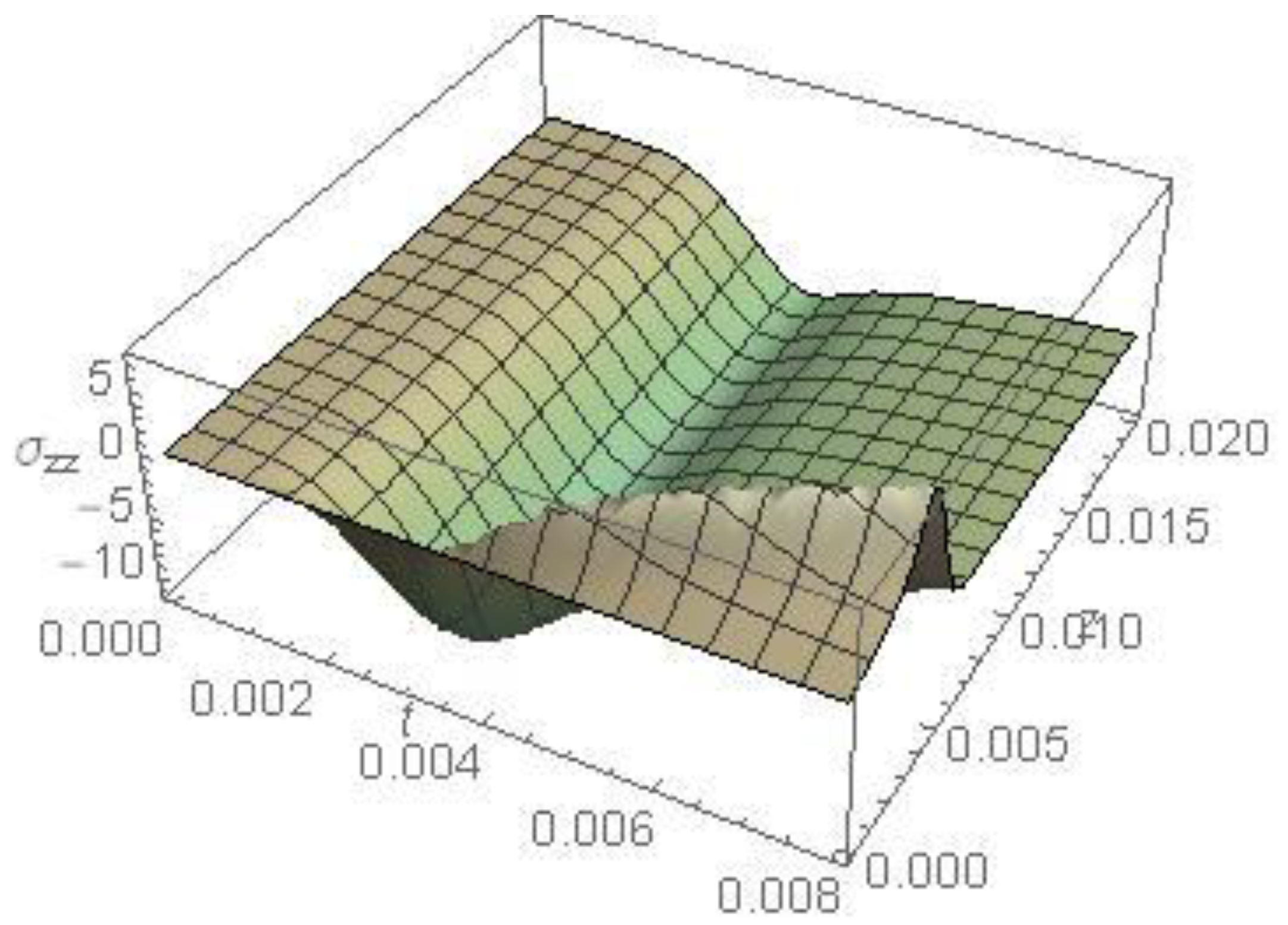
Figure 15 represents the stress component ${\sigma }_{zz}$ as a function of $z$ and $t$ in the absence of cooling, calculated for ${\tau }_1=0.6 {\tau }_2$ and $r=5\times {10}^{- 4}$. The general behavior of ${\sigma }_{zz}$ depends on the behavior of both the gradient of the displacement and the temperature (see equation 7); hence, as seen, before the laser pulse reaches its peak, the temperature and the displacement increase, but the temperature has the superiority; this explains the negative values of ${\sigma }_{zz}$. After the laser pulse reaches its peak, the absorbed energy decreases, and then the temperature decreases while the displacement and its gradient are still increasing; this explains the positive values of ${\sigma }_{zz}$ near the surface. One can observe that this behavior is clear after the temperature reaches its maximum. By increasing z-values, the influence of the gradient of the displacement begins to decay to permit the temperature to gain the upper hand again; this gives ${\sigma }_{zz}$ negative values until the stress vanishes.

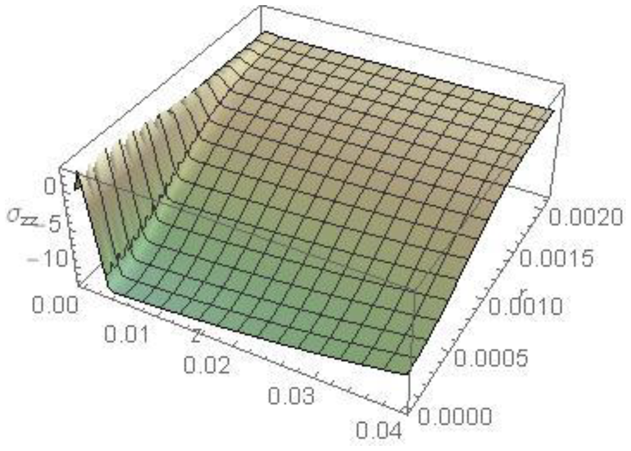
Figure 16 represents the stress component ${\sigma }_{zz}$ as a function of $z$ and $r$ in the absence of cooling, calculated for ${\tau }_1=0.6 {\tau }_2$ and $t=4\times {10}^{- 3}$. It is clear that the stress ${\sigma }_{zz}$ at the surface satisfies the boundary condition for all values of r. Near the surface, ${\sigma }_{zz}$ begins to increase until it reaches a maximum value, then it decreases with increasing $z$ until the stress vanishes (this will be seen in a later figure). The figure also shows that except at the surface $\left(z=0\right)$, the stress begins with a maximum value in the r-direction, then decreases until it vanishes.

Figure 17 represents the stress component ${\sigma }_{zz}$ versus z, with $h$ as a parameter, calculated for ${\tau }_1= 0.6 {\tau }_2$ and $r=5\times {10}^{- 4}$. As seen for different $h$ values, the stresses in the vicinity of the surface are almost identical in their gradients. As z increases, the performance of the temperature with cooling appears evident, as in Figure 7.

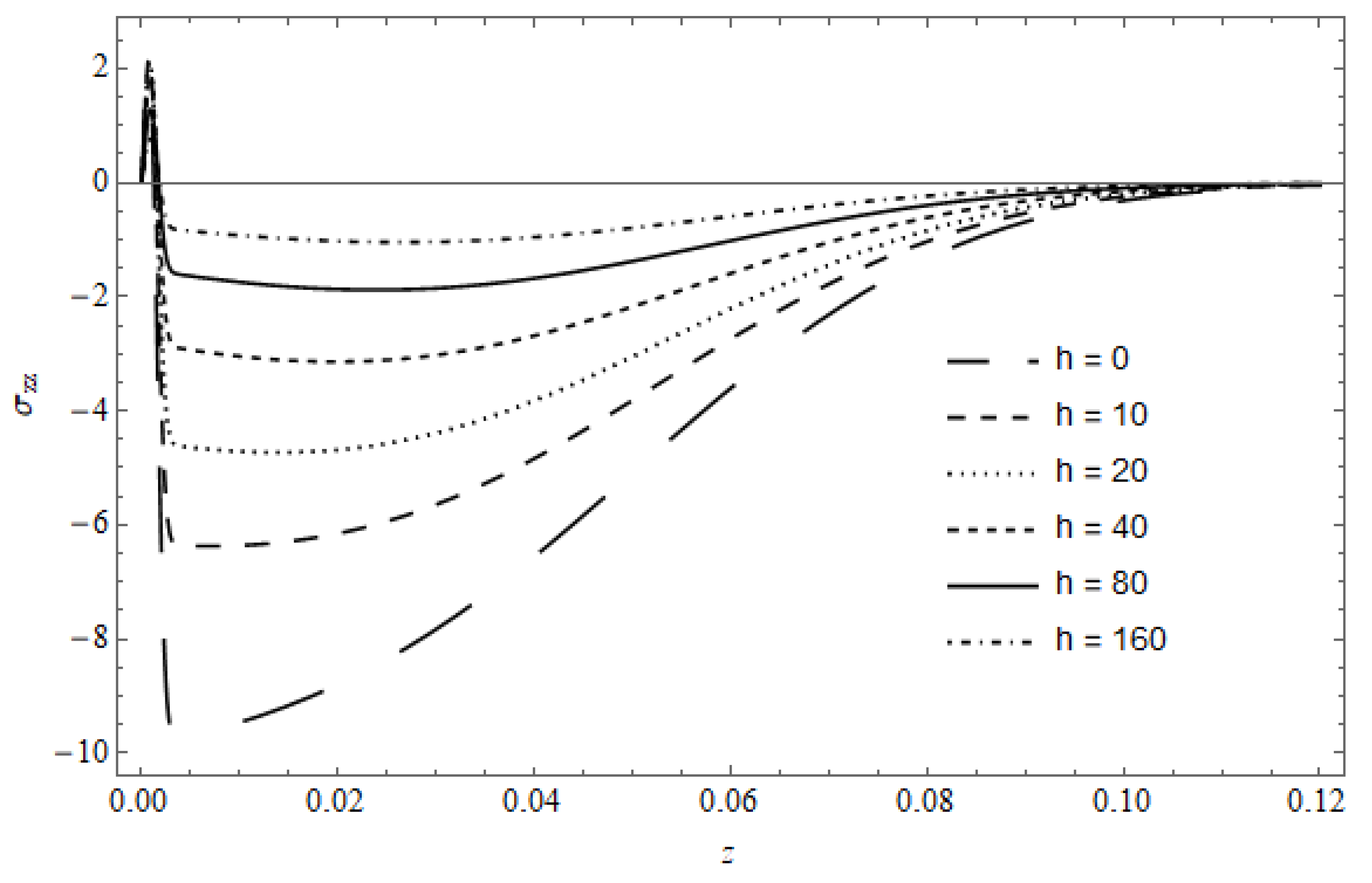
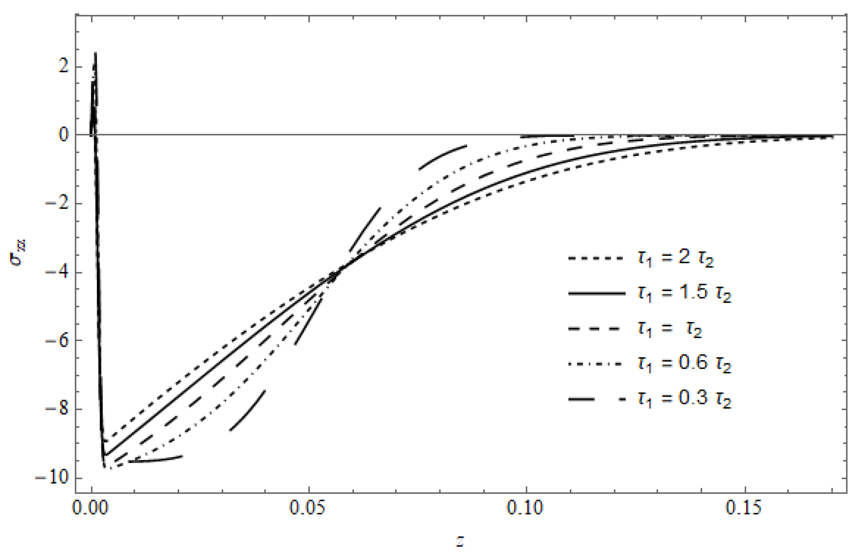
Figure 18 represents the stress component ${\sigma }_{zz}$ versus z in the absence of cooling, with ${\tau }_1$ as a parameter, calculated for $r=5\times {10}^{- 4}$ and $t=4\times {10}^{- 3}$. The figure shows that the stress in the vicinity of the surface is slightly affected by ${\tau }_1$; as z increases, a pronounced effect for ${\tau }_1$ is observed, where the behavior of the temperature appears with ${\tau }_1$ (see Figure 8).

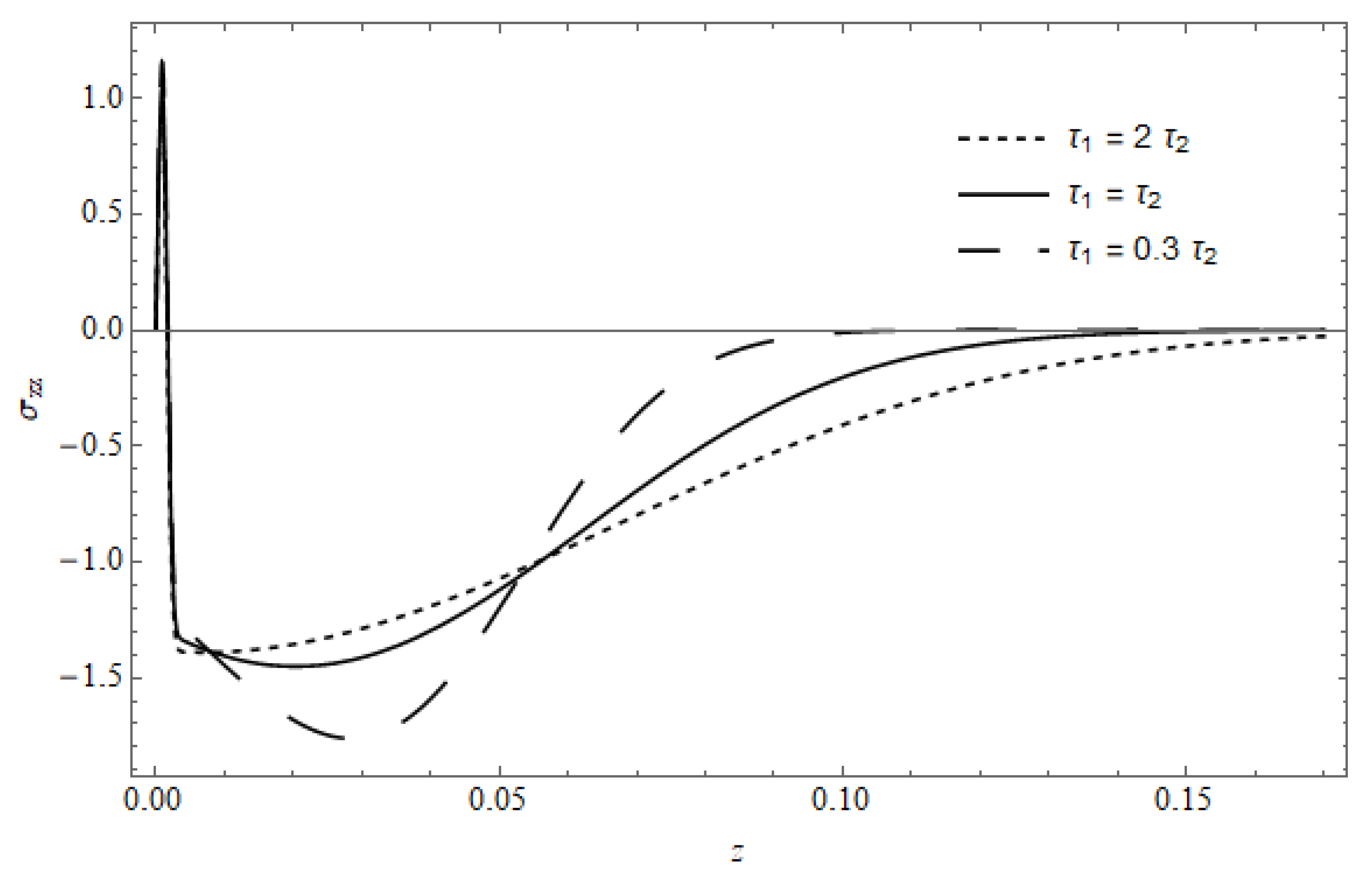
Figure 19 represents the stress component ${\sigma }_{zz}$ versus z, with ${\tau }_1$ as a parameter in the existence of cooling, calculated for $r=5\times {10}^{- 4}$ and $t=4\times {10}^{- 3}$. As seen, the behavior of ${\sigma }_{zz}$ at the surface coincides for the three curves; as z increases, the effect of the temperature is clear (see Figure 9).

8. Conclusions

In this paper, the response generated by the volumetric absorption technique of laser pulse in a 2D generalized thermoelastic semi-infinite medium is discussed in the absence and presence of temperature-dependent heat losses by employing the DPL model. From the above discussion, it can be deduced that

• The results obtained in the absence and presence of cooling are not in conflict with well-known physical conduct, especially for ${\tau }_1<{\tau }_2$.
• The translation times show clear effects on the behavior of all the studied fields in the absence of cooling and on some studied fields in the presence of cooling.
• For ${\tau }_1>{\tau }_2$, the thermoelastic response of the DPL model behaves similar to the thermoelastic response of the classical coupled theory of thermoelasticity.
• The heat losses show a pronounced effect, especially on the temperature, in which its maximum shifted into the medium.

References

1. Biot, M.A. Thermoelasticity and Irreversible Thermodynamics. J. Appl. Phys. 1956, 27, 240–253. [Google Scholar] [CrossRef]
2. Al-Huniti, N.S.; Al-Nimr, M. Thermoelastic response of a heated thin composite plate using the hyperbolic heat conduction model: Lumped analysis. Int. J. Therm. Sci. 2004, 43, 959–965. [Google Scholar] [CrossRef]
3. Povstenko, Y. Fractional Thermoelasticity; Springer: New York, NY, USA, 2015. [Google Scholar]
4. Lord, H.; Shulman, Y. A generalized dynamical theory of thermoelasticity. J. Mech. Phys. Solids 1967, 15, 299–309. [Google Scholar] [CrossRef]
5. Cattaneo, C. Sulla Conduzione Del Calore. Some Asp. Diffus. Theory 1948, 3, 83–101. [Google Scholar]
6. Cattaneo, C. A form of heat conduction equation which eliminates the paradox of instantaneous propagation. C. R. Chim. 1958, 247, 431–433. [Google Scholar]
7. Green, A.E.; Lindsay, K.A. Thermoelasticity. J. Elast. 1972, 2, 1–7. [Google Scholar] [CrossRef]
8. Green, A.E.; Naghdi, P.M. Thermoelasticity without energy dissipation. J. Elast. 1993, 31, 189–208. [Google Scholar] [CrossRef]
9. Hetnarski, R.B.; Ignaczak, J. Soliton-like waves in a low temperature nonlinear thermoelastic solid. Int. J. Eng. Sci. 1996, 34, 1767–1787. [Google Scholar] [CrossRef]
10. Tzou, D.Y. A Unified Field Approach for Heat Conduction from Macro- to Micro-Scales. J. Heat Transf. 1995, 117, 8–16. [Google Scholar] [CrossRef]
11. Tzou, D.Y. The generalized lagging response in small-scale and high-rate heating. Int. J. Heat Mass Transf. 1995, 38, 3231–3240. [Google Scholar] [CrossRef]
12. Zenkour, A.M.; Mashat, D.; Abouelregal, A. The effect of dual-phase-lag model on reflection of thermoelastic waves in a solid half space with variable material properties. Acta Mech. Solida Sin. 2013, 26, 659–670. [Google Scholar] [CrossRef]
13. Othman, M.I.A.; Abd-Elaziz, E.M. The Effect of Thermal Loading Due to Laser Pulse in Generalized Thermoelastic Medium with Voids in Dual Phase Lag Model. J. Therm. Stress. 2015, 38, 1068–1082. [Google Scholar] [CrossRef]
14. Lotfy, K. The elastic wave motions for a photothermal medium of a dual-phase-lag model with an internal heat source and gravitational field. Can. J. Phys. 2016, 94, 400–409. [Google Scholar] [CrossRef] [Green Version]
15. Abbas, I.A.; Mohamed, E.A.E. Dual-Phase-Lag Model on Generalized Magneto-Thermoelastic Interaction in a Functionally Graded Material. Int. J. Acoust. Vib. 2017, 22, 369–376. [Google Scholar] [CrossRef]
16. Abouelregal, A.; Abo-Dahab, S.M. A two-dimensional problem of a mode-I crack in a rotating fibre-reinforced isotropic thermoelastic medium under dual-phase-lag model. Sadhana 2018, 43, 13. [Google Scholar] [CrossRef] [Green Version]
17. Kalkal, K.K.; Sheokand, S.K.; Deswal, S. Reflection and transmission between thermoelastic and initially stressed fiber-reinforced thermoelastic half-spaces under dual-phase-lag model. Acta Mech. 2019, 230, 87–104. [Google Scholar] [CrossRef]
18. Othman, M.I.A.; Abd-Elaziz, E.M.; Hilal, M.I.M. State-space approach to a 2-D generalized thermoelastic medium under the effect of inclined load and gravity using a dual-phase-lag model. Mech. Based Des. Struct. Mach. 2020, 1–17. [Google Scholar] [CrossRef]
19. Allam, M.N.; Tayel, I.M. Thermal effect on transverse vibrations of a nonhomogeneous rectangular thin plate subjected to a known temperature distribution. Trans. Can. Soc. Mech. Eng. 2020, 44, 452–460. [Google Scholar] [CrossRef]
20. Hassan, A.; El-Nicklawy, M.; El-Adawi, M.; Nasr, E.; Hemida, A.; El-Ghaffar, O. Heating effects induced by a pulsed laser in a semi-infinite target in view of the theory of linear systems. Opt. Laser Technol. 1996, 28, 337–343. [Google Scholar] [CrossRef]
21. Ezzat, M.A.; El Karamany, A.S.; Fayik, M.A. Fractional Ultrafast Laser–Induced Thermo-Elastic Behavior in Metal Films. J. Therm. Stress. 2012, 35, 637–651. [Google Scholar] [CrossRef]
22. Henain, E.F.; Hassan, A.F.; Megahed, F.; Tayel, I.M. Thermo-Elastic Half Space Under Illumination of a Laser Beam by Using Lord and Shulman Theory. J. Therm. Stress. 2014, 37, 51–72. [Google Scholar] [CrossRef]
23. Youssef, H.M.; El-Bary, A.A. Thermoelastic Material Response Due to Laser Pulse Heating in Context of Four Theorems of Thermoelasticity. J. Therm. Stress. 2014, 37, 1379–1389. [Google Scholar] [CrossRef]
24. Elhagary, M.A. A Two-Dimensional Generalized Thermoelastic Diffusion Problem for a Thick Plate Subjected to Thermal Loading Due to Laser Pulse. J. Therm. Stress. 2014, 37, 1416–1432. [Google Scholar] [CrossRef]
25. Zenkour, A.M.; Aboelregal, A.E. The fractional effects of a two-temperature generalized thermoelastic semi-infinite solid induced by pulsed laser heating. Arch. Mech. 2015, 67, 53–73. [Google Scholar]
26. Bassiouny, E.; Abouelnaga, Z.; Youssef, H.M. One-dimensional thermoelastic problem of a laser pulse under fractional order equation of motion. Can. J. Phys. 2017, 95, 464–471. [Google Scholar] [CrossRef]
27. Allam, M.N.M.; Tayel, I.M. Generalized thermoelastic functionally graded half space under surface absorption of a laser radiation. J. Theor. Appl. Mech. 2017, 55, 155–165. [Google Scholar] [CrossRef]
28. Abbas, I.A.; Marin, M. Analytical solution of thermoelastic interaction in a half-space by pulsed laser heating. Physica E Low Dimens. Syst. Nanostruct. 2017, 87, 254–260. [Google Scholar] [CrossRef]
29. Abouelregal, A.E.; Zenkour, A.M. A generalized thermoelastic medium subjected to pulsed laser heating via a two-temperature model. J. Theor. Appl. Mech. 2019, 57, 631–639. [Google Scholar] [CrossRef]
30. Tayel, I.M.; Hassan, A.F. Heating a thermoelastic half space with a surface absorption pulsed laser using fractional order theory of thermoelasticity. J. Theor. Appl. Mech. 2019, 57, 489–500. [Google Scholar] [CrossRef]
31. Tayel, I.M. Thermoelastic Response Induced by Volumetric Absorption of Uniform Laser Radiation in a Half-Space. Coatings 2020, 10, 228. [Google Scholar] [CrossRef] [Green Version]
32. Hetnarski, R. Coupled One-Dimensional Thermal Shock Problem for Small Times. Arch. Mech. 1961, 13, 295–306. [Google Scholar]
33. Hetnarski, R. The Fundamental Solution of the Coupled Thermoelastic Problem for Small Times. Arch. Mech. 1964, 1, 16. [Google Scholar]
34. Sherief, H.H.; Darwish, A.A. A short time solution for a problem in thermoelasticity of an infinite medium with a spherical cavity. J. Therm. Stress. 1998, 21, 811–828. [Google Scholar] [CrossRef]
35. Sherief, H.H.; Elmisiery, A.E.M.; Elhagary, M.A. Generalized thermoelastic problem for an infinitely long hollow cylinder for short times. J. Therm. Stress. 2004, 27, 885–902. [Google Scholar] [CrossRef]
36. Sherief, H.H.; Hamza, F.A.; El-Latief, A.M.A. Wave propagation study for axi-symmetric 2D problems of a generalized thermo-visco-elastic half space. J. Therm. Stress. 2019, 42, 835–848. [Google Scholar] [CrossRef]
37. Debnath, L.; Bhatta, D. Integral Transforms and Their Applications; Taylor and Francis: New York, NY, USA, 2015. [Google Scholar]
38. Boley, B.A. Discontinuities in integral-transform solutions. Q. Appl. Math. 1962, 19, 273–284. [Google Scholar] [CrossRef] [Green Version]
39. Boley, B.A.; Hetnarski, R.B. Propagation of Discontinuities in Coupled Thermoelastic Problems. J. Appl. Mech. 1968, 35, 489–494. [Google Scholar] [CrossRef]
40. Tzou, D.Y. Experimental support for the lagging behavior in heat propagation. J. Thermophys. Heat Transf. 1995, 9, 686–693. [Google Scholar] [CrossRef]
Figure 1. The surface temperature θ ( r , 0 , t ) in the absence of cooling.
Mathematics 08 02094 g001
Figure 2. The time-dependent surface temperature vs. t with h as a parameter.
Mathematics 08 02094 g002
Figure 3. The time-dependent surface temperature vs. t with τ 1 as a parameter for h = 0 .
Mathematics 08 02094 g003
Figure 4. The time-dependent surface temperature vs. t with τ 1 as a parameter for h = 0 .
Mathematics 08 02094 g004
Figure 5. The temperature θ as a function of z and t in the absence of cooling.
Mathematics 08 02094 g005
Figure 6. The temperature θ as a function of z and r in the absence of cooling.
Mathematics 08 02094 g006
Figure 7. The temperature θ versus z , with h as a parameter for τ 1 = 0.6   τ 2 .
Mathematics 08 02094 g007
Figure 8. The temperature θ versus z , with τ 1 as a parameter in the absence of cooling.
Mathematics 08 02094 g008
Figure 9. The temperature θ versus z , with τ 1 as a parameter for h 0 .
Mathematics 08 02094 g009
Figure 10. The displacement w as a function of z and t in the absence of cooling.
Mathematics 08 02094 g010
Figure 11. The displacement w as a function of z and r in the absence of cooling.
Mathematics 08 02094 g011
Figure 12. The displacement w versus z , with h as a parameter for τ 1 = 0.6 τ 2 .
Mathematics 08 02094 g012
Figure 13. The displacement w versus z , with τ 1 as a parameter in the absence of cooling.
Mathematics 08 02094 g013
Figure 14. The displacement w versus z , with τ 1 as a parameter in the presence of cooling.
Mathematics 08 02094 g014
Figure 15. The stress σ z z as a function of z and t in the absence of cooling.
Mathematics 08 02094 g015
Figure 16. The stress σ z z as a function of z and r in the absence of cooling.
Mathematics 08 02094 g016
Figure 17. The stress σ z z versus z , with h as a parameter for τ 1 = 0.6 τ 2 .
Mathematics 08 02094 g017
Figure 18. The stress σ z z versus z with τ 1 as a parameter in the absence of cooling.
Mathematics 08 02094 g018
Figure 19. The stress σ z z versus z , with τ 1 as a parameter in the presence of cooling.
Mathematics 08 02094 g019
Publisher’s Note: MDPI stays neutral with regard to jurisdictional claims in published maps and institutional affiliations.