On the Normalization of Interval Data

Abstract

The impreciseness of numeric input data can be expressed by intervals. On the other hand, the normalization of numeric data is a usual process in many applications. How do we match the normalization with impreciseness on numeric data? A straightforward answer is that it is enough to apply a correct interval arithmetic, since the normalized exact value will be enclosed in the resulting “normalized” interval. This paper shows that this approach is not enough since the resulting “normalized” interval can be even wider than the input intervals. So, we propose a pair of axioms that must be satisfied by an interval arithmetic in order to be applied in the normalization of intervals. We show how some known interval arithmetics behave with respect to these axioms. The paper ends with a discussion about the current paradigm of interval computations.

1. Introduction

Normalization of input data is an important method in many applications involving numerical data. When such input data contain impreciseness they are normally represented by intervals, which can be operated by various available interval arithmetics—for example, [1,2,3]. There is no reference relating normalization and interval arithmetics. Under the current paradigm, an interval arithmetic is fixed beforehand and the whole calculation (even the normalization) is done with such arithmetic. As we will see, just the step of normalization can be responsible for increasing the uncertainty of input data when they are normalized. Therefore, the choice of an arithmetic to perform the step of normalization is a very important step, since, depending on the computed operations, the output can be even more imprecise.

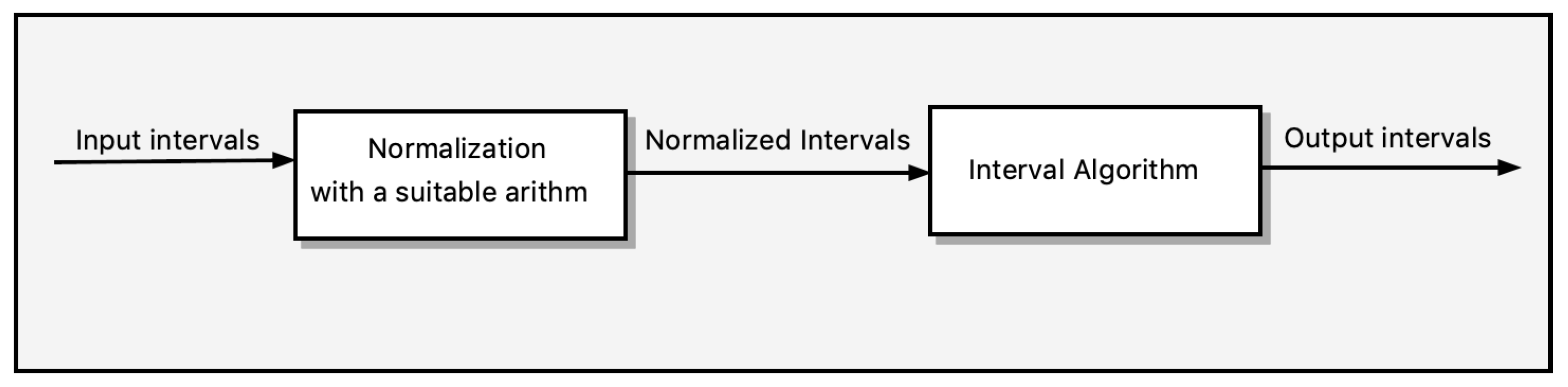
To solve this problem, this paper proposes two axioms that an interval arithmetic must satisfy in order to be applied at the step of normalization. We think that the normalization must be done separately from the rest of the computation without the introduction of uncertainty, since it is just translation of input data. So, any arithmetic applied in such process must satisfy the axioms proposed here—see Figure 1.

The normalization involves division, and division is always faced as an operation having a connection with multiplication (as the inverse operation of that). This viewpoint comes from our experience with numbers. However, this approach has not been sustainable whenever we deal with entities representing uncertainty. For intervals, the usual division does not satisfy the whole properties that connect real division to multiplication. In fact, some interval arithmetics were developed to recover this relation and the benefits that come with the algebraic method—see, for example, [4,5,6,7]. The same situation occurs when we take into account the usual division for fuzzy numbers. Therefore, the notion of interval division requires a careful reflection. In the sequel (Section 2), we show the close relation between the notions of division, partition and normalization. This will be the basis to propose our axioms.

We organized this paper in the following way: Section 2 introduces the notion of Partition Principle (PP), which is an intuitive principle that is realized by the normalization of numbers and by other contexts. We also introduce the notion of Interval Division Structures (IDS), which will be interval structures that satisfy the (PP). Section 3 investigates some known arithmetics and shows if they fit in our axiomatic system. Section 4 provides some consideration on Constrained Interval Arithmetic (CIA) with respect to its approach strongly related with methods of optimization. Finally, Section 5 shows that until now we do not have a universal representation for intervals that is fast to compute and promotes a good division able to capture the notion of data normalization. That section ends by proposing a change in the usual paradigm of interval computation.

2. Partition Principle and Interval Normalization

The literature offers a plethora of interval arithmetics. Some of them intend to recover the algebraic structure of real numbers. Like real numbers, which are seen as representing quantities, measures, and vectors, intervals also have different viewpoints. They are seen as sets, numbers, information about real numbers and real numbers with imprecision [8]. This last viewpoint lead us to see that the “introduction” of imprecision on real numbers induces the loss of field properties of some arithmetics.

Until now interval division has been faced as part of a whole interval arithmetic and has not been faced separately. In other words, the authors have followed the tradition to define the four basic operations and verify the properties of division with respect to the whole arithmetic; mainly that division is connected to multiplication.

However, observe the following notion of division:

Real Numbers

(PP) is perfectly captured by the division on real numbers since for a finite set of reals: $A=\{r_1,\dots ,r_n\}$, s.t. $r_j\ne 0$,

$$\frac{r_1}{{\displaystyle \sum _{j=1}^n}{r}_j}+\dots +\frac{r_n}{{\displaystyle \sum _{j=1}^n}{r}_j}=1.$$

(1)

The “‘partition”, here, is represented by the set $\left\{\frac{r_1}{{\displaystyle \sum _{j=1}^n}{A}_j},\dots ,\frac{r_n}{{\displaystyle \sum _{j=1}^n}{A}_j}\right\}$, the “whole” is numerically represented by “1” and “to collect” means “to sum”.

Example 1.

For the set of real numbers: $A=\{-3,4,7\}$, the division of real numbers provides the partition: $\{\frac{-3}{8},\frac{4}{8},\frac{7}{8}\}$ and $\frac{-3}{8}+\frac{4}{8}+\frac{7}{8}=1$.

Sets

A finite partition of a set X is a family of non-empty pairwise disjoint subsets $A=\{A_1,\dots ,A_n\}$, the union of which recovers X. The “whole” is the set X and “to collect” means to provide the union of sets in the partition: ${\displaystyle \bigcup _{i=1}^n}{A}_i=X$.

Example 2.

Let $X=\{a,b,c,d,e\}$, the family of sets $A=\left\{\right\{a\},\{b,c\},\{d,e\left\}\right\}$ is a partition of X.

Both examples satisfy (PP). In the case of numbers, the “whole” is always represented by the number one. In the case of sets, the whole is represented by the considered universe set X. What about intervals?

As we have stated, interval division has not been defined in this way, but it has been faced as part of an interval arithmetic with some properties. Instead, in what follows we provide an axiomatic system for interval division, which is based on (PP) and investigate how some operations in the literature behaves with respect to such axioms. Before we proceed, we recall the following definitions.

Definition 1

([9]). Given a set A, $x,e\in A$ and an associative operation $\oplus :A\times A\to A$. If $x\oplus e=e\oplus x=x$, then the structure $\langle A,\oplus ,e\rangle$ is called a monoid.

Definition 2

([10]). The set $[a,b]=\{x:\mathbb{R}\mid a\le x\le b\}$ is called the closed interval between a and b. The set of all such intervals is denoted by $\mathbb{I(R)}$. Given an interval $[a,b]\in \mathbb{I(R)}$, the width of $[a,b]$ is $w\left(\right[a,b\left]\right)=b-a$.

Interval Division Structures

In this section we introduce the notion of interval structures that interpret the partition principle (PP). They are called Interval Division Strutures (IDS) and are our proposal to perform the normalization of interval data.

Definition 3.

(Interval Division Structures) A triple $\langle \mathbb{I(R)},\oplus ,\rangle$ is calledinterval division structure (IDS)if $\langle \mathbb{I(R)},\oplus ,[0,0]\rangle$ is a monoid and the following properties are satisfied:

(D-1) Given a finite family of intervals $A=\{A_1,\dots ,A_n\}$ such that $0\notin (A_1\oplus \dots \oplus A_n)$,

$$1\in N\left(A\right)=\left(A_1⨸{\displaystyle \sum _{j=1}^n}{A}_j\right)\oplus \dots \oplus \left(A_n⨸{\displaystyle \sum _{j=1}^n}{A}_j\right).$$

(2)

(D-2)$w\left(N\left(A\right)\right)\le {\displaystyle \sum _{j=1}^n}w\left(A_j\right)$, for all $1\le j\le n$.

The first axiom states that the division must be able to provide an interval that contains the normalization of the numbers contained in each $A_i$.

The second axiom generalizes the standard notion of normalization of real numbers because, since real numbers can be seen as degenerate intervals, Equation (1) is an instance of (D-2). Moreover, (D-2) establishes a relation between the impreciseness of input data and that produced by division; namely, the second should not exceed the first. In other words, the normalization of interval data should not introduce additional impreciseness.

In what follows we show how some interval divisions behave with respect to the axioms of IDS. That is, we will check whether they can be used to normalize data according to our interpretation.

3. Interval Division Structures and Some Interval Artithmetic

In this section we show how some interval sums and divisions behave with respect to the proposed axiomatic system. An interval, X, will be denoted by $X=[\underline{x},\overline{x}]$.

3.1. Standard Interval Arithmetic-SIA

The standard interval sum and division [11] are given by:

$$X+Y=[\underline{x}+\underline{y},\overline{x}+\overline{y}],$$

(3)

and for $\delta =\left\{(\underline{x}/\underline{y}),(\underline{x}/\overline{y}),(\overline{x}/\underline{y}),(\overline{x}/\overline{y})\right\}$ and $0\notin Y$,

$$X/Y=[min(\delta ),max(\delta \left)\right].$$

(4)

It is not hard to prove that (D-1) is valid for SIA. However, SIA does not satisfy (D2). Consider $X_1=[1/12,5/12]$ and $X_2=[1/8,3/8]$. As we can see, $N\left(A\right)=\frac{X_1}{X_1+X_2}+\frac{X_2}{X_1+X_2}=[0.26315,3.8001]$. Thus, $w\left(N\left(A\right)\right)=3.5368>0.58333=w\left(X_1\right)+w\left(X_2\right)$.

The standard interval operations produce wider error bound whenever the same interval appears more than once in an interval expression—for example, $X-X$ or $(X·Y)+(X·Z)$—in both cases the interval X appears more than once and the resulting evaluated interval is wider than the direct image, respectively: $[0,0]$ and $X·(Y+Z)$. This is called the variable dependence problem (VDP) [12], which means that each occurrence of a variable (independent of the expression) influences on the output precision. For instance, consider $X=[1,2],Y=[2,3]$ and $Z=[-1,4]$. Then $X-X=[-1,1]$, $X(Y+Z)=[1,14]$ and $XY+XZ=[0,14]$, hence $X-X\ne 0$ and $X(Y+Z)\subseteq XY+XZ$ (subdistributivity). One can go further, consider $f\left(x\right)=(x+1)(x-1)$, note that $-1\le f\left(x\right)\le 3$ if $x\in [-2,1]$. But $f\left(\right[-2,2\left]\right)=\left(\right[-2,1]+1)\left(\right[-2,1]-1)=[-1,2][-3,-2]=[-6,3]$.

In order to overcome (VDP) some further interval arithmetics were proposed [12]. In what follows we briefly present the sum and division of some arithmetics and show if they satisfy or not our axioms.

3.2. Alberth’s Range Arithmetic

O. Aberth’s Range arithmetic [13] (pp. 13–25) introduces the notion of range number. A range number is an entity of the form: $X=m\pm ϵ$. In fact, it can be seen as an interval $X=[\underline{x},\overline{x}]$, where $m=\frac{\underline{x}+\overline{x}}{2}$ and $ϵ=\frac{\overline{x}-\underline{x}}{2}$. For $X=m_1\pm {ϵ}_1$ and $Y=m_2\pm {ϵ}_2$, the sum is defined by:

$$X+Y=(m_1+m_2)\pm ({ϵ}_1+{ϵ}_2).$$

(5)

This sum coincides with the usual interval sum: $X+Y=[\underline{x}+\underline{y},\overline{x}+\overline{y}]$. The division is given by:

$$X÷Y=(m_1\pm {ϵ}_1)÷(m_2\pm {ϵ}_2)\subseteq \left(\frac{m_1}{m_2}\right)\pm \left(\frac{{ϵ}_1+\mid \frac{m_1}{m_2}\mid {ϵ}_2}{\mid m_2\mid -{ϵ}_2}\right).$$

(6)

Consider $X_1=[1/12,5/12]$ and $X_2=[1/8,3/8]$. Thus, $X_1=\frac{1}{4}\pm \frac{1}{6}$ and $X_2=\frac{1}{4}\pm \frac{1}{8}$.

$N\left(A\right)=\frac{X_1}{X_1+X_2}+\frac{X_1}{X_1+X_2}=(\frac{1}{2}\pm \frac{7}{5})+(\frac{1}{2}\pm \frac{13}{10})=1\pm \frac{24}{5}$,

$w\left(N\left(A\right)\right)=\frac{24}{5}>\frac{7}{24}=\frac{1}{6}+\frac{1}{8}=w\left(X_1\right)+w\left(X_2\right)$.

Therefore this arithmetic will not satisfy the axiom (D-2).

3.3. Hansen’s or Generalized Approach

In 1975 E.R. Hansen [5] proposed a representation for intervals together with an arithmetic. The idea was to maintain “registered” the imprecision of each input interval until the end of the computation and to use it to provide the computation’s output in the standard interval form. In what follows, we use the notation proposed by Hansen in [5].

Given n input intervals: $X_1,\dots ,X_n$ with $j\in \{1,\dots ,n\}$, midpoints $m_j$ and width $w_j$, let be $s_j=\frac{w_j}{2}$ and $U_j=[-s_j,s_j]$. Assuming the standard interval arithmetic, each interval $X_j$ is represented in Generalized Interval Arithmetic (GIA) form in the following way:

$$X_j=A_0^j+{\displaystyle \sum _{r=1}^n}{A}_r^j·U_r,$$

(7)

where $A_0^j=m_j$ and $U_j=[-s_j,s_j]$. Note that $A_k^j$ (for $k>0$) are intervals and $(A_n^j·U_n)$ is the standard interval multiplication. If $X_j$ is an input interval, then $A_k^j=[1,1]$ (for $j=k$) and $A_k^j=[0,0]$ otherwise.

Example 3.

Given the intervals: $X_1=[1,2],X_2=[5,10]$ and $X_3=[-4,-1]$, since we are considering three intervals, their GIA representation is:

$$\begin{array}{cc}\hfill X_1=\stackrel{A_0^1}{\overbrace{1.5}}& +\stackrel{A_1^1}{\overbrace{[1,1]}}·\stackrel{U_1}{\overbrace{[-0.5,0.5]}}+\stackrel{A_2^1}{\overbrace{[0,0]}}·\stackrel{U_2}{\overbrace{[-2.5,2.5]}}\hfill \\ \hfill & +\stackrel{A_3^1}{\overbrace{[0,0]}}·\stackrel{U_3}{\overbrace{[-1.5,1.5]}}.\hfill \\ \hfill X_2=\stackrel{A_0^2}{\overbrace{7.5}}& +\stackrel{A_1^2}{\overbrace{[0,0]}}·\stackrel{U_1}{\overbrace{[-0.5,0.5]}}+\stackrel{A_2^2}{\overbrace{[1,1]}}·\stackrel{U_2}{\overbrace{[-2.5,2.5]}}\hfill \\ \hfill & +\stackrel{A_3^2}{\overbrace{[0,0]}}·\stackrel{U_3}{\overbrace{[-1.5,1.5]}}.\hfill \\ \hfill X_3=\stackrel{A_0^3}{\overbrace{-2.5}}& +\stackrel{A_1^3}{\overbrace{[0,0]}}·\stackrel{U_1}{\overbrace{[-0.5,0.5]}}+\stackrel{A_2^3}{\overbrace{[0,0]}}·\stackrel{U_2}{\overbrace{[-2.5,2.5]}}\hfill \\ \hfill & +\stackrel{A_3^3}{\overbrace{[1,1]}}·\stackrel{U_3}{\overbrace{[-1.5,1.5]}}.\hfill \end{array}$$

The generalized interval arithmetic will produce new intervals with new $A_j^i$’s with the same $U_i$’s.

3.3.1. Addition and Difference

The addition of n generalized intervals according to Equation (7) is given by:

$${\displaystyle \sum _{j=1}^n}{X}_j={\displaystyle \sum _{j=1}^n}{A}_0^j+{\displaystyle \sum _{r=1}^n}\left({\displaystyle \sum _{j=1}^n}{A}_r^j\right)·U_r.$$

(8)

The difference is given by:

$$X_k-X_j=(A_0^k-A_0^j)+{\displaystyle \sum _{r=1}^n}(A_r^k-A_r^j)·U_r$$

(9)

Example 4.

Assuming the previous intervals, let’s calculate $(X1+X3)+(X2-X1)$.

$$\begin{array}{c}\hspace{1em}\hspace{1em}(X_1+X_3)\equiv \stackrel{A_0^1+A_0^3}{\overbrace{1.5+(-2.5)}}+\stackrel{A_1^1+A_1^3}{\overbrace{[1,1]+[0,0]}}·\stackrel{U_1}{\overbrace{[-0.5,0.5]}}+\stackrel{A_2^1+A_2^3}{\overbrace{[0,0]+[0,0]}}·\stackrel{U_2}{\overbrace{[-2.5,2.5]}}+\\ +\stackrel{A_3^1+A_3^3}{\overbrace{[0,0]+[1,1]}}·\stackrel{U_3}{\overbrace{[-1.5,1.5]}}.\end{array}$$

Therefore, $X_1+X_3\equiv -1+[1,1]·U_1+[0,0]·U_2+[1,1]·U_3$. Similarly $X_2-X_1=6+[-1,-1]·U_1+[1,1]·U_2+[0,0]·U_3$ and $(X1+X3)+(X2-X1)=5+[0,0]·U_1+[1,1]·U_2+[1,1]·U_3$.

Before we proceed, let us see how we recover the standard form of an interval: Take the generalized form, substitute each $U_j$ in the expression and apply the standard interval arithmetic. For example: $X_1=(1.5+[1,1]·U1+[0,0]·U_2+[0,0]·U_3)=(1.5+[1,1]·[-0.5,0.5]+[0,0]·[-2.5,2.5]+[0,0]·[-1.5,1.5])=1.5+[-0.5,0.5]=[1,2]$.

Similarly, $X_2-X_1=6+[-1,-1]·U_1+[1,1]·U_2+[0,0]·U_3=6+[-0.5,0.5]+[-2.5,2.5]=[3,9]$. Observe that in this case “$X_2-X_1$” coincides with the standard approach. However, whereas $X_2-X_2=[-5,5]$ with standard arithmetic, for any interval X, GIA provides: $X-X=[0,0]$.

3.3.2. Division

The division of two generalized intervals is given by:

$$\frac{X_i}{X_j}=\left(\frac{A_0^i}{A_0^j}\right)+{\displaystyle \sum _{r=1}^n}\left(Z_r·U_r\right)$$

(10)

where

$$Z_r=\frac{A_0^j·A_r^i-A_0^i·A_r^j}{K},\mathrm{for}K=A_0^j\left(A_0^j+{\displaystyle \sum _{s=1}^n}{A}_s^j·U_s\right).$$

Example 5.

Now, for simplicity, consider just $X_2$ and $X_3$, then:

$$\begin{array}{cc}\hfill X_2=\stackrel{A_0^2}{\overbrace{7.5}}& +\stackrel{A_1^2}{\overbrace{[1,1]}}·\stackrel{U_1}{\overbrace{[-2.5,2.5]}}+\stackrel{A_2^2}{\overbrace{[0,0]}}·\stackrel{U_2}{\overbrace{[-1.5,1.5]}},\hfill \\ \hfill X_3=\stackrel{A_0^3}{\overbrace{-2.5}}& +\stackrel{A_1^3}{\overbrace{[0,0]}}·\stackrel{U_1}{\overbrace{[-2.5,2.5]}}+\stackrel{A_2^3}{\overbrace{[1,1]}}·\stackrel{U_2}{\overbrace{[-1.5,1.5]}}.\hfill \end{array}$$

Therefore, $K=A_0^3(A_0^3+A_1^3·U_1+A_2^3·U_2)$, $Z_{K1}\stackrel{def}{=}\left(\frac{A_0^3·A_1^2-A_0^2·A_1^3}{K}\right)=[-1,-0.25]$ and $Z_{K2}\stackrel{def}{=}\left(\frac{A_0^3·A_2^2-A_0^2·A_2^3}{K}\right)=[-3,-0.75]$. So,

$$\frac{X_2}{X_3}=-\frac{7.5}{2.5}+[-1,-0.25]·U_1+[-3,-0.75]·U_2.$$

Proposition 1.

Let $A=\{X_1,\dots ,X_n\}$ be a family of intervals s.t.

$${\displaystyle X_j=A_0^j+{\displaystyle \sum _{r=1}^n}\left(A_r^j·U_r\right),}$$

(where $A_i^j=0$ if $i\ne j$ and $A_i^j=1$ if $i=j$) and ${\displaystyle D=\left({\displaystyle \sum _{k=0}^n}{A}_0^k\right)\left({\displaystyle \sum _{k=0}^n}{A}_0^k+[-1,1]{\displaystyle \sum _{k=0}^n}\frac{w\left(X_k\right)}{2}\right)}$. Then we can write:

$${\displaystyle N\left(A\right)=1+{\displaystyle \sum _{m=1}^n}\left(U_m·{\displaystyle \sum _{k=1,k\ne m}^n}{A}_0^k\left(\frac{1}{D}-\frac{1}{D}\right)\right).}$$

Proof. 

According to Equation (10) one can write:

$$\frac{X_i}{X_1+\cdots +X_n}=\frac{A_0^i}{A_0^1+\cdots +A_0^n}+{\displaystyle \sum _{r=1}^n}\left(Z_r^i·U_r\right),$$

where

$$Z_r^i=\frac{(A_0^1+\cdots +A_0^n)·A_r^i-A_0^i·(A_r^1+\cdots +A_r^n)}{(A_0^1+\cdots +A_0^n)·((A_0^1+\cdots +A_0^n)+{\sum }_{s=1}^n(A_s^1+\cdots +A_s^n)U_s)}$$

$$=\frac{(A_0^1+\cdots +A_0^n)·A_r^i-A_0^i·(A_r^1+\cdots +A_r^n)}{D}.$$

Remember that, $A_i^j=0$ if $i\ne j$ and $A_i^j=1$ if $i=j$. Hence,

$Z_r^i=\frac{-A_0^i}{D}$ if $i\ne r$ and $Z_r^i=\frac{{\displaystyle {\displaystyle \sum _{k=1,k\ne i}^n}{A}_0^k}}{D}$ if $i=r$. Thus,

$\frac{X_i}{X_1+\cdots +X_n}=\frac{A_0^i}{A_0^1+\cdots +A_0^n}+\cdots +\frac{{\displaystyle {\displaystyle \sum _{k=1,k\ne i}^n}{A}_0^k}}{D}{U}_i+\cdots +\frac{-A_0^i}{D}{U}_1.$

Thus,

$$\frac{X_1}{X_1+\cdots +X_n}=\frac{A_0^1}{A_0^1+\cdots +A_0^n}+\frac{{\displaystyle {\displaystyle \sum _{k=1,k\ne 1}^n}{A}_0^k}}{D}{U}_1+\frac{-A_0^1}{D}{U}_2+\cdots +\frac{-A_0^1}{D}{U}_n,$$

$$\frac{X_2}{X_1+\cdots +X_n}=\frac{A_0^2}{A_0^1+\cdots +A_0^n}+\frac{-A_0^2}{D}{U}_1+\frac{{\displaystyle {\displaystyle \sum _{k=1,k\ne 2}^n}{A}_0^k}}{D}{U}_2+\cdots +\frac{-A_0^2}{D}{U}_n,$$

$$⋮$$

$$\frac{X_n}{X_1+\cdots +X_n}=\frac{A_0^n}{A_0^1+\cdots +A_0^n}+\frac{-A_0^n}{D}{U}_1+\frac{-A_0^n}{D}{U}_2+\cdots +\frac{{\displaystyle {\displaystyle \sum _{k=1,k\ne n}^n}{A}_0^k}}{D}{U}_n.$$

Hence,

$$\begin{array}{cc}\hfill N\left(A\right)& =\frac{X_1}{X_1+\cdots +X_n}+\cdots +\frac{X_n}{X_1+\cdots +X_n}\hfill \\ & =\frac{A_0^1+\cdots +A_0^n}{A_0^1+\cdots +A_0^n}+\left({\displaystyle \sum _{k=1,k\ne 1}^n}\left(\frac{A_0^k}{D}-\frac{A_0^k}{D}\right)\right)U_1+\cdots +\left({\displaystyle \sum _{k=1,k\ne n}^n}\left(\frac{A_0^k}{D}-\frac{A_0^k}{D}\right)\right)U_n\hfill \\ & =1+\left({\displaystyle \sum _{k=1,k\ne 1}^n}{A}_0^k\left(\frac{1}{D}-\frac{1}{D}\right)\right)U_1+\cdots +\left({\displaystyle \sum _{k=1,k\ne n}^n}{A}_0^k\left(\frac{1}{D}-\frac{1}{D}\right)\right)U_n\hfill \\ & =1+{\displaystyle \sum _{m=1}^n}\left(U_m·{\displaystyle \sum _{k=1,k\ne m}^n}{A}_0^k\left(\frac{1}{D}-\frac{1}{D}\right)\right).\hfill \end{array}$$

□

Corollary 1.

Consider a family of intervals $\{X_1,\dots ,X_n\}$ where $X_j=A_0^j+{\sum }_{r=1}^n(A_r^j·U_r)$. Then $1\in N\left(A\right)$, i.e., Hansen’s division satisfies (D-1).

Proof. 

Note that $U_j$ and $A_0^j\left(\frac{1}{D}-\frac{1}{D}\right)$ are symmetric intervals for $j=1,\dots n$. Thus, ${\sum }_{m=1}^n\left(U_m·{\sum }_{k=1,k\ne m}^n{A}_0^k\left(\frac{1}{D}-\frac{1}{D}\right)\right)$ is a symmetric interval. Therefore

$$1+{\displaystyle \sum _{m=1}^n}\left(U_m·{\displaystyle \sum _{k=1,k\ne m}^n}{A}_0^k\left(\frac{1}{D}-\frac{1}{D}\right)\right)$$

contains 1. □

Remark 1.

The impact of variable dependence is weaker with the GIA than with the SIA, however its sum together with division fails to be an interval division structure. Observe the following example:

Example 6.

Consider $X_1=\left[\frac{1}{12},\frac{5}{12}\right]$ and $X_2=\left[\frac{1}{8},\frac{3}{8}\right]$. Using only $X_1$ and $X_2$ in Hansen’s representation, according to Equation (7) and by Corollary 1, the Hansen division satisfies (D-1) but does not satisfy (D-2):

$$X_1=\stackrel{A_0^1}{\overbrace{\frac{1}{4}}}+\stackrel{A_1^1}{\overbrace{\left[1,1\right]}}·\stackrel{U_1}{\overbrace{\left[-\frac{1}{6},\frac{1}{6}\right]}}+\stackrel{A_2^1}{\overbrace{\left[0,0\right]}}·\stackrel{U_2}{\overbrace{\left[-\frac{1}{8},\frac{1}{8}\right]}}$$

$$and$$

$$X_2=\stackrel{A_0^2}{\overbrace{\frac{1}{4}}}+\stackrel{A_1^2}{\overbrace{\left[0,0\right]}}·\stackrel{U_1}{\overbrace{\left[-\frac{1}{6},\frac{1}{6}\right]}}+\stackrel{A_2^2}{\overbrace{\left[1,1\right]}}·\stackrel{U_2}{\overbrace{\left[-\frac{1}{8},\frac{1}{8}\right]}}$$

To apply Proposition 1 consider

$$\begin{array}{cc}\hfill D& =(A_0^1+A_0^2)\left(A_0^1+A_0^2+\left[-1,1\right]\left(\frac{w\left(X_1\right)}{2}+\frac{w\left(X_2\right)}{2}\right)\right)\hfill \\ & =\left(\frac{1}{4}+\frac{1}{4}\right)\left(\frac{1}{4}+\frac{1}{4}+\left[-1,1\right]\left(\frac{1}{6}+\frac{1}{8}\right)\right)\hfill \\ \hfill & =\left[\frac{5}{48},\frac{19}{48}\right].\hfill \end{array}$$

Thus $\frac{1}{D}=\left[\frac{48}{19},\frac{48}{5}\right]$ and $\left(\frac{1}{D}-\frac{1}{D}\right)=\left[-\frac{672}{95},\frac{672}{95}\right]$. Now we can evaluate $N\left(A\right)$ as follows:

$$\begin{array}{cc}\hfill N\left(A\right)& =1+U_1{A}_0^2\left(\frac{1}{D}-\frac{1}{D}\right)+U_2{A}_0^1\left(\frac{1}{D}-\frac{1}{D}\right)\hfill \\ & =1+\left[-\frac{1}{6},\frac{1}{6}\right]\frac{1}{4}\left[-\frac{672}{95},\frac{672}{95}\right]+\left[-\frac{1}{8},\frac{1}{8}\right]\frac{1}{4}\left[-\frac{672}{95},\frac{672}{95}\right]\hfill \\ & =[0.48421,1.5158].\hfill \end{array}$$

Then $w\left(N\left(A\right)\right)=1.0316>0.583333=w\left(X_1\right)+w\left(X_2\right)$. Therefore, Hansen’s sum and division do not provide an IDS.

3.4. Affine Arithmetic

Developed by Jorge Stolfi and Luiz Figueiredo [4,14], Affine arithmetic (AA) is a method proposed to overcome the overestimation. The ideal quantities are represented by affine forms. Each AA operation provides a framework in which the approximation errors have, normally, a quadratic dependency with respect to width of the input intervals even when the operands are correlated, for example, in $X·(1-X)$. Thus, for tight input intervals, the operations provide tight estimations of the exact range.

In AA, a quantity x is written by an affine form:

$$\widehat{x}=x_0+x_1{ϵ}_1+\cdots +x_n{ϵ}_n.$$

The coefficients $x_i$ are finite floating-point numbers and the ${ϵ}_i$ are symbolic real variables, the values of which are unknown but assumed to lie in the interval $\mathbb{U}=[-1,+1]$. The value $x_0$ is called central value of $\widehat{x}$, whereas each coefficient $x_i$ is called a partial deviation. Finally, each ${ϵ}_i$ represents noise.

Each affine expression $\widehat{x}=x_0+x_1{ϵ}_1+\cdots +x_n{ϵ}_n$ implies an interval bound for the corresponding ideal quantity x, namely $x\in X=[x_0-s,x_0+s]$, where ${\displaystyle s={\displaystyle \sum _{i=1}^n}\left|x_i\right|}$ is the total deviation of $\widehat{x}$. Conversely, every interval $X=[a,b]$ representing a real number x can be written as an affine form $\widehat{x}=x_0+x_k{ϵ}_k$ s.t.: $x_0$ is the midpoint $\frac{a+b}{2}$, $x_k=\frac{b-a}{2}$, and ${ϵ}_k$ is a new symbol for noise—i.e., it does not occur in any other existing affine expression.

This is very important, since some operations—even one primitive arithmetical operation—will require this resource. Those operations are classified as non-affine operations and are described in [4] (p. 53).

Affine Arithmetic: Given $\widehat{x}=x_0+x_1{ϵ}_1+\cdots +x_n{ϵ}_n$ and $\widehat{y}=y_0+y_1{ϵ}_1+\cdots +y_n{ϵ}_n$. According to [4,14]:

• $\widehat{x}\pm \widehat{y}=(x_0\pm y_0)+(x_1\pm y_1){ϵ}_1+\cdots +(x_n\pm y_n){ϵ}_n$.
• $\widehat{x}·\widehat{y}=(x_0+x_1{ϵ}_1+\cdots +x_n{ϵ}_n)·(y_0+y_1{ϵ}_1+\cdots +y_n{ϵ}_n)$.
• $\frac{\widehat{x}}{\widehat{y}}=\widehat{x}·\frac{1}{\widehat{y}}$, where the inverse function $\frac{1}{\widehat{y}}$ is computed by replacing $\widehat{y}$ with its corresponding interval, denoted $\left[\widehat{y}\right]$ (see the routine in [4] (p. 70)). Thus, the reciprocal is obtained by (1) converting the affine form onto the standard form, (2) applying the standard/usual interval arithmetic and (3) converting back the resulting interval into the corresponding affine form to proceed with the computation.

Like Hansen’s approach, Affine arithmetic does not provide an IDS, since (D-2) is not satisfied:

Example 7.

Consider $X_1=[1/12,5/12]$ and $X_2=[1/8,3/8]$. Thus, ${\widehat{x}}_1=\frac{1}{4}+\frac{1}{6}{ϵ}_1$ and ${\widehat{x}}_2=\frac{1}{4}+\frac{1}{8}{ϵ}_2$. Evaluating:

$$\begin{array}{cc}\hfill \frac{{\widehat{x}}_1}{{\widehat{x}}_1+{\widehat{x}}_2}& =\frac{\frac{1}{4}+\frac{1}{6}{ϵ}_1}{\frac{1}{2}+\frac{1}{6}{ϵ}_1+\frac{1}{8}{ϵ}_2}\hfill \\ \hfill & =\left(\frac{1}{4}+\frac{1}{6}{ϵ}_1\right)·\frac{1}{\left[\frac{5}{24},\frac{19}{24}\right]}\hfill \\ \hfill & =\left(\frac{1}{4}+\frac{1}{6}{ϵ}_1\right)·\left[\frac{24}{19},\frac{24}{5}\right]\hfill \\ \hfill & =\left(\frac{1}{4}+\frac{1}{6}{ϵ}_1\right)·\left(\frac{288}{95}+\frac{168}{95}{ϵ}_3\right)\hfill \\ \hfill & =\frac{72}{95}+\frac{144}{285}{ϵ}_1+\frac{42}{95}{ϵ}_3+\frac{84}{285}{ϵ}_1{ϵ}_3,\hfill \end{array}$$

and in the same way,

$$\begin{array}{cc}\hfill \frac{\widehat{x_2}}{\widehat{x_1}+\widehat{x_2}}& =\frac{72}{95}+\frac{36}{95}{ϵ}_2+\frac{42}{95}{ϵ}_3+\frac{21}{95}{ϵ}_2{ϵ}_3.\hfill \end{array}$$

Now,

$N\left(A\right)=\frac{\widehat{x_1}}{\widehat{x_1}+\widehat{x_2}}+\frac{\widehat{x_2}}{\widehat{x_1}+\widehat{x_2}},$

$N\left(A\right)=\frac{144}{95}+\frac{144}{285}{ϵ}_1+\frac{36}{95}{ϵ}_2+\frac{84}{95}{ϵ}_3+\frac{84}{285}{ϵ}_1{ϵ}_3+\frac{21}{95}{ϵ}_2{ϵ}_3.$

As we know, ${ϵ}_1,{ϵ}_2,{ϵ}_3\in [-1,1]$ and the following form $\frac{84}{285}{ϵ}_1{ϵ}_3+\frac{21}{95}{ϵ}_2{ϵ}_3$ has the best approximation on min/max on $[-1,1]\times [-1,1]$ as $[a,b]=\left[-\frac{49}{95},\frac{49}{95}\right]$. According to [4,14] we have:

$$\begin{array}{cc}\hfill N\left(A\right)& =\frac{144}{95}+\frac{144}{285}{ϵ}_1+\frac{36}{95}{ϵ}_2+\frac{84}{95}{ϵ}_3+\left(\left(\frac{a+b}{2}\right)+\left(\frac{b-a}{2}\right)\right){ϵ}_4\hfill \\ & =\frac{144}{95}+\frac{144}{285}{ϵ}_1+\frac{36}{95}{ϵ}_2+\frac{84}{95}{ϵ}_3+\frac{49}{95}{ϵ}_4\hfill \\ & =\left[-\frac{73}{95},\frac{361}{95}\right].\hfill \end{array}$$

Therefore $w\left(N\left(A\right)\right)=\frac{288}{95}>0.583333=w\left({\widehat{x}}_1\right)+w\left({\widehat{x}}_2\right)$.

3.5. Generalized Hukuhara’s Division

The usual interval arithmetic produces some particular issues, for instance, we can find intervals, $X,Y$ and Z, s.t. $(X+Y)-Y\ne X$. To overcome this problem, Hukuhara [15] proposed a new difference for intervals, called H-difference:

$$(X{\displaystyle \stackrel{H}{\ominus }}Y)=Z\iff X=(Y+Z).$$

(11)

An important property of this difference is that $X{\displaystyle \stackrel{H}{\ominus }}X=[0,0]$ and $(X+Y)-Y=X$. Although this difference provides a unique value it is a partial function. For example the difference, $[3,4]{\displaystyle \stackrel{H}{\ominus }}[2,5]$, is not defined since the resulting value should be $[1,-1]$, which is not an interval. In order to extend this operation to a total one, Stefanini [6] proposed the generalized difference:

$$(X{\displaystyle \stackrel{G}{\ominus }}Y)=Z\iff \left\{\begin{array}{c}\left(\mathrm{i}\right) X=(Y+Z),\hfill \\ \mathrm{or} \left(\mathrm{ii}\right) Y=X+(-1)·Z.\hfill \end{array}\right.$$

(12)

In the same way, Stefanini proposed a generalized division:

$$\left(X{÷}_{g}Y\right)=Z\iff \left\{\begin{array}{c}\left(\mathrm{i}\right) X=(Y·Z),\hfill \\ \mathrm{or} \left(\mathrm{ii}\right) Y=(X·Z^{-1}).\hfill \end{array}\right.$$

(13)

For $X=[\underline{x},\overline{x}]$ and $Y=[\underline{y},\overline{y}]$, s.t. $0\notin (\underline{y},\overline{y})$, $X{÷}_{g}Y=Z$ can be evaluated according to the following rules:

- Case 1: If $0<\underline{x}$ and $\overline{y}<0$, then:

If $\underline{x}·\underline{y}\ge \overline{x}·\overline{y}$, then ${\displaystyle \underline{z}=\frac{\overline{x}}{\underline{y}}}$ and ${\displaystyle \overline{z}=\frac{\underline{x}}{\overline{y}}}$.

If $\underline{x}·\underline{y}\le \overline{x}·\overline{y}$, then ${\displaystyle \underline{z}=\frac{\underline{x}}{\overline{y}}}$ and ${\displaystyle \overline{z}=\frac{\overline{x}}{\underline{y}}}$.

- Case 2: If $0<\underline{x}$ and $0<\underline{y}$, then:

If $\underline{x}·\overline{y}\le \overline{x}·\underline{y}$, then ${\displaystyle \underline{z}=\frac{\underline{x}}{\underline{y}}}$ and ${\displaystyle \overline{z}=\frac{\overline{x}}{\overline{y}}}$.

If $\underline{x}·\overline{y}\ge \overline{x}·\underline{y}$, then ${\displaystyle \underline{z}=\frac{\overline{x}}{\overline{y}}}$ and ${\displaystyle \overline{z}=\frac{\underline{x}}{\underline{y}}}$.

- Case 3: If $\overline{x}<0$ and $\overline{y}<0$, then:

${\displaystyle \underline{z}=\frac{\overline{x}}{\overline{y}}}$ and ${\displaystyle \overline{z}=\frac{\underline{x}}{\underline{y}}}$ whenever $\overline{x}·\underline{y}\le \underline{x}·\overline{y}$.

${\displaystyle \underline{z}=\frac{\underline{x}}{\underline{y}}}$ and ${\displaystyle \overline{z}=\frac{\overline{x}}{\overline{y}}}$ whenever $\overline{x}·\underline{y}\ge \underline{x}·\overline{y}$.

- Case 4: If $\overline{x}<0$ and $0<\underline{y}$, then:

If $\underline{x}·\underline{y}\le \overline{x}·\overline{y}$, then ${\displaystyle \underline{z}=\frac{\underline{x}}{\overline{y}}}$ and ${\displaystyle \overline{z}=\frac{\overline{x}}{\underline{y}}}$.

If $\underline{x}·\underline{y}\ge \overline{x}·\overline{y}$, then ${\displaystyle \underline{z}=\frac{\overline{x}}{\underline{y}}}$ and ${\displaystyle \overline{z}=\frac{\underline{x}}{\overline{y}}}$.

- Case 5: If $\underline{x}\le 0,\overline{x}\ge 0$ and $\overline{y}<0$, then the solution does not depend on $\overline{y}$, thus:

${\displaystyle \underline{z}=\frac{\overline{x}}{\underline{y}}}$ and ${\displaystyle \overline{z}=\frac{\underline{x}}{\underline{y}}}$.

- Case 6: If $\underline{x}\le 0,\overline{x}\ge 0$ and $0<\overline{y}$, then the solution does not depend on $\underline{y}$, thus:

${\displaystyle \underline{z}=\frac{\underline{x}}{\overline{y}}}$ and ${\displaystyle \overline{z}=\frac{\overline{x}}{\overline{y}}}$.

If $0\in [\underline{y},\overline{y}]$ the generalized division is undefined; for intervals $Y=[0,\overline{y}$] or $Y=[\underline{y},0]$ the division is possible but obtaining unbounded results Z of the form $Z=(-\infty ,\overline{z}]$ or $Z=[\underline{z},+\infty )$.

Proposition 2.

Generalized Hukuhara division is not an IDS.

Proof. 

Consider $X=[-2,-1]$ and $Y=[3,\frac{7}{2}]$. Hence,

$$\begin{array}{cc}\hfill N\left(A\right)& =\frac{X}{X+Y}+\frac{Y}{X+Y}\hfill \\ & =\underset{Case4}{\underbrace{\frac{[-2,-1]}{[1,\frac{5}{2}]}}}+\underset{Case2}{\underbrace{\frac{[3,\frac{7}{2}]}{[1,\frac{5}{2}]}}}\hfill \\ & =\left[-1,-\frac{4}{5}\right]+\left[\frac{7}{5},3\right]\hfill \\ & =\left[\frac{2}{5},\frac{11}{5}\right].\hfill \end{array}$$

Therefore, $w\left(N\left(A\right)\right)=\frac{9}{5}\ge \frac{3}{2}=w\left(X\right)+w\left(Y\right)$. □

3.6. Constrained Arithmetic

The standard approach and its extensions are based on what Lodwick [12] calls the axiomatic approach: The operations are defined in terms of equations that determine how to obtain intervals by the calculation with endpoints. For example, $X+Y=[\underline{x}+\underline{y},\overline{x}+\overline{y}]$.

“The power of the axiomatic approach to interval arithmetic is that it is simple to apply. Its complexity is at most four times that of real-valued arithmetic. However, the axiomatic approach to interval arithmetics leads to overestimations in general because it takes every instantiation of the same variable independently.”

[12]

The most important property for an interval operation is correctness [16]: For a real number x, an interval X, a real operation f and an interval operation F,

$$x\in X\Rightarrow f\left(x\right)\in F\left(X\right).$$

(14)

This can be achieved for interval functions that satisfy the extension principle. It comes from set theory [17] and is simply the application of direct images.

Definition 4.

Given any function, $f:A\to B$, and the powersets $\mathcal{P}\left(A\right)$ and $\mathcal{P}\left(B\right)$, there is a function calleddirect imageof f, $f:\mathcal{P}\left(A\right)\to \mathcal{P}\left(B\right)$, such that $f\left(S\right)=\{f\left(x\right):x\in S\}={\bigcup }_{x\in S}\left\{f\left(x\right)\right\}$.

The direct image is also noted as $\mathcal{P}\left(f\right)$ (see [18] (p. 195 Ex.3)). For the real line, the direct image of continuous functions, $f:{\mathbb{R}}^n\to \mathbb{R}$, always maps closed intervals into closed intervals. In other words, $f\left(\right[a,b\left]\right)=\left\{f\right(x):x\in [a,b\left]\right\}=[c,d]$. Since the operations of real arithmetic are continuous functions, then the definition of interval arithmetic can be expressed in the form:

$$[a,b]\ast [c,d]=\{x\ast y:x\in [a,b] \mathrm{and} y\in [c,d\left]\right\}.$$

(15)

where $\ast \in \{+,-,/,\times \}$. However, this definition imposes all the combinations of elements of both intervals which leads to situations in which $X-X\ne 0$, even when X is representing the same number. This problem of overestimation is solved, for example, by using the Hansen’s approach.

Lodwick [12] proposed another approach called: Constrained Interval Arithmetic (CIA). The idea follows the same approach proposed by some other interval arithmetics (like Range [13] or Hansen/Generalized arithmetics [5]) in which the authors provide another representation form to represent intervals, an arithmetic for such representation and a way to recover the set interpretation of intervals. In the case of the CIA approach, an interval is represented as a function:

Definition 5.

Given an interval $X=[\underline{x},\overline{x}]$ with width, $w_x$, theconstrained function, $X^I:[0,1]\to \mathbb{R}$, related to X is,

$$X^I\left({\lambda }_x\right)=(1-{\lambda }_x)·\underline{x}+\left({\lambda }_x\right)·\overline{x}=\underline{x}+w_x·{\lambda }_x.$$

(16)

These functions are also calledconstrained intervals.

Example 8.

The interval $[3,4]$ is represented by the constrained function: $X^I\left({\lambda }_x\right)=(1-{\lambda }_x)·3+4·{\lambda }_x={\lambda }_x+3$.

Observe that $\underline{x}$ and $\overline{x}$ are known whereas ${\lambda }_x$ is varying.

Definition 6.

Assuming the real operations: $\ast \in \{+,-,/,\times \}$, an arithmetic associated with constrained intervals, calledconstrained interval arithmetic (CIA), is given by:

$$X^I\left({\lambda }_x\right)\ast Y^I\left({\lambda }_y\right),$$

(17)

where the resulting interval, $Z=X\ast Y$, is the set $Z=\{\theta (x,y):0\le {\lambda }_x,{\lambda }_y\le 1\}$, for $\theta (x,y)=\left((1-{\lambda }_x)·\underline{x}+\left({\lambda }_x\right)·\overline{x}\right)\ast \left((1-{\lambda }_y)·\underline{y}+\left({\lambda }_y\right)·\overline{y}\right)$. So,

$$Z=\left[\underset{\mathbf{0}\le {\lambda }_{\mathbf{x}},{\lambda }_{\mathbf{y}}\le \mathbf{1}}{\mathbf{min}}\theta (x,y),\underset{\mathbf{0}\le {\lambda }_{\mathbf{x}},{\lambda }_{\mathbf{y}}\le \mathbf{1}}{\mathbf{max}}\theta (x,y)\right].$$

(18)

The case “$X^I/Y^I$” is undefined whenever $0\in Y$.

Example 9.

For $X=[2,4]$ and $Y=[1,5]$, $X^I=(1-{\lambda }_x)·\underline{x}+\left({\lambda }_x\right)·\overline{x}$ and $Y^I=(1-{\lambda }_y)·\underline{y}+\left({\lambda }_y\right)·\overline{y}$. Let be $\theta (x,y)=X^I+Y^I=(2·{\lambda }_x+2)+(4·{\lambda }_y+1)$. Then, $Z=X+Y=[\underset{\mathbf{0}\le {\lambda }_{\mathbf{x}},{\lambda }_{\mathbf{y}}\le \mathbf{1}}{\mathbf{min}}\theta (x,y),\underset{\mathbf{0}\le {\lambda }_{\mathbf{x}},{\lambda }_{\mathbf{y}}\le \mathbf{1}}{\mathbf{max}}\theta (x,y)]=[3,9]$.

Since the lambdas are connected with the variables in the interval expressions, then $X\ast X=[\underset{\mathbf{0}\le {\lambda }_{\mathbf{x}}\le \mathbf{1}}{\mathbf{min}}\theta (x,x),\underset{\mathbf{0}\le {\lambda }_{\mathbf{x}}\le \mathbf{1}}{\mathbf{max}}\theta ]$, where $\theta (x,x)=\left((1-{\lambda }_x)·\underline{x}+\left({\lambda }_x\right)·\overline{x}\right)\ast \left((1-{\lambda }_x)·\underline{x}+\left({\lambda }_x\right)·\overline{x}\right)$.

Therefore, we have the following properties [12]:

(CIA-1)$X+X=2·X=[2·\underline{X},2·\overline{X}]$,

(CIA-2)$X-X=0$,

(CIA-3)$X÷X=[1,1]$, for $0\notin X$,

(CIA-4)$X·X=[min({\underline{X}}^2,{\overline{X}}^2,0),max({\underline{X}}^2,{\overline{X}}^2,0)]$.

Observe that CIA is an arithmetic in which the evaluation of expressions has a powerful influence on the result. For example, for $X=[1,2]$ and $Y=[-1,1]$, take the interval expression: $X+Y-X$. Then, $X^I\left({\lambda }_x\right)=1·(1-{\lambda }_x)+2{\lambda }_x=$$({\lambda }_x+1)$ and $Y^I\left({\lambda }_y\right)=(-1)·(1-{\lambda }_y)+1·{\lambda }_y=$$(2{\lambda }_y-1)$. The evaluation of the whole expression will lead to Y, since $\theta (x,y)$ is equal to: “$({\lambda }_x+1)+(2{\lambda }_y-1)-({\lambda }_x+1)=(2{\lambda }_y-1)$” and $X+Y-X=[\underset{\mathbf{0}\le {\lambda }_{\mathbf{y}}\le \mathbf{1}}{\mathbf{min}}(2{\lambda }_y-1),\underset{\mathbf{0}\le {\lambda }_{\mathbf{y}}\le \mathbf{1}}{\mathbf{max}}(2{\lambda }_y-1)]=[-1,1]$. However, if we first evaluate $X+Y$, we obtain the interval, $Z=X+Y=[0,3]$, and the respective constrained function: $Z^I=3{\lambda }_z$. Therefore,

$$X+Y-X=Z-X=[\underset{\mathbf{0}\le {\lambda }_{\mathbf{z}},{\lambda }_{\mathbf{x}}\le \mathbf{1}}{\mathbf{min}}3{\lambda }_z-({\lambda }_x+1),\underset{\mathbf{0}\le {\lambda }_{\mathbf{z}},{\lambda }_{\mathbf{x}}\le \mathbf{1}}{\mathbf{max}}3{\lambda }_z-({\lambda }_x+1)]=[-2,2].$$

It is assumed that the whole expression is evaluated before the calculation of min and max.

Proposition 3.

The structure $\langle \mathbb{I(R)},\oplus ,⨸\rangle$, where ⊕ and ⨸ are the CIA addition and division respectively, is an IDS.

Proof. 

The proof is straightforward. For a given finite family of intervals $\{X_1,\dots ,X_n\}$, $N\left(A\right)=[\underset{\mathbf{0}\le {\lambda }_{{\mathbf{x}}_{\mathbf{1}}},\cdots {\lambda }_{{\mathbf{x}}_{\mathbf{n}}}\le \mathbf{1}}{\mathbf{min}}\theta ,\underset{\mathbf{0}\le {\lambda }_{{\mathbf{x}}_{\mathbf{1}}}\cdots {\lambda }_{{\mathbf{x}}_{\mathbf{n}}}\le \mathbf{1}}{\mathbf{max}}\theta ]$, where $\theta :{\mathbb{R}}^n⟶\mathbb{R}$ defined by:

$$\begin{array}{cc}\hfill \theta ({\lambda }_{x_1},\dots ,{\lambda }_{x_n})& =\frac{X_1^I\left({\lambda }_{x_1}\right)}{X_1^I\left({\lambda }_{x_1}\right)+\cdots +X_n^I\left({\lambda }_{x_n}\right)}+\cdots +\frac{X_n^I\left({\lambda }_{x_n}\right)}{X_1^I\left({\lambda }_{x_1}\right)+\cdots +X_n^I\left({\lambda }_{x_n}\right)}\hfill \\ & =\frac{X_1^I\left({\lambda }_{x_1}\right)+\cdots +X_n^I\left({\lambda }_{x_n}\right)}{X_1^I\left({\lambda }_{x_1}\right)+\cdots +X_n^I\left({\lambda }_{x_n}\right)}\hfill \\ & =1.\hfill \end{array}$$

Thus, $N\left(A\right)=[1,1]$ and $0=w\left(N\left(A\right)\right)\le {\displaystyle \sum _{j=1}^n}w\left(X_j\right)$, for all $0\le j\le n$. Therefore, (D-1) and (D-2) are satisfied. □

4. Some Considerations about CIA

The standard arithmetic (SIA) has a simple application and an irrelevant complexity for modern computers. Nevertheless, SIA produces to overestimation. Refinement of interval extensions is a method for computing arbitrarily sharp upper and lower bounds for the values of a real function (see [19]). As a consequence, the overestimation may be reduced. However, this method becomes too slow if we consider a large interval or complex functions, for instance exponential or trigonometric. On the other hand, constrained interval arithmetic (CIA) [12] overcomes the overestimations and becomes closer to real numbers. As we demonstrated, constrained arithmetic, in particular on division is an IDS, i.e., the overestimation on division is less than the sum of the terms, since D-2 is satisfied. However, in our opinion constrained arithmetic has some issues, for instance every operation needs to optimize a specific function, consider the following example:

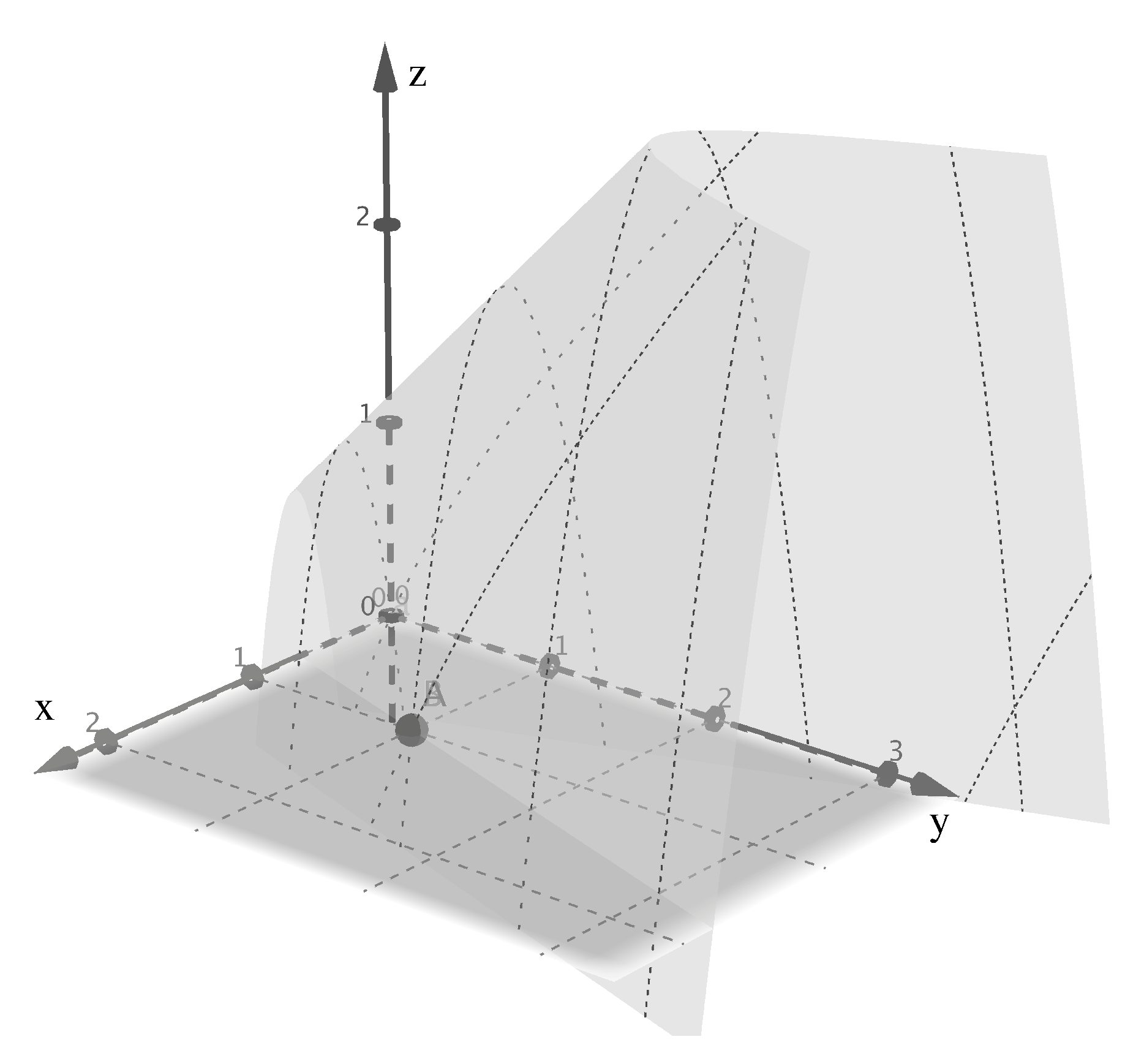
Example 10.

Consider $X=[-1,2]$ and $Y=[1,2]$. Let us evaluate $Z=Y-\frac{X·X}{Y}$. Using standard arithmetic (SIA) by few steps we reach $Z=[-3,4]$. By CIA:

$$Z=[\underset{\mathbf{0}\le {\lambda }_{\mathbf{x}},{\lambda }_{\mathbf{y}}\le \mathbf{1}}{\mathbf{min}}\theta ({\lambda }_x,{\lambda }_y),\underset{\mathbf{0}\le {\lambda }_{\mathbf{x}},{\lambda }_{\mathbf{y}}\le \mathbf{1}}{\mathbf{max}}\theta ({\lambda }_x,{\lambda }_y)],$$

(19)

and we need to optimize:

${\displaystyle \theta ({\lambda }_x,{\lambda }_y)=({\lambda }_y+1)-\frac{{(3{\lambda }_x-1)}^2}{({\lambda }_y+1)}}$on$[0,1]\times [0,1]$(see Figure 2).

Applying the gradient method, after many evaluations we find: $\mathbf{min}\mathit{\theta }=-3$ for ${\lambda }_x=1$ and ${\lambda }_y=0$, and $\mathbf{max}\mathit{\theta }=2$ for ${\lambda }_x=\frac{1}{3}$ and ${\lambda }_y=1$, hence $Z=[-3,2]$. The main difference concerns on $X\times X$, in SIA $X\times X\ne X^2$. But in CIA $X\times X=X^2$.

Note that CIA reduces overestimation comparing with SIA. Also, in CIA $X-X=0$, $X/X=1$ and $X(Y+Z)=XY+XZ$. However, these advantages have a cost, because many evaluations are required the by optimization process to find the final result.

At a glance CIA seems solve the problem of interval overestimation and has good algebraic properties, but CIA can become complex and slow if we increase the number of variables or add multiplications/divisions. For instance, consider $X,Y$ intervals and $Z=2X-4Y$, in this case to find Z it is necessary to optimize a function $\theta$ with two variables on $[0,1]\times [0,1]$, where $\theta$ is linear, i.e., a plane on three dimensional space. The optimization in this case is very simple, since $\theta$ is a continuous function on compact box $[0,1]\times [0,1]$ and its minimum and maximum occurs on the border of the box, also as $\theta$ is a plane on ${\mathbb{R}}^3$ the minimum and maximum occur on $(0,0),(0,1),(1,0)$ and $(1,1)$. In fact, if we consider Z an expression formed by the sum or difference of any finite set of variables, to evaluate Z with CIA we need to evaluate $\theta$ on $(0,0,\dots ,0),(1,0,\dots ,0),\dots (1,1,\dots ,1)$ and take the minimum and maximum.

However, if $Z=X·Y$ or $Z=\frac{X}{Y}$, the process can become complex, since the global minimum and maximum of $\theta$ can occur in the interior of the box (see Figure 2 from Example 10) and one needs to use the optimization process to find them. If we increase the number of variables, for instance $Z=XYK$, the optimization process becomes more complex. In this case, to find Z it is necessary to optimize $\theta$ on the hyper-rectangle $[0,1]\times [0,1]\times [0,1]$.

5. Final Remarks

This paper proposed a pair of axioms to characterize what would be a suitable interval division. The axiomatic system is inspired on what we call the partition principle (PP), which appears in different contexts. The most important application of this principle is on the process of data normalization. It is the starting point to answer the question:

“What would be a normalization of interval data?”

We think we have provided an answer for that by stating the axioms (D-1) and (D-2).

Axiom (D-2) states that the requirement to reflect the notion of normalization is that a suitable division should not introduce impreciseness. However, this axiom can be weakened in order to permit a controlled introduction of impreciseness, namely:

(D-2i)$\exists c>0,w\left(N\left(A\right)\right)\le c·{\displaystyle \sum _{j=1}^n}w\left(A_j\right)$, for all $1\le j\le n$.

This axiom generalizes (D-2), since (D-2) is the case for $c=1$. We have not found an interval division that satisfies it, however we proposed it here for future proposals of division.

Among the arithmetics investigated here, CIA is the only one that provides a division that captures the notion of normalization. As we have observed, it considers the whole expression to optimize it and recover the resulting interval. Since the space of functions is a distributive ring, it provides good algebraic properties for constrained intervals, however with the drawback of optimization, since a sequence of multiplications or division can become very hard to compute. Therefore, CIA cannot be considered a representation of any interval computation.

Hitherto, we have many proposals to represent intervals and operate with them. The idea is that the interval data could be translated to these representations, which will perform a computation in which the result will be transformed back to the usual interval representation. This is clear in approaches like: Hansen’s, AA and CIA.

Since just CIA captures the notion of normalization, it is the only thing (at least here) that must be applied to execute such a procedure during the computation of interval data. However, the optimization issues can forbid us to execute all the computation using CIA. Another point is that operations like sum and difference of different works are like the same operations in SIA, which is fast and simple. Hukuhara operations are other options in the scenario.

What we want to mean is that we can think of interval computation from another perspective, instead to operate with intervals by using a single representation we propose the computation of interval expressions by using different representations. In other words, sub-expressions of an interval expression are translated to a suitable representation (e.g., Affine, Hansen), its computation is performed and the resulting (converted back) interval replaces the sub-expression. Normalization is always made by using CIA.

One consequence is that this approach will lead us to review the role of intervals on fuzzy arithmetic and fuzzy algebra, since most of the proposals deal with $\alpha$-cuts [20].