New Modeling Approaches Based on Varimax Rotation of Functional Principal Components

Abstract

Functional Principal Component Analysis (FPCA) is an important dimension reduction technique to interpret the main modes of functional data variation in terms of a small set of uncorrelated variables. The principal components can not always be simply interpreted and rotation is one of the main solutions to improve the interpretation. In this paper, two new functional Varimax rotation approaches are introduced. They are based on the equivalence between FPCA of basis expansion of the sample curves and Principal Component Analysis (PCA) of a transformation of the matrix of basis coefficients. The first approach consists of a rotation of the eigenvectors that preserves the orthogonality between the eigenfunctions but the rotated principal component scores are not uncorrelated. The second approach is based on rotation of the loadings of the standardized principal component scores that provides uncorrelated rotated scores but non-orthogonal eigenfunctions. A simulation study and an application with data from the curves of infections by COVID-19 pandemic in Spain are developed to study the performance of these methods by comparing the results with other existing approaches.

1. Introduction

Nowadays, the great advancement of technology makes it common to have high-dimensional data associated with a large number of highly correlated variables. Functional data is a type of high-dimensional data in which a large number of observations of one or more variables are available at a continuous argument, usually time, on a sample of individuals. Therefore, a sample of functional data is a set of functions (curves, surfaces, etc.) that vary in a continuous argument such as time. Examples of data of this type are given in very diverse areas such as life sciences, environment, economics, chemometrics and electronic, among others. Functional Data Analysis (FDA) deals with the statistical modeling of this type of data. A detailed study of the main FDA methodologies as well as relevant applications and computational aspects are described in the books by [1,2,3,4,5].

The most common FDA technique is Functional Principal Component Analysis (FPCA) introduced by [6] as a generalization of the reduction dimension multivariate technique PCA to the case in which the data are functions instead of vectors. The first papers on this topic were framed in the theory of second order stochastic processes with the Karhunen–Loève (KL) expansion being the main tool. Thanks to this probabilistic result, the sample functions are reconstructed in terms of a small set of uncorrelated variables called principal components, whose interpretation allows to explain the main modes of variation in the functional data set. The theoretical aspects related with the properties, asymptotic theory and inference results of FPCA in the general framework of Hilbertian random functions were deeply studied in [7,8,9].

Most of the functional data can not be observed directly so that the latent stochastic process of interest must be reconstructed from discrete observations of each sample curve on a fixed or random time grid, which can be dense or sparse and different for the sample individuals. One usual form of reconstructing the functional form of sample curves is by an expansion in terms of basis functions such as Fourier, B-splines or wavelets [10,11,12,13,14,15]. The equivalence between FPCA of basis expansion of functional data and certain multivariate PCA in terms of the basis coefficients data matrix was studied in [8]. On the other hand, different Bayesian approaches to FPCA were considered in [16,17]. In addition, nonparametric methods to perform functional principal components analysis for the case of irregularly spaced longitudinal data (sparse) were developed [18,19].

The problem inherent to many applications is that interpreting the components is not always straightforward. It is known that the greatest contribution in the structure of a functional principal component is given by the process variables associated with the greatest values of the corresponding weight curve at certain time points [20]. In some cases the principal components are difficult to interpret because the estimated weight functions have a lot of variability and lack of smoothness. One way to solve this problem is based on penalizing the roughness of the weight functions. Several penalized FPCA approaches were developed to improve the estimation of the principal weight functions in the case of smooth curves observed with error [21,22,23]. In other cases, the first principal component explains a very high percentage of the total variance and is a straightforward average or size effect. These problems are usually solved by a rotation of the weight functions that simplifies the component structure and therefore makes the interpretation easier. The main drawback of rotation is that it is not able to retain the two crucial properties of FPCA: uncorrelatedness of the components and orthogonality of the weight functions. The most popular rotation method is Varimax [24]. This criterion has been extended to FPCA in two different way: the first one is based on Varimax rotation of the matrix of basis coefficients of the weight functions, and the other one is based on Varimax rotation of the matrix of values of the weight functions in a grid of equally spaced time points [1]. Varimax criterion could be unhelpful when data have a strong seasonal behaviour leading to a periodic structure as well as trends and isolated features in the weight curves. This is because Varimax rotation does not take into account the dependence structure in functional data at nearby time points. In order to solve this problem, a functional factor rotation based on canonical correlation was introduced in [25] as a means of extracting nearly-periodic directions in the data (principal periodic components). In this paper, two new approaches for rotation of FPCA are introduced. Both are based on the equivalence between FPCA and multivariate PCA of certain transformation of the matrix of basis coefficients of the sample curves [26]. On the one hand, Varimax rotation of the eigenvectors provides orthonormal rotated eigenfunctions but the associated principal components are not uncorrelated anymore. On the other hand, Varimax rotation of the loadings associated with the standardized principal components yields uncorrelated components with non-orthogonal eigenfunctions.

After this introduction, theoretical aspects related with the Varimax functional rotation are developed in Section 2. The behaviour of the proposed rotation methodologies is tested on a simulation study in Section 3, where the results are compared with other functional Varimax approaches previously developed in the literature. An application on COVID-19 infection curves is developed in Section 4. Finally, a detailed discussion of the results is given in Section 5.

2. Rotation in Functional Principal Component Analysis

Let us begin by a brief summary on Varimax rotation of multivariate PCA before introducing the functional Varimax rotation approaches.

2.1. Rotation in PCA

The rotation of principal components has its origin in the Factor Analysis (FA) whose goal is to find out the dependence structure among several variables by expressing them in terms of a small number of non-observable latent variables called factors. The aim of rotation of the matrix of factor loadings (multiplication by an orthogonal matrix R) is to facilitate the interpretation so that each factor is associated with a small block of observed variables. That means that the columns of the rotated loading matrix have high values for several variables and low for the remainder (the most elements either close to zero or far from zero, and with as few as possible values taking intermediate values). This approach gives raise to different criteria for defining the type of rotation which is designed to simplify the structure of loadings. Varimax, quartimax and promax are the most usual orthogonal methods meanwhile oblimax provides oblique factors by allowing R to be not necessarily orthogonal. The contributions of this paper are based on Varimax criterion which is the most applied in practice thanks to its good interpretation results. This type of rotation can be extended to PCA in order to simplify the structure of the problem and to facilitate the interpretation.

Formally, let X be a data matrix associated with a sample of size n of p random variables $(X_1,\cdots ,X_p).$ Let us suppose without loss of generality that the variables are centered. PCA can be applied by means of Singular Value Decomposition (SVD), that is, $X=UD{V}^T$ where U is a $(n\times p)$ unitary matrix, D is a $(p\times p)$ diagonal matrix whose principal diagonal is formed by the singular values and V is a $(p\times p)$ orthogonal matrix whose columns are the eigenvectors of the covariance matrix of X given by ${\Sigma }_{p\times p}=X^{T}X/(n-1)=V\Lambda V^T,$ with $\Lambda$ being a diagonal matrix whose elements are the eigenvalues of $\Sigma .$ Then, the following principal component representation is obtained:

$$X=UD\times V^T=Z{V}^T,$$

where $Z=UD$ are the principal components (PCs) scores and the columns of matrix V are also called principal directions or axes of the PCA. It is well known that the eigenvectors associated with different PCs are orthogonal ($V^{T}V=I$) and that all the p unrotated components are uncorrelated $Z^{T}Z/(n-1)=\Lambda .$ On the other hand, the standardized PC scores (uncorrelated scores with unit variance) denoted by $\tilde{Z}$ are given by $\tilde{Z}=Z{\Lambda }^{-1/2}=Z{D}^{-1}\sqrt{n-1}=U\sqrt{n-1},$ so that the data matrix is expressed as $X=\tilde{Z}{\Delta }^T,$ with $\Delta =VD/\sqrt{n-1}$ being the loadings associated with the standardized PCs which are eigenvectors scaled by the corresponding singular values.

There are two different ways to perform the rotation that provide different interpretation results. Thus, by considering the first $q<p$ p.c’s, X can be approximated by means of SVD as $X^q=U_q{D}_q{V}_q^T$ and the orthogonal rotation matrix R can be inserted through the following two possibilities:

• $X^q=\left(U_q{D}_{q}R\right)\left(R^T{V}_q^T\right)=Z_q^R{V^T}_q^R.$
• $X^q=\left(U_{q}R\right)\left(R^T{D}_q{V}_q^T\right)={\tilde{Z}}_q^R{{\Delta }^T}_q^R.$

One is based on rotating the loadings of PCs (eigenvectors) and the other in rotating the loadings of the standardized PCs (eigenvectors scaled by the singular values). In the first option the new scores provided by the rotation will not be uncorrelated anymore although the axes do will remain orthogonal. This is not how PCA is usually understood and applied. For that reason, it is quite common not to call them anymore rotated PCs but only rotated components. By contrast, in the second option the rotated loadings are not orthogonal axes but the rotated scores continue to be uncorrelated. Any of these approaches can be considered but in order to interpret the results it is important to take these properties into account. In fact, and according to our research, even the experts in this field do not reach an agreement about what method is better or what approach must be considered more often in practice. Therefore, it seems reasonable to conclude that there is not an ideal method for rotating the PCs and any of them can be employed. Another important aspect has to do with the amount of variance explained by the rotated components. After applying the Varimax rotation, the variance explained by the first q components remains unchanged and gets redistributed among the rotated components so that the quantities are not arranged in descending order.

Let us remember that in Varimax rotation the matrix R is computed by maximizing the variance of the coefficients that define the effect of each factor on the observed variables. Then, in PCA R is chosen to maximize the variability of the squares elements of the rotated matrix of eigenvectors/loadings. In any case, the amount of explained variance by each rotated component is determined by the following formula:

$$V{T}_k^R=\frac{{\delta }_k}{{\sum }_{k=1}^q{\delta }_k}\times V{T}_q,$$

where ${\delta }_k$ is the kth value of the diagonal of ${Z^R}^T{Z}^R$ and $V{T}_q$ is the proportion of total variance captured by the first q PCs. Let us observe that the criterion of rotating the loadings provides the same proportion of variance explains by each one of the rotated standardized components. This fact is due to the properties of the matrix U from the SVD analysis.

2.2. Rotation in Functional PCA

For many reasons, FPCA is the basic tool in FDA. It is an extension of PCA which is crucial to reduce the infinite dimension of functional data and to explain the variability and dependence structure of functional variables in terms of a reduce set of uncorrelated variables called functional PCs [6].

Let $\{x_i\left(t\right):t\in T,i=1,\dots ,n\}$ be a size n sample of curves associated with a second order and quadratic mean functional variable X defined on a probabilistic space $(\Omega ,\mathcal{A},P),$ whose sample curves belong to the space $L^2\left(T\right)$ of square integrable functions on a real interval T, with the natural inner product defined as

$$〈f,g〉={\int }_{T}f\left(t\right)g\left(t\right)dt,\forall f,g\in L^2\left[T\right].$$

Let us also assume without loss of generality that the functional variable X is centered.

The principal components are uncorrelated generalized linear combinations with maximum variance (Var). In general, the j-th principal component score is given by

$$z_{ij}={\int }_T{x}_i\left(t\right)f_j\left(t\right)dt,i=1,\dots ,n,$$

where the weight function (loading) $f_j$ is obtained by maximizing the variance

$$\left\{\begin{array}{cc}Ma{x}_{f}Var\left[{\int }_T{x}_i\left(t\right)f\left(t\right)dt\right]\hfill & \\ {r.t.\parallel f\parallel }^2=1\mathrm{and}\int f_{\ell }\left(t\right)f\left(t\right)dt=0,\ell =1,\dots ,j-1.\hfill \end{array}\right.$$

This problem is solved in term of the eigenanalysis of the sample covariance operator $C.$ That is, the solutions to the second order integral equation

$$C\left(f_j\right)\left(t\right)=\int c\left(t,s\right)f_j\left(s\right)ds={\lambda }_j{f}_j\left(t\right),$$

where $c\left(t,s\right)$ is the sample covariance function and ${\lambda }_j=Var\left[z_j\right].$ Then, the following principal component decomposition of the sample curves is obtained: $x_i\left(t\right)={\sum }_{i=1}^{n-1}{z}_{ij}{f}_j\left(t\right),$ that can be truncated in the $qth$ term providing the best least squares linear approximation of the sample curves $x_i^q\left(t\right)={\sum }_{i=1}^q{z}_{ij}{f}_j\left(t\right),$ with explained variance given by ${\sum }_{i=1}^q{\lambda }_i.$ The most usual criterion for choosing the number of PCs consist of selecting the first q components whose proportion of explained variance is close to one (at least 0.75–0.8 in most cases).

In order to estimate the eigenvalues and eigenvectors, it is usual to assume that sample paths belong to a finite-dimension space generated by a basis $\{{\varphi }_1\left(t\right),\dots ,{\varphi }_p\left(t\right)\}$, so they can be expressed as

$$x_i\left(t\right)=\sum _{j=1}^p{a}_{ij}{\varphi }_j\left(t\right)=a_i^{\prime }\mathsf{\Phi }\left(t\right),i=1,\dots ,n,$$

where p must be sufficiently large to get an accurate representation of the curves. The selection of the type and dimension of the basis is a crucial problem that must be solved by keeping in mind the characteristics of the curves. Normally, Fourier basis is used when the curves are periodic, B-spline basis is employed for non-periodic smooth paths and wavelet basis for data with a strong local behaviour. Once the basis is selected, the basis coefficients are commonly approximated by least squares from noisy discrete time observations of each sample curve.

In this context, FPCA is equivalent to multivariate PCA of matrix $A{\mathsf{\Psi }}^{1/2}$, with $A={\left(a_{ij}\right)}_{n\times p}$ being the matrix of basis coefficients and ${\mathsf{\Psi }}^{1/2}$ being the squared root of the matrix of inner products between basis functions $\mathsf{\Psi }={\left({\mathsf{\Psi }}_{ij}\right)}_{p\times p}={\int }_T{\varphi }_i\left(t\right){\varphi }_j\left(t\right)dt,i,j=1,\dots ,p$ [26]. Then, the PC weight functions admit the following basis expansion:

$$f_j\left(t\right)=\sum _{k=1}^p{b}_{jk}{\varphi }_k\left(t\right),$$

where the vector $b_j$ of basis coefficients is given $b_j={\mathsf{\Psi }}^{-1/2}{v}_j$ where the $v_j$ are computed as the eigenvectors of the sample covariance matrix of $A{\mathsf{\Psi }}^{1/2}.$ Then, $Z={\left(z_{ij}\right)}_{n\times p}=\left(A{\mathsf{\Psi }}^{1/2}\right)V$ is the matrix whose columns are the PC scores of $A{\mathsf{\Psi }}^{1/2}$ and V the one whose columns are its associated eigenvectors. In matrix form, the basis expansion of weight functions would be $f=B^T\mathsf{\Phi },$ with $f={(f_1,\cdots ,f_p)}^T$ being the vector with the eigenfunctions, B the matrix of basis coefficients $B_{p\times p}=\left(b_{ij}\right)={\mathsf{\Psi }}_{p\times p}^{-1/2}{V}_{p\times p},$V the matrix with columns the eigenvectors of the covariace matrix of $A_{n\times p}{\mathsf{\Psi }}_{p\times p}^{1/2},$ and $\mathsf{\Phi }={({\varphi }_1,\dots ,{\varphi }_p)}^T,$ the vector of basis functions.

Functional Varimax Rotation

Two different ways of functional varimax rotation were proposed so far [1]. One is based on rotating the matrix of basic coefficients of the eigenfunctions and the other, coarser, on rotating the matrix of values of the eigenfunctions in a grid of equally spaced time points. In both cases the rotated component scores are no longer uncorrelated although the weight functions (axes) after rotation are still orthonormal. At this point, the new methodology that we propose for rotating the functional PCs consists of rotating PCA of the matrix $A{\mathsf{\Psi }}^{1/2}$, based on the statement that FPCA is equivalent to multivariate PCA of this matrix. This is the main contribution of the current study in addition to doing an exhaustive revision about different ways of functional Varimax rotation and a comparison study among them. As a natural extension of the multivariate case, our proposal considers two different possibilities depending whether the rotation is done on the eigenvectors or on the loadings of the standardized principal component scores. This way, the rotation of the functional principal components is inspired by the theory of rotation of factor analysis presented in previous subsection by considering the multivariate viewpoint in the FDA context.

More formally, FPCA rotation would consists of rotating the first q PC weight functions as $f_q^{R^T}=f_q^{T}R.$ This way, the vector $n\times 1$ with the sample functions is approximated in terms of the first q PCs as

$$X^q=Z_q{f}_q=\left(Z_{q}R\right)\left(R^T{f}_q\right)=Z_q^R{f}_q^R,$$

where the vector of rotated eigenfunctions is expressed as $f_q^{R^T}={\mathsf{\Phi }}^T{B}_{q}R={\mathsf{\Phi }}^T\left({\mathsf{\Psi }}^{-1/2}{V}_q\right)R$ with $B_q$ being the matrix of basic coefficients associated with the first q eigenfunctions and $V_q$ the matrix whose columns are the first q eigenvectors. This expression was our inspiration to propose a methodology based on directly rotating the eigenvectors instead of the methodology based on rotating the basic coefficients proposed by [1].

Thus, the chances in order to rotate functional PCA are the following:

R1

Applying the VARIMAX rotation criterion to weight function values.

In this case, the purpose would be to find a matrix R that maximizes the variance of the squares of the elements of the matrix

$$F_q^{R^T}=F_q^{T}R,$$

where $F_q$ is the $q\times m$ matrix whose elements are the values of the first q eigenfunctions evaluated at a grid of time points $t_1,\dots ,t_m,$ given by $F_q^T={\mathsf{\Gamma }}^T{\mathsf{\Psi }}^{-1/2}{V}_q,$ with $\mathsf{\Gamma }$ being the $p\times m$ matrix that contains as rows the values of each basis function at the time points.

R2

Applying the VARIMAX rotation criterion to weight function coefficients.

In this occasion, the goal is to calculate a matrix R that maximizes the variability of the squares elements of $B^R=BR={\mathsf{\Psi }}^{-1/2}VR.$ Then, the rotated principal factors are given by

$$f_q^{R^T}={\varphi }^T{B}^R.$$

R3

Applying the VARIMAX rotation criterion to PCs by rotating the matrix of eigenvectors.

Here, the objective is to determine a matrix R that maximizes the variability of the squares elements of the rotated matrix of eigenvectors $V_q^R=V_{q}R.$ Then, the rotated principal factors are given by

$$f_q^{R^T}={\varphi }^T\left({\mathsf{\Psi }}^{-1/2}{V}^R\right).$$

R4

Applying the VARIMAX rotation criterion to the standardized PCs by rotating the matrix of loadings

Hence, this method consists of computing a matrix R that maximizes the variance of the squares elements of the matrix ${\Delta }_q^R={\Delta }_{q}R=V_q{\Lambda }_q^{1/2}R.$ Then, the rotated principal factors are given by

$$f_q^{R^T}={\varphi }^T\left({\mathsf{\Psi }}^{-1/2}{\Delta }_q^R{\Lambda }_q^{-1/2}\right).$$

The two last functional Varimax approaches (R3 and R4) are the main contribution of this paper based on Varimax rotation of the multivariate PCA of $A{\mathsf{\Psi }}^{1/2}$ matrix, which is equivalent to functional PCA of $X.$ On the other hand, methods R1 and R2 are not new and are considered in this paper only for comparison purpose in the simulation study. Let us observe that in the case of orthonormal basis functions, approaches R2 and R3 match. Moreover, with the first three methods the rotated factors are ortonormal but the rotated components are not uncorrelated, meanwhile with the last one the opposite happens.

3. Simulation Study

The good performance of the two functional Varimax approaches introduced in this paper (R3 and R4) is tested on simulated data. The results will be compared with the ones provided by approaches R1 and R2 discussed in the book by [1].

The data are simulated from the approximation of the Wiener process (Brownian motion) given by its Karhunen–Loève (KL) expansion truncated in the q$th$ term. This is a Gaussian process with covariance function given by $C(t,s)={\sigma }^{2}min(t,s).$ The KL expansion of this process is given as follows in terms of the eigenvalues and eigenfunctions of the covariance operator:

$$X\left(t\right)=\sum _{k=1}^{\infty }\sqrt{{\lambda }_k}{\xi }_k{f}_k\left(t\right),$$

(1)

where the PCs ${\xi }_k$ are independent Gaussian random variables with mean zero and variance one, the eigenvalues are given by ${\lambda }_k=\frac{{\sigma }^2}{{(k-0.5)}^2{\pi }^2}$ and the eigenfunctions by $f_k\left(t\right)=\sqrt{2}\sin \left((k-0.5)\pi t\right)$. In this study, the cut-off $q=8$ and a dispersion parameter $\sigma =0.2$ were considered. Then, 500 samples of 150 sample curves of the process $X\left(t\right)$ given by Equation (1) were simulated at different number of equally spaced knots in the observed domain [0, 1]. Three different scenarios were considered by defining the time points as $t_k=k/m,k=0,1,\cdots ,m;m=25,50,100.$ Different sample sizes were also considered but the results are not included in the paper because they were quite similar for sample sizes large enough.

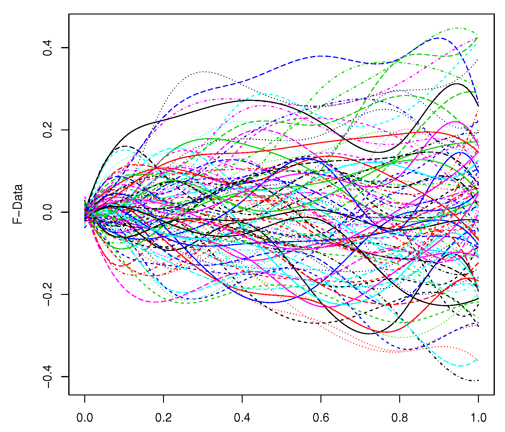
First, least squares approximation of each sample curve was performed in terms of a basis of cubic B-splines of dimension 8. The sample curves of one of the simulated samples are displayed in Figure 1. Then, functional PCA and the four considered functional Varimax approaches for rotating the first four components were performed.

Table 1. Percentages of variance explained by the first four PCs and their redistribution after the three types of Varimax rotation of the eigenfunctions.

PC	FPCA	R1	R2	R3
1	80.4	23.2	22.0	23.5
2	10.8	11.6	49.5	9.3
3	4.5	24.9	7.6	44.2
4	2.2	38.2	18.8	20.9

shows an example of the amount of variance explained by the first four PCs and the redistribution of the variances after applying the three type of rotation of the eigenfunctions aforementioned. Let us observe that the criterion of rotating the loadings (R4) is not included in this table because the same proportion of variance is distributed among the rotated standardized components $(24.48\%).$ This fact is due to the properties of the matrix U from the SVD analysis.

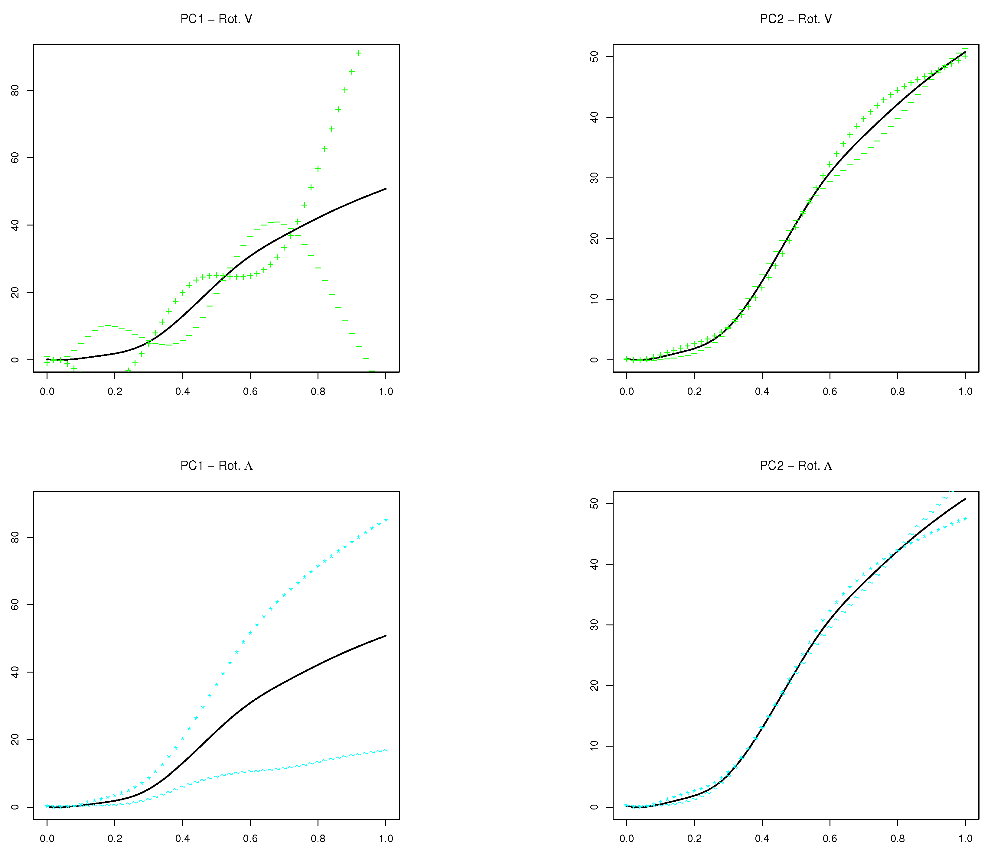
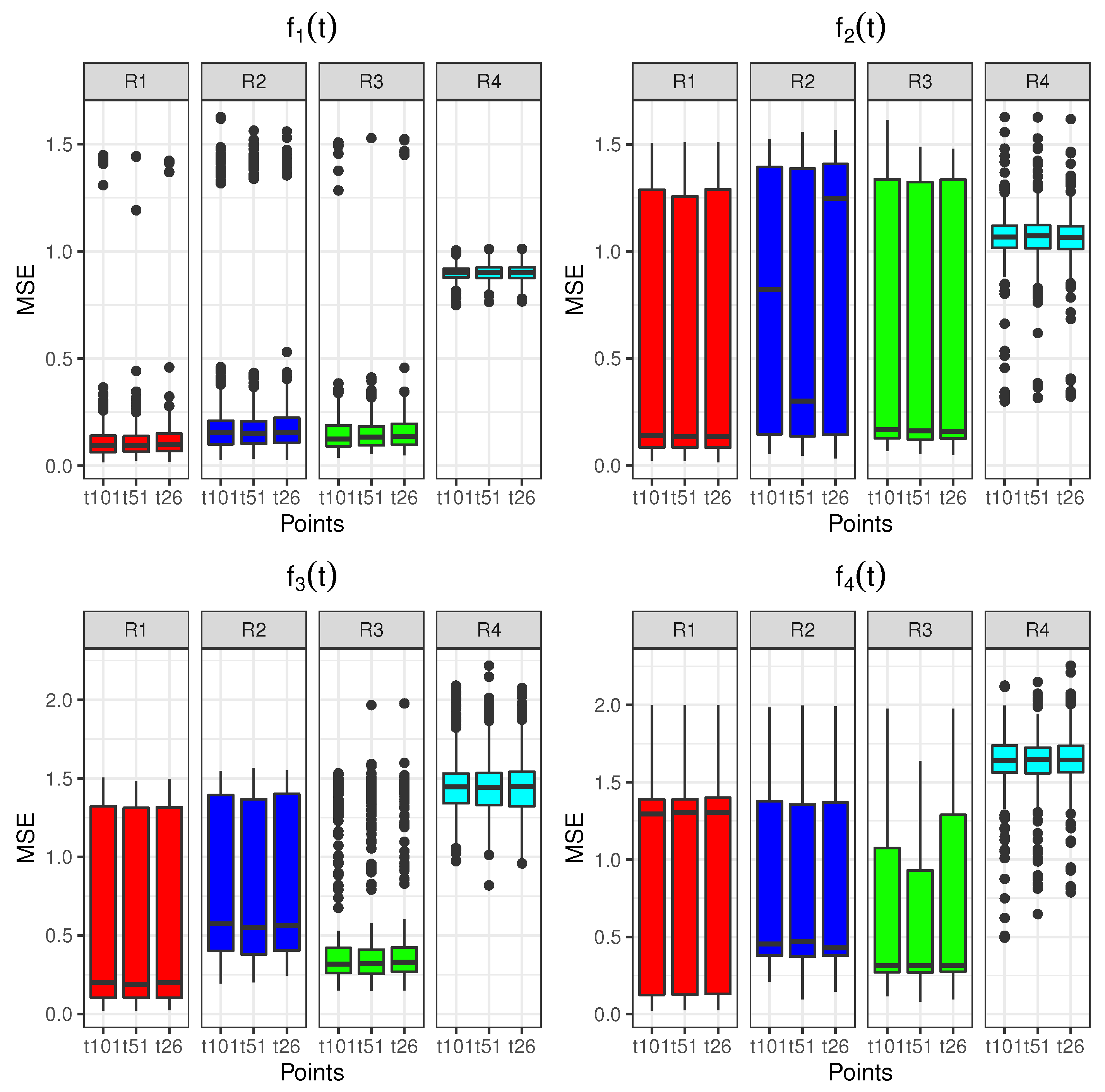
In Figure 2, the estimated eigenfunctions (FPCA) and their functional Varimax rotations by the four considered approaches (R1, R2, R3 and R4) are displayed for one of the simulated samples next to the original rotation of the theoretic values for the first four eigenfunctions. Theoretically, the rotated eigenfunctions with the first three approaches should resemble their corresponding original rotation. In order to draw general conclusions, the integrated mean squares error (MSE) of each rotated eigenfunction with respect to the original rotation is computed as the squared root of

$$\parallel f_i^R-{\widehat{f}}_i^R{\parallel }^2={\int }_T{\left[f_i^R\left(t\right)-{\widehat{f}}_i^R\left(t\right)\right]}^{2}dt={\int }_T{\left[\sum _{j=1}^p{d}_{ij}{\varphi }_j\left(t\right)\right]}^{2}dt=d_i^{\prime }\mathsf{\Psi }{d}_i,$$

where $d_i={\left(d_{i1},\dots ,d_{ip}\right)}^{\prime }$ is the vector with the differences between the basis coefficients of each original rotated eigenfunction and the ones of its estimation by using the different type of functional rotations. The boxplots of the MSEs for the rotated eigenfunctions estimated by using R1, R2 and R3 with 26, 51 and 101 observed time points for 500 simulations of the Wiener process were plotted in Figure 3. Rotation R4 is included in these boxplots although the estimated eigenfunctions are not orthogonal and the comparison with the other approaches makes no sense. Let us observe that the new Varimax rotation of the eigenfunctions introduced in this paper (R3) provides the most accurate results, which are also more robust with respect to the number of observation nodes of the sample curves.

4. COVID-19 Data

In order to show up the usefulness of rotation to facilitate the interpretation of the principal components, an application with data from COVID-19 pandemic has been developed. The functional data are the number of daily cumulative informed cases of COVID-19 for seventeen autonomous communities (ACs) in Spain from 20/02/2020 to 27/04/2020 (first wave of COVID-19). Data source: https://cnecovid.isciii.es/covid19/#documentación-y-datos. The sample curves, denoted by $x_1\left(t\right),\dots ,x_{17}\left(t\right),$ are daily observed starting the day that at least one case is reported. Therefore, the period of observation and the number of observations are different for each AC. In order to homogenize the data, the number of cases per 10,000 inhabitants is considered and the first observation for each curve corresponds to the day that exceeds by first time the maximum of the first reported values. Then, all the curves were registered in the common interval [0, 1]. A detailed description of basis approaches for functional data registration can be seen in [1].

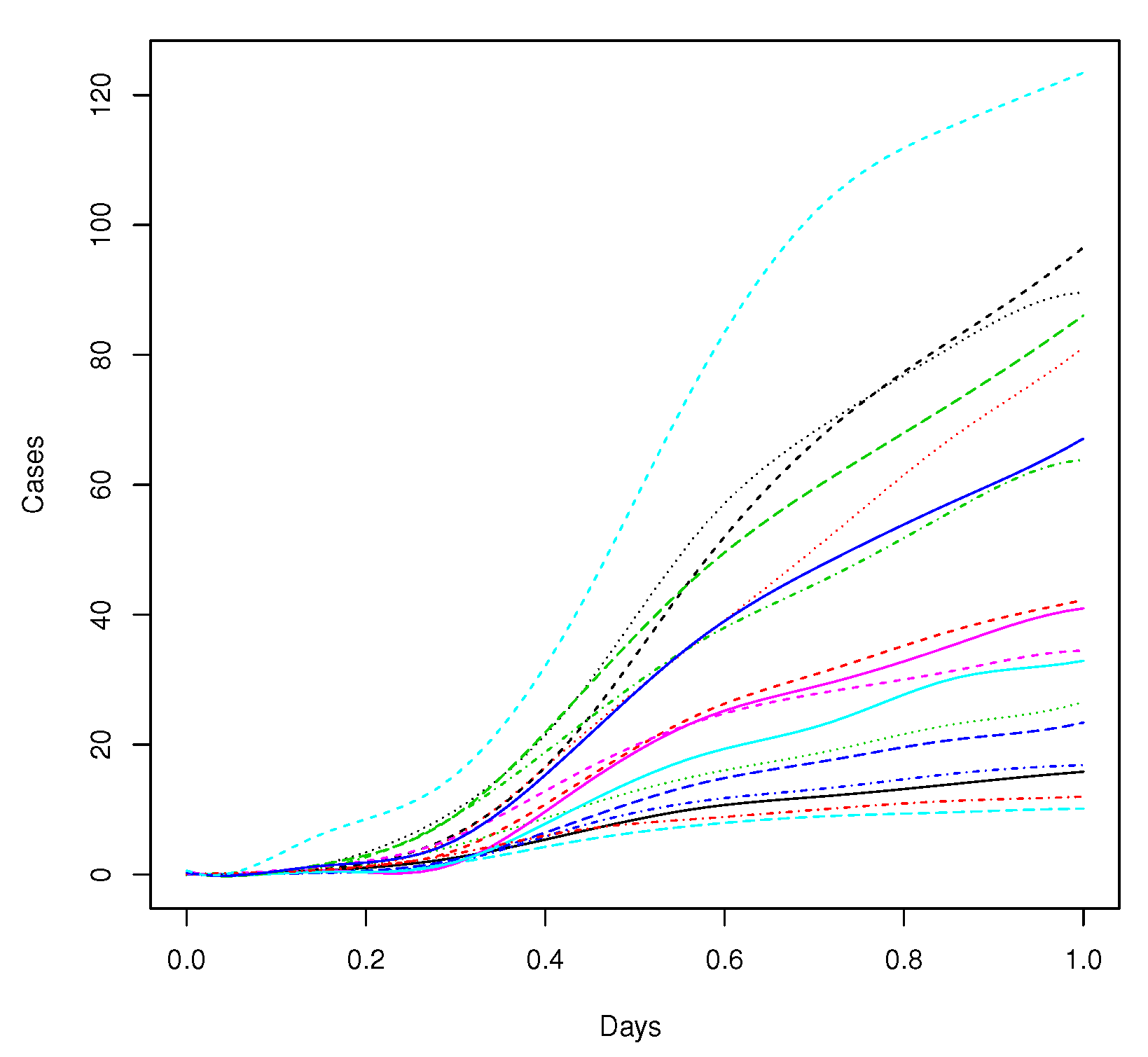
The first step for estimating FPCA is to approximate the sample curves in terms of an appropriate functional basis by using least squares smoothing. A B-spline basis of dimension 10 with equally spaced knots in the interval [0, 1] was chosen in this paper for the functional representation of each curve. Figure 4 shows all the smoothed sample curves.

Second, FPCA was performed in order to reduce the dimension of the problem and to explain the different modes of variability in the data. As the first principal component explains more than 99% of the total variability the results are not easy to interpret (

Table 2. Percentages of variance explained by the first four PCs of COVID-19 data per 10,000 inhabitants for seventeen autonomous communities in Spain.

PC	FPCA	Rotation R3
1	99.32	44.36
2	0.52	38.14
3	0.12	0.67
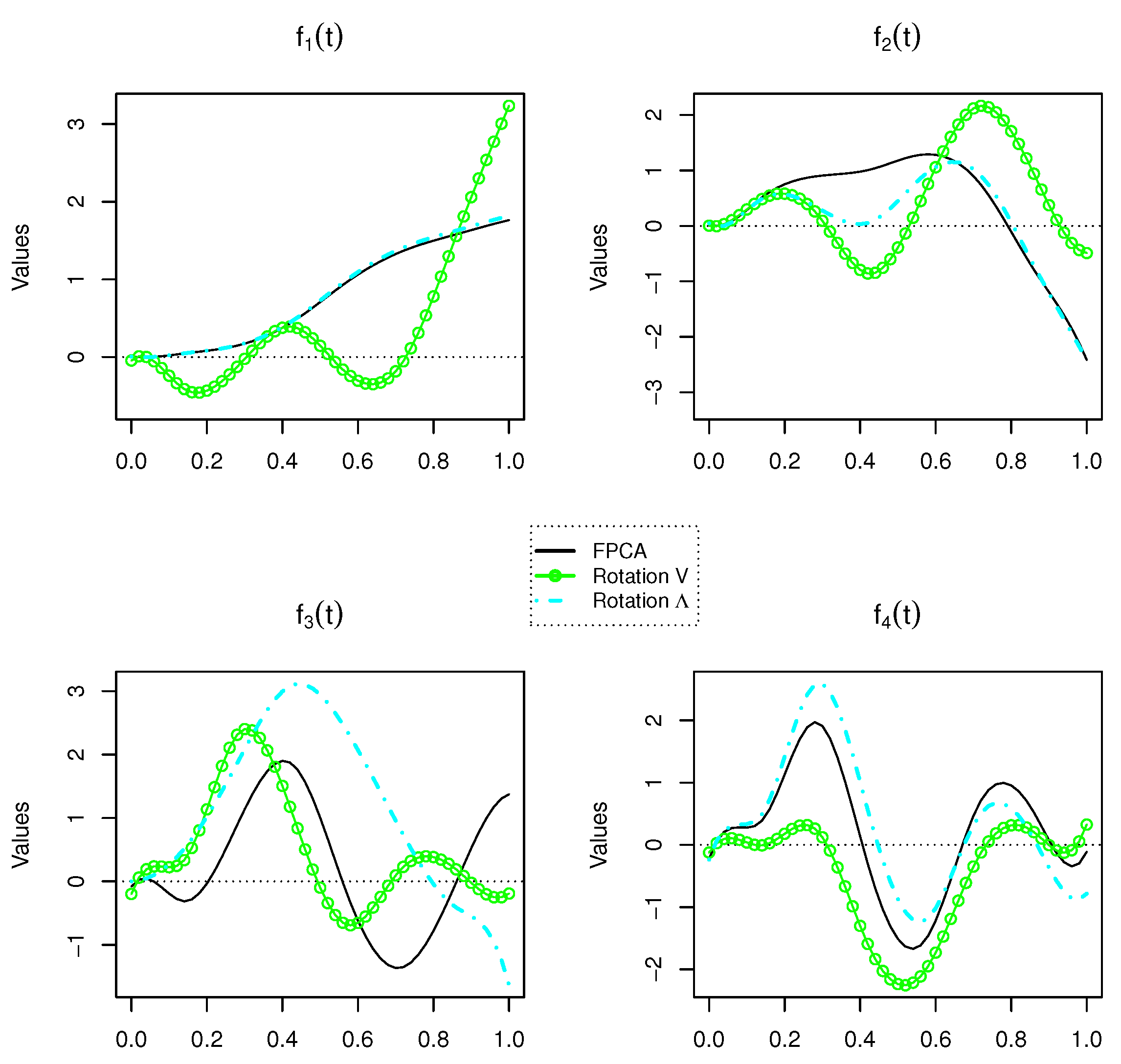
4	0.03	14.82

). The estimated first four weight functions are displayed in Figure 5 (black line). Let us observe that the first eigenfunction is positive and strictly increasing through the entire observation period, and in addition, the weight placed on the cases at the end is about two times higher than at the beginning. This could lead to interpret that the most important mode of variation between ACs represents a quick increase in cases as time passed with the infection curve out of control. The rest of the components are difficult to interpret since they account for much smaller and insignificant proportions of the total variation.

Third, in order to obtain weight functions and PC scores much easier to interpret, the two Varimax rotation approaches introduced in this paper (R3 and R4) are carried out on the first four PCs. This way, the variability explained by the first four rotated components is divided in different proportions, which can be seen in Table 2. Let us now observe that the first two rotated components explain more than a $82\%$ of the total variability with the main mode of variation accounting a $44\%$ and the second a $38\%$ approximately. The first four rotated eigenfuntions are shown in Figure 5. Taking into account their explained variances, only the first two rotated components will be interpreted. The first two eigenfunctions plotted as positive and negative perturbations of the mean function are shown in Figure 6 with the first row corresponding to the rotation of eigenvectors (R3) and the second one to the rotation of loadings (R4 approach). The scores of the seventeen Spanish ACs on the first two rotated principal components of COVID-19 cases are displayed in Figure 7 for R3 (left) and R4 (right) rotation approaches, where the location of each AC is shown by the abbreviation of its name assigned in

Table 3. Abbreviation of the seventeen Spanish autonomous communities.

Andalucía, AN	Castilla-La Mancha, CM	Madrid, MD
Aragón, AR	Castilla-León, CL	Murcia, MC
Asturias, AS	Cataluña, CT	Navarra, NC
Islas Baleares, IB	Comunidad Valenciana, VC	País Vasco, PV
Canarias, CN	Extremadura, EX	Rioja, RI
Cantabria, CB	Galicia, GA

.

Let us begin by interpreting the results given by R3 approach (rotation of eigenvectors). Now, the first eigenfunction is easier to interpret and represents those ACs that had an increase more or less constant until the $70\%$ of the observed period where the number of cases shot up leaving the curve out of control. The three highest scores are assigned to La Rioja (RI), Madrid (MD) and Castilla la Mancha (CM), which were the communities with more problems controlling the infections and the largest negative scores to Canarias (CN), Murcia (MC) and Andalucía (AN), which were the communities that better controlled the infection curve. On the other hand, the behaviour of the second eigefunction represents those ACs which suffered an increase relatively rapid between the 40% and 70% of the period but they managed to have the curve under control from that moment.

Regarding R4 approach (rotation of loadings), the behaviour of the first and second eigenfunctions is very similar to the unrotated ones. That is, the first is associated with those ACs that did not control the curve because as the days passed, the number of cases increased very quickly. On the other hand, the second eigenfunction could be influenced by the ACs which controlled the number of cases since the time representing the $60\%$ of the observed period. These conclusions are corroborated by Figure 5 and Figure 6. Les us observe from Figure 7 (left) the high correlation between the first two rotated PCs scores provided by approach R3 that establishes two clearly differentiated groups between the autonomous communities: those ACs which managed to control moderately the curve of number of cases (third quadrant) and the ones that lost control of the cases by reaching numbers really concerning (first quadrant). On the other hand, thanks to the uncorrelation between the rotated PCs scores, approach R4 provides a much better clustering of AC. This can be seen in the biplot on the right in Figure 7 where each of these two groups is divided in other two so that four groups can be clearly distinguished.

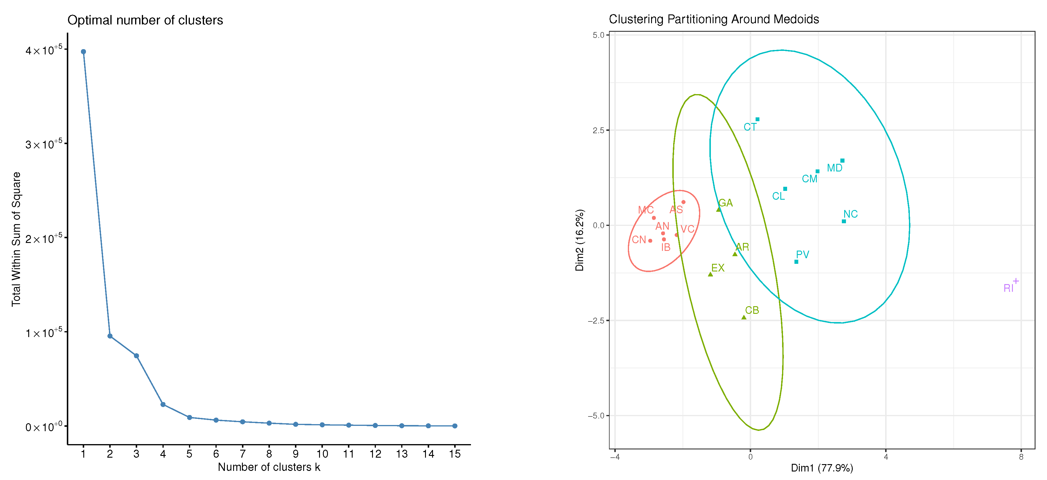
In fact, these conclusions agree with the results obtained after applying functional data clustering [27]. In particular, it has been considered the approach based on performing clustering using the basis expansion coefficients in terms of the basis of cubic B-splines aforementioned. Due to the fact that La Rioja (RI) could be an outlier, the K-medoids method, which is more robust than K-means, is applied next to Manhattan distance as similitude measure. Moreover, as the dataset is not too large, the algorithm called Partitioning Around Medoids is considered. In order to identify the optimum number of clusters, the reduction of intra-cluster total variance was evaluated for a range of values K (elbow method). It can be seen in the left panel of Figure 8 that the reduction seems to stabilize by starting at 4 cluster. Finally, the clustering results appear in the right panel of Figure 8 which is very similar to the biplot in the right panel of Figure 7. This is in accordance with multiple studies about the infections by COVID-19 pandemic in Spain [28,29,30,31], what corroborate the good interpretation and classification results provided by the new rotation approaches introduced in this paper.

5. Discussion

FDA try to solve problems where the involved sample data are functions that vary over some continuum, usually time. One of the most important techniques in the field of FDA is Functional Principal Component Analysis, whose main purpose is to reduce the dimension of the problem and to explain the dependence structure of data in terms of a reduce set of uncorrelated variables called functional principal components. The interpretation of these components helps to understand the main characteristics and modes of variation of the underline stochastic process. Nevertheless, there are many situations in which this task is not easy. One is the case when the first PC represents a size effect that explains a very high percent of the total variability. The most common tool to solve this problem in PCA is Varimax rotation that redistributes the explained variance among all rotated components to make easier the interpretation. So far, there were only two approaches available in the literature to apply Varimax rotation in the FDA context, but neither of them is a direct rotation of eigenfunctions. The first one consists of rotating the values of the weight functions evaluated at the time points (R1), while the second one is based on rotating the weight function coefficients (R2). Both methods retain the orthogonality of the axis but the new scores will not be uncorrelated anymore. In this paper, two new approaches based on the equivalence between FPCA of basis expansion of the sample curves and PCA of a transformation of the matrix of basis coefficients are proposed: one is based on applying the Varimax criterion to principal components by rotating the matrix of eigenvectors (R3), and the other makes use of the Varimax criterion on the standardized principal components by rotating the matrix of loadings (R4). The first one guarantees the orthogonality of the rotated eigenfunctions and in the second one the rotated scores are still uncorrelated. Moreover, all of them are compared in an exhaustive simulation study. From this study it can be concluded that R3 provides the most accurate rotated eigenfunctions and is also more robust with respect to the number of discrete time observations of the sample curves. Finally, an application with the curves of infections by COVID-19 pandemic in Spain has been developed. Through the combination of these two new varimax approaches (R3 and R4), it has been possible to distinguish different behaviors in the evolution of infections in the Spanish autonomous communities during the first wave of the pandemic. These results are in agreement with other studies done in the country about this matter [28,29,30,31]. These Varimax FPCA approaches are expected to be welcomed and highly employed in future researches in different areas of science thanks to their ability to facilitate the interpretation of the main patterns of variation in the data.