A Note on the Asymptotic Normality Theory of the Least Squares Estimates in Multivariate HAR-RV Models

Abstract

In this work, multivariate heterogeneous autoregressive-realized volatility (HAR-RV) models are discussed with their least squares estimations. We consider multivariate HAR models of order p with q multiple assets to explore the relationships between two or more assets’ volatility. The strictly stationary solution of the HAR($p,q$) model is investigated as well as the asymptotic normality theories of the least squares estimates are established in the cases of i.i.d. and correlated errors. In addition, an exponentially weighted multivariate HAR model with a common decay rate on the coefficients is discussed together with the common rate estimation. A Monte Carlo simulation is conducted to validate the estimations: sample mean and standard error of the estimates as well as empirical coverage and average length of confidence intervals are calculated. Lastly, real data of volatility of Gold spot price and S&P index are applied to the model and it is shown that the bivariate HAR model fitted by selected optimal lags and estimated coefficients is well matched with the volatility of the financial data.

1. Introduction

Volatility in financial asset returns is one of the most important components in the financial market for optimization decisions such as portfolio selection, risk management and asset pricing. Over recent decades, extensive research works by statisticians and econometricians have analyzed volatility alongside time series modelings. In particular, because multiple assets are correlated with each other in the financial markets, the cross-correlation of two or more asset returns and the spillover effect of the volatility have been represented in multivariate time series models rather than the univariate models. Probabilistic properties such as long-memory of the volatility, which means that historical volatility has a persistent impact on future volatility, have been imposed efficiently to time series models through various statistical techniques.

In order to capture the long-memory persistence of the volatility, Corsi [1] suggested a simple but remarkably efficient time series model with additive cascades defined on different time periods by incorporating the daily, weekly and monthly volatility components. Corsi’s model [1] called a heterogeneous autoregressive-realized volatility model of order 3, (HAR-RV(3) or simply HAR(3)), is a type of linear autoregression with heterogeneous regressors, which are previous lag, lagged weekly moving average, and lagged monthly moving average. Since its introduction, various adaptive versions of the HAR model are used to analyze the volatility along with empirical data analysis. Here, we refer to [2,3,4,5] for univariate data and [6,7,8,9,10,11] for multivariate data.

In particular, Bubak et al. [6] used a multivariate extension of the HAR model to uncover volatility transmission between Central European currencies and the EUR/USA foreign exchange rate, whereas Soucek and Todorova [8] employ a bivariate HAR model to explore the relationship between equity and oil market volatility. Cubadda et al. [9] proposed a vector HAR index model for detecting the presence of co-movements and analyzing the joint behavior in a set of daily realized volatility measures. Cech and Barunik [10] proposed a generalized HAR model for dynamic covariance matrix modelling and forecasting.

All of the references above empirically only dealt with the multivariate HAR models, but they have not presented theoretical results of the HAR model. Indeed, there is only a few of theoretical analysis of the HAR model, even in the univariate case. Furthermore, the least squares estimate (LSE) method has been popularly used as a tool of estimation in time series data analysis. The LSEs are used often in the literature to analyze the multivariate data in the multivariate HAR models and good performances on the volatility forecasting are obtained with forecast accuracy, for instance, see [9,12]. However, in the multivariate HAR models, rigorous formulation of asymptotic multivariate normality theory of the LSE has not yet been established in spite of the frequent uses of the LSEs. The earlier studies motivate us to consider multivariate HAR models of order p with q multiple assets, and look into theoretical analysis of the LSEs. In this work we provide, as a main result, strictly stationarity of the HAR($p,q$) model and asymptotic normality theories of LSEs for the parameters in the multivariate HAR models. The multivariate normalities of the LSEs are established in two cases of i.i.d. and correlated errors of the models. In addition, we consider an exponentially weighted multivariate HAR model and discuss the estimation of a common decay rate on coefficients in the exponentially weighted HAR model.

A Monte Carlo experiment is conducted to illustrate performance of the estimations. Sample mean and standard error of the LSEs as well as empirical coverage and average length of confidence intervals are calculated. In addition, we model volatility of Gold spot price and S&P500 index using a bivariate HAR model and estimate the coefficient parameters. The parameter estimates and confidence intervals are computed according to the asymptotic normality we derived. Finally, the bivariate HAR fitting is demonstrated to the market data with optimally selected lags under some criterion rules.

The remainder of the paper is organized as follows: In Section 2, the multivariate HAR model is presented with discussion on strictly stationary solution and in Section 3 the LSEs and their multivariate normalities are derived. Section 4 deals with the exponentially weighted multivariate HAR model. A Monte-Carlo experiment is performed and an application with market data is given in Section 5 and Section 6, respectively. We conclude in Section 7, where the main conclusion and discussion on future works are stated.

2. Multivariate HAR($\mathit{p}\mathbf{,}\mathit{q}$) Models

We consider the following HAR-RV model $\{Y_{1,t}:t\in \mathbb{Z}\}$ with multivariate data $\{Y_{j,t}:t\in \mathbb{Z},j=2,\dots ,q\}$ which has been discussed in [8] as an extension of the HAR-RV(3) model in [1].

$$Y_{1,t}\equiv Y_{1,t}^{\left(d\right)}={\beta }_0+\sum _{i=d,w,m}{\beta }_1^{\left(i\right)}{Y}_{1,t-1}^{\left(i\right)}+\sum _{i=d,w,m}{\beta }_2^{\left(i\right)}{Y}_{2,t-1}^{\left(i\right)}+\cdots +\sum _{i=d,w,m}{\beta }_q^{\left(i\right)}{Y}_{q,t-1}^{\left(i\right)}+{ϵ}_{1,t}$$

(1)

where $\{{ϵ}_{1,t},t\in \mathbb{Z}\}$ are random variables for error terms and $\{{\beta }_0,{\beta }_j^{\left(i\right)},j=1,\dots ,q;i=1,\dots ,p\}$ are coefficient parameters. For each jth-asset, $j=1,2,\dots ,q$, three volatility components $Y_{j,t-1}^{\left(i\right)}$, $i=d,w,m,$ corresponding to time horizons of one day (d), one week (w), one month (m) are given by the realized volatility $Y_{j,t-1}$ on day $t-1$ if $i=d$, and

$$Y_{j,t-1}^{\left(i\right)}=\frac{1}{h_i}\left(Y_{j,t-1}^{\left(d\right)}+\cdots +Y_{j,t-h_i}^{\left(d\right)}\right)$$

weakly and monthly averages of realized volatility if $i=w,m;$$j=1,\dots ,q$; and $h_d=1,h_w=5,h_m=22$. Soucek and Todorova [8] examined the volatility linkages of oil with three considered equity markets in three separate bivariate models in the bivariate case of assets $j=1,2$, with $q=2$ in model (1).

Motivated from the above, we consider a general multivariate HAR-RV($p,q$) model $\{Y_{j,t}:t\in \mathbb{Z},j=1,\dots ,q\}$:

$$Y_{j,t}^{\left(1\right)}={\beta }_{j0}+\sum _{i=1}^p{\beta }_{j1}^{\left(i\right)}{Y}_{1,t-1}^{\left(i\right)}+\sum _{i=1}^p{\beta }_{j2}^{\left(i\right)}{Y}_{2,t-1}^{\left(i\right)}+\cdots +\sum _{i=1}^p{\beta }_{jq}^{\left(i\right)}{Y}_{q,t-1}^{\left(i\right)}+{ϵ}_{j,t}$$

(2)

where $\{{ϵ}_{j,t},t\in \mathbb{Z},j=1,\dots ,q\}$ are random variables for errors with mean zero and finite variance, $\{h_i,i=1,2,\dots ,p\}$ are assumed to satisfy $1=h_1<h_2<\cdots <h_p<\infty$, and $\{{\beta }_0,{\beta }_{jk}^{\left(i\right)},j,k\in \{1,\dots ,q\};i\in \{1,\dots ,p\}\}$ are parameters to be estimated. Volatility components are given in the same as above. For $i=1,\dots ,p$ and $j=1,\dots ,q$, $Y_{j,t-1}^{\left(i\right)}=\frac{1}{h_i}\left(Y_{j,t-1}^{\left(1\right)}+\cdots +Y_{j,t-h_i}^{\left(1\right)}\right)$.

Model (2) is more general than model (1) and thus we consider model (2) in this work. As main results we investigate the strict stationarity of the model and develop the estimation of parameters.

Let ${\mathbb{Y}}_t={(Y_{1,t},Y_{2,t},\dots ,Y_{q,t})}^{\top }$ with $Y_{j,t}\equiv Y_{j,t}^{\left(1\right)}$, for $j=1,\dots ,q$. Model (2) can be written as follows:

$$Y_{j,t}={\beta }_{j0}+\sum _{k=1}^{h_p}{\varphi }_k^{(j,1)}{Y}_{1,t-k}+\sum _{k=1}^{h_p}{\varphi }_k^{(j,2)}{Y}_{2,t-k}+\cdots +\sum _{k=1}^{h_p}{\varphi }_k^{(j,q)}{Y}_{q,t-k}+{ϵ}_{j,t}$$

where, for $j,\ell \in \{1,2,\dots ,q\}$, (with $h_1=1$), ${\varphi }_1^{(j,\ell )}={\sum }_{i=1}^p{\beta }_{j\ell }^{\left(i\right)}/h_i,$ ${\varphi }_{h_1+1}^{(j,\ell )}=\cdots ={\varphi }_{h_2}^{(j,\ell )}={\sum }_{i=2}^p{\beta }_{j\ell }^{\left(i\right)}/h_i$, ${\varphi }_{h_2+1}^{(j,\ell )}=\cdots ={\varphi }_{h_3}^{(j,\ell )}={\sum }_{i=3}^p{\beta }_{j\ell }^{\left(i\right)}/h_i,$ $\cdots ,{\varphi }_{h_{p-1}+1}^{(j,\ell )}=\cdots ={\varphi }_{h_p}^{(j,\ell )}={\beta }_{j\ell }^{\left(p\right)}/h_p.$ We write, for each $j=1,2,\cdots ,q$, $Y_{j,t}={\beta }_{j0}+{\sum }_{k=1}^{h_p}{\varphi }_{j,k}^{\top }{\mathbb{Y}}_{t-k}+{ϵ}_{j,t}$ where ${\varphi }_{j,k}={({\varphi }_k^{(j,1)},{\varphi }_k^{(j,2)},\cdots ,{\varphi }_k^{(j,q)})}^{\top }$ and thus

$${\mathbb{Y}}_t={\mathcal{B}}_0+{\mathcal{H}}_{t-1}^{*}+{\mathcal{E}}_t={\mathcal{B}}_0+\mathcal{H}{\mathbb{Y}}_{t-1}^{*}+{\mathcal{E}}_t$$

where ${\mathcal{B}}_0={({\beta }_{10},{\beta }_{20},\cdots ,{\beta }_{q0})}^{\top }$, ${\mathcal{E}}_t={({ϵ}_{1,t},{ϵ}_{2,t},\cdots ,{ϵ}_{q,t})}^{\top }$ and

$${\mathcal{H}}_{t-1}^{*}=\left[\begin{array}{c}\sum _{k=1}^{h_p}{\varphi }_{1,k}^{\top }{\mathbb{Y}}_{t-k}\\ \sum _{k=1}^{h_p}{\varphi }_{2,k}^{\top }{\mathbb{Y}}_{t-k}\\ ⋮\\ \sum _{k=1}^{h_p}{\varphi }_{q,k}^{\top }{\mathbb{Y}}_{t-k}\end{array}\right]=\left[\begin{array}{cccc}{\varphi }_{1,1}^{\top }& {\varphi }_{1,2}^{\top }& \cdots & {\varphi }_{1,h_p}^{\top }\\ {\varphi }_{2,1}^{\top }& {\varphi }_{2,2}^{\top }& \cdots & {\varphi }_{2,h_p}^{\top }\\ ⋮& ⋮& & ⋮\\ {\varphi }_{q,1}^{\top }& {\varphi }_{q,2}^{\top }& \cdots & {\varphi }_{q,h_p}^{\top }\end{array}\right]\left[\begin{array}{c}{\mathbb{Y}}_{t-1}\\ {\mathbb{Y}}_{t-2}\\ ⋮\\ {\mathbb{Y}}_{t-h_p}\end{array}\right]=:\mathcal{H}{\mathbb{Y}}_{t-1}^{*}.$$

Note that $\mathcal{H}=\left({\varphi }_{j,k}^{\top }\right),j=1,\cdots ,q;k=1,2,\cdots ,h_p$, is a matrix in ${\mathbb{R}}^{q\times q{h}_p}$ and ${\mathbb{Y}}_{t-1}^{*}$ is a column vector in ${\mathbb{R}}^{q{h}_p}$. Furthermore note that $\mathcal{H}{\mathbb{Y}}_{t-1}^{*}$ is written as

$$\mathcal{H}{\mathbb{Y}}_{t-1}^{*}={\Phi }_1{\mathbb{Y}}_{t-1}+{\Phi }_2{\mathbb{Y}}_{t-2}+\cdots +{\Phi }_{h_p}{\mathbb{Y}}_{t-h_p}$$

where, for $k=1,2,\cdots ,h_p$,

$${\Phi }_k=\left[\begin{array}{c}{\varphi }_{1,k}^{\top }\\ {\varphi }_{2,k}^{\top }\\ ⋮\\ {\varphi }_{q,k}^{\top }\end{array}\right]=\left[\begin{array}{cccc}{\varphi }_k^{(1,1)}& {\varphi }_k^{(1,2)}& \cdots & {\varphi }_k^{(1,q)}\\ {\varphi }_k^{(2,1)}& {\varphi }_k^{(2,2)}& \cdots & {\varphi }_k^{(2,q)}\\ ⋮& ⋮& & ⋮\\ {\varphi }_k^{(q,1)}& {\varphi }_k^{(q,2)}& \cdots & {\varphi }_k^{(q,q)}\end{array}\right]\in {\mathbb{R}}^{q\times q}.$$

Therefore we have the following vector-autoregression of order $h_p$:

$${\mathbb{Y}}_t={\mathcal{B}}_0+{\Phi }_1{\mathbb{Y}}_{t-1}+{\Phi }_2{\mathbb{Y}}_{t-2}+\cdots +{\Phi }_{h_p}{\mathbb{Y}}_{t-h_p}+{\mathcal{E}}_t$$

(3)

which is written as

$$(I_q-{\Phi }_{1}L-{\Phi }_2{L}^2-\cdots -{\Phi }_{h_p}{L}^{h_p}){\mathbb{Y}}_t={\mathcal{B}}_0+{\mathcal{E}}_t$$

with lag operator L and the identity matrix $I_q\in {\mathbb{R}}^{q\times q}$.

We make the following assumption:

(A1) The roots of $det(I_q-{\Phi }_{1}z-{\Phi }_2{z}^2-\cdots -{\Phi }_{h_p}{z}^{h_p})=0$ lie outside the complex unit circle (have modulus greater than one), or equivalently, the eigenvalues of the companion matrix (of dimension $q{h}_p\times q{h}_p$)

$$\mathcal{F}=\left[\begin{array}{ccccc}{\Phi }_1& {\Phi }_2& \cdots & {\Phi }_{h_p-1}& {\Phi }_{h_p}\\ I_q& O& \cdots & O& O\\ O& I_q& & & O\\ ⋮& & \ddots & & ⋮\\ O& & & I_q& O\end{array}\right]$$

have modulus less than one.

Denote ${\left[A\right]}_{qq}$ by the $q\times q$ submatrix of a square matrix A, consisting of the first q rows and the first q columns of A, that is ${\left[A\right]}_{qq}={\mathcal{I}}_{q}A{\mathcal{I}}_q^{\top }$ where ${\mathcal{I}}_q=(I_q,O)\in {\mathbb{R}}^{q\times q{h}_p}$. I is the identity matrix with compatible dimension.

Theorem 1.

Assume (A1) holds. Then there exists a unique strictly stationary solution with a finite first-order moment to the model and the solution has the form of

$${\mathbb{Y}}_t={\left[{(I-\mathcal{F})}^{-1}\right]}_{qq}{\mathcal{B}}_0+\sum _{j=0}^{\infty }{\left[{\mathcal{F}}^j\right]}_{qq}{\mathcal{E}}_{t-j}.$$

(4)

Proof of Theorem 1. 

From (3) we write

$$\left[\begin{array}{c}{\mathbb{Y}}_t\hfill \\ {\mathbb{Y}}_{t-1}\hfill \\ {\mathbb{Y}}_{t-2}\hfill \\ ⋮\hfill \\ {\mathbb{Y}}_{t-h_p-1}\hfill \end{array}\right]=\left[\begin{array}{c}{\mathcal{B}}_0\hfill \\ O\hfill \\ O\hfill \\ ⋮\hfill \\ O\hfill \end{array}\right]+\left[\begin{array}{ccccc}{\Phi }_1& {\Phi }_2& \cdots & {\Phi }_{h_p-1}& {\Phi }_{h_p}\\ I_q& O& \cdots & O& O\\ O& I_q& & & O\\ ⋮& & \ddots & & ⋮\\ O& & & I_q& O\end{array}\right]\left[\begin{array}{c}{\mathbb{Y}}_{t-1}\hfill \\ {\mathbb{Y}}_{t-2}\hfill \\ ⋮\hfill \\ {\mathbb{Y}}_{t-h_p-1}\hfill \\ {\mathbb{Y}}_{t-h_p}\hfill \end{array}\right]+\left[\begin{array}{c}{\mathcal{E}}_t\hfill \\ O\hfill \\ O\hfill \\ ⋮\hfill \\ O\hfill \end{array}\right]$$

which is denoted by

$${\mathbb{Y}}_t^{*}={\mathcal{B}}_0^{*}+\mathcal{F}{\mathbb{Y}}_{t-1}^{*}+{\mathcal{E}}_t^{*}.$$

(5)

Let ${\lambda }_i\left(\mathcal{F}\right)$ be the ith eigenvalue of the matrix $\mathcal{F}$ and $\rho :={max}_i\left|{\lambda }_i\left(\mathcal{F}\right)\right|$. Under (A1), we have $\rho <1$. Furthermore it follows that ${lim}_{m\to \infty }{\sum }_{j=1}^m{\mathcal{F}}^j{\mathcal{E}}_{t-j}^{*}$ exists and ${\mathbb{Y}}_t^{*}={(I-\mathcal{F})}^{-1}{\mathcal{B}}_0^{*}+{\sum }_{j=0}^{\infty }{\mathcal{F}}^j{\mathcal{E}}_{t-j}^{*}$ exists. Thus $\left\{{\mathbb{Y}}_t^{*}\right\}$ is strictly stationary and satisfies (5). It can be given straightforwardly.

Let ${\left[A\right]}_q$ denote $q\times 1$ column vector consisting of the first q components of a column vector A. Since ${\left[{\mathbb{Y}}_t^{*}\right]}_q={\mathbb{Y}}_t$, ${\left[{\mathcal{B}}_0^{*}\right]}_q={\mathcal{B}}_0$ and ${\left[{\mathcal{E}}_t^{*}\right]}_q={\mathcal{E}}_t$, $\left\{{\mathbb{Y}}_t\right\}$ is also strictly stationary and

$${\mathbb{Y}}_t={\left[{\mathbb{Y}}_t^{*}\right]}_q={\left[{(I-\mathcal{F})}^{-1}{\mathcal{B}}_0^{*}\right]}_q+{\left[\sum _{j=0}^{\infty }{\mathcal{F}}^j{\mathcal{E}}_{t-j}^{*}\right]}_q={\left[{(I-\mathcal{F})}^{-1}\right]}_{qq}{\mathcal{B}}_0+\sum _{j=0}^{\infty }{\left[{\mathcal{F}}^j\right]}_{qq}{\mathcal{E}}_{t-j}$$

that is the desired result in (4). Now we show the uniqueness of the strictly stationarity solution (4). Assume that $\left\{{\breve{\mathbb{Y}}}_t\right\}$ is another strictly stationary solution of the vector autoregression (3) with $E\parallel {\breve{\mathbb{Y}}}_t\parallel <\infty$. Then we have ${\breve{\mathbb{Y}}}_t^{*}={\mathcal{B}}_0^{*}+\mathcal{F}{\breve{\mathbb{Y}}}_{t-1}^{*}+{\mathcal{E}}_t^{*}$ in the same way as above in (5). For any positive integer m we have ${\breve{\mathbb{Y}}}_t^{*}={\sum }_{j=0}^{m-1}{\mathcal{F}}^j({\mathcal{B}}_0^{*}+{\mathcal{E}}_{t-j}^{*})+{\mathcal{F}}^m{\breve{\mathbb{Y}}}_{t-m}^{*}$, and we observe

$$E\parallel {\mathbb{Y}}_t^{*}-{\breve{\mathbb{Y}}}_t^{*}\parallel =E∥\sum _{j=m}^{\infty }{\mathcal{F}}^j({\mathcal{B}}_0^{*}+{\mathcal{E}}_{t-j}^{*})-{\mathcal{F}}^m{\breve{\mathbb{Y}}}_{t-m}^{*}∥\le C{\rho }^m$$

where C is a constant independent of t and m. Since m is arbitrary, we see $E\parallel {\mathbb{Y}}_t-{\breve{\mathbb{Y}}}_t\parallel \le E\parallel {\mathbb{Y}}_t^{*}-{\breve{\mathbb{Y}}}_t^{*}\parallel =0$ and thus ${\mathbb{Y}}_t={\breve{\mathbb{Y}}}_t$ almost surely. This completes the uniqueness. □

3. The Least Squares Estimation

We consider two cases on the error processes to discuss the least squares estimates: In the first case, we assume that $\left\{{ϵ}_{j,t}\right\}$ are i.i.d. random variables with mean zero and variance ${\sigma }^2$ for all $j=1,2,\cdots ,q$, that is, $E\left[{\mathcal{E}}_t{\mathcal{E}}_t^{\top }\right]={\sigma }^2{I}_q$. As a second but more general case, we adopt correlated error processes with $E\left[{\mathcal{E}}_t{\mathcal{E}}_t^{\top }\right]=\left({\sigma }_{jl}\right)\in {\mathbb{R}}^{q\times q}$ where ${\sigma }_{jl}=Cov({ϵ}_{j,t},{ϵ}_{l,t})\ne 0$.

First, the case of i.i.d. error processes are stated on assumption as follows and the ordinary least squares estimator (OLSE) of the parameters in model (2) is investigated.

(A2) $\left\{{ϵ}_{j,t}\right\}$ are i.i.d. random variables with mean zero and variance ${\sigma }^2$ for all $j=1,2,\cdots ,q$, that is, $E\left[{\mathcal{E}}_t{\mathcal{E}}_t^{\top }\right]={\sigma }^2{I}_q$. Under (A1) and (A2), let $\mu ={({\mu }_1,\cdots ,{\mu }_q)}^{\top }=E\left[{\mathbb{Y}}_t\right]$ with ${\mu }_j=E\left[Y_{j,t}\right]$ and $\Gamma (\ell )=Cov({\mathbb{Y}}_t,{\mathbb{Y}}_{t-\ell })$, lag-ℓ autocovariance matrix function. Note that, by using (4),

$$\mu ={\left[{(I-\mathcal{F})}^{-1}\right]}_{qq}{\mathcal{B}}_0={(I_q-{\mathsf{\Phi }}_1-{\mathsf{\Phi }}_2-\cdots -{\mathsf{\Phi }}_{h_p})}^{-1}{\mathcal{B}}_0,\Gamma \left(0\right)={\sigma }^2\sum _{j=0}^{\infty }{\left[{\mathcal{F}}^j\right]}_{qq}{\left[{\mathcal{F}}^j\right]}_{qq}^{\top },$$

$$\Gamma (\ell )={\sigma }^2\sum _{j=0}^{\infty }{\left[{\mathcal{F}}^{j+\ell }\right]}_{qq}{\left[{\mathcal{F}}^j\right]}_{qq}^{\top }\mathrm{for}\ell >0,\Gamma (\ell )={\sigma }^2\sum _{j=0}^{\infty }{\left[{\mathcal{F}}^j\right]}_{qq}{\left[{\mathcal{F}}^{j-\ell }\right]}_{qq}^{\top }\mathrm{for}\ell <0.$$

Suppose that data $\{{\mathbb{Y}}_{-h_p+1},\cdots ,{\mathbb{Y}}_{-1},{\mathbb{Y}}_0,{\mathbb{Y}}_1,\cdots ,{\mathbb{Y}}_n\}$ are observed where ${\mathbb{Y}}_t={(Y_{1,t},Y_{2,t},\cdots ,Y_{q,t})}^{\top }$ with $Y_{j,t}\equiv Y_{j,t}^{\left(1\right)}$ for $j=1,\cdots ,q$.

Let

$${\beta }_j={\left({\beta }_{j0},{\beta }_{j1}^{\left(1\right)},\cdots ,{\beta }_{j1}^{\left(p\right)},{\beta }_{j2}^{\left(1\right)},\cdots ,{\beta }_{j2}^{\left(p\right)},\cdots ,{\beta }_{jq}^{\left(1\right)},\cdots ,{\beta }_{jq}^{\left(p\right)}\right)}^{\top }\in {\mathbb{R}}^{(1+pq)}$$

$${\mathbb{X}}_{t-1}={\left(1,Y_{1,t-1}^{\left(1\right)},\cdots ,Y_{1,t-1}^{\left(p\right)},Y_{2,t-1}^{\left(1\right)},\cdots ,Y_{2,t-1}^{\left(p\right)},\cdots ,Y_{q,t-1}^{\left(1\right)},\cdots ,Y_{q,t-1}^{\left(p\right)}\right)}^{\top }\in {\mathbb{R}}^{(1+pq)}$$

$$={\left(1,{\overline{\mathbb{Y}}}_{1,t-1}^{\top },{\overline{\mathbb{Y}}}_{2,t-1}^{\top },\cdots ,{\overline{\mathbb{Y}}}_{q,t-1}^{\top }\right)}^{\top }\mathrm{with}{\overline{\mathbb{Y}}}_{j,t-1}={(Y_{j,t-1}^{\left(1\right)},\cdots ,Y_{j,t-1}^{\left(p\right)})}^{\top }.$$

Then Equation (2) is, for each j, given by

$$Y_{j,t}={\beta }_j^{\top }{\mathbb{X}}_{t-1}+{ϵ}_{j,t}={\mathbb{X}}_{t-1}^{\top }{\beta }_j+{ϵ}_{j,t}$$

(6)

and its matrix form is

$${\mathbb{Y}}_t=\mathcal{B}{\mathbb{X}}_{t-1}+{\mathcal{E}}_t,{\mathbb{Y}}_t^{\top }={\mathbb{X}}_{t-1}^{\top }{\mathcal{B}}^{\top }+{\mathcal{E}}_t^{\top },$$

(7)

where $\mathcal{B}={({\beta }_1,{\beta }_2,\cdots ,{\beta }_q)}^{\top }$, $q\times (1+pq)$ matrix, and ${\mathcal{E}}_t={({ϵ}_{1,t},{ϵ}_{2,t},\cdots ,{ϵ}_{q,t})}^{\top }$. The matrix form with $t=1,2,\cdots ,n$ is given by

$$\mathbb{Y}=\mathbb{X}{\mathcal{B}}^{\top }+\mathcal{E}$$

where $\mathbb{Y}={({\mathbb{Y}}_1,\cdots ,{\mathbb{Y}}_n)}^{\top }\in {\mathbb{R}}^{n\times q}$, $\mathbb{X}={({\mathbb{X}}_0,{\mathbb{X}}_1,\cdots ,{\mathbb{X}}_{n-1})}^{\top }\in {\mathbb{R}}^{n\times (1+pq)}$ and $\mathcal{E}={({\mathcal{E}}_1,\cdots ,{\mathcal{E}}_n)}^{\top }\in {\mathbb{R}}^{n\times q}$. The ordinary least squares estimator (OLSE) of $\mathcal{B}$ is obtained by

$$\widehat{\mathcal{B}}={({\widehat{\beta }}_1,{\widehat{\beta }}_2,\cdots ,{\widehat{\beta }}_q)}^{\top }={argmin}_{({\beta }_1,{\beta }_2,\cdots ,{\beta }_q)}\sum _{j=1}^q\sum _{t=1}^n{ϵ}_{j,t}^2.$$

Its transpose is given by

$${\widehat{\mathcal{B}}}^{\top }={\left({\mathbb{X}}^{\top }\mathbb{X}\right)}^{-1}\left({\mathbb{X}}^{\top }\mathbb{Y}\right)={\left(\sum _{t=1}^n{\mathbb{X}}_{t-1}{\mathbb{X}}_{t-1}^{\top }\right)}^{-1}\left(\sum _{t=1}^n{\mathbb{X}}_{t-1}{\mathbb{Y}}_t\right).$$

Equivalently, from (6) with $Y_{j,t}={\mathbb{X}}_{t-1}^{\top }{\beta }_j+{ϵ}_{j,t}$, whose matrix form with $t=1,2,\cdots ,n$, is given by

$${\tilde{\mathbb{Y}}}_j:={(Y_{j,1},Y_{j,2},\cdots ,Y_{j,n})}^{\top }={({\mathbb{X}}_0,{\mathbb{X}}_1,\cdots ,{\mathbb{X}}_{n-1})}^{\top }{\beta }_j+{\widetilde{ϵ}}_j$$

$${\tilde{\mathbb{Y}}}_j=\mathbb{X}{\beta }_j+{\widetilde{ϵ}}_j$$

where ${\widetilde{ϵ}}_j={({ϵ}_{j,1},{ϵ}_{j,2},\cdots ,{ϵ}_{j,n})}^{\top }$, we obtain OLSE of ${\beta }_j$ for each j as follows.

$${\widehat{\beta }}_j={\left({\mathbb{X}}^{\top }\mathbb{X}\right)}^{-1}\left({\mathbb{X}}^{\top }{\tilde{\mathbb{Y}}}_j\right)={\left(\sum _{t=1}^n{\mathbb{X}}_{t-1}{\mathbb{X}}_{t-1}^{\top }\right)}^{-1}\left(\sum _{t=1}^n{\mathbb{X}}_{t-1}{Y}_{j,t}\right).$$

The following theorem states the asymptotic normality of the OLSE. We need the notations for the theorem:

Under the strictly stationary condition in (A1), for $j,l\in \{1,\cdots ,q\}$, let ${\mu }_j=E\left[Y_{j,t}\right]$ and

$${\gamma }_{jl}(k_1,k_2)=Cov(Y_{j,t-k_1},Y_{l,t-k_2}),{\overline{\gamma }}_{jl}(i_1,i_2)=\frac{1}{h_{i_1}{h}_{i_2}}\sum _{k_1=1}^{h_{i_1}}\sum _{k_2=1}^{h_{i_2}}{\gamma }_{jl}(k_1,k_2).$$

Furthermore let $J_p$ be $p\times p$ matrix with all components as ones and $vec(·)$ the usual operator, stacking the columns of a given matrix.

Theorem 2.

Assume that (A1) and (A2) holds, and the matrix ${\mathbb{X}}^{\top }\mathbb{X}$ is of full rank. (a) For each $j=1,2,\cdots ,q$, as $n\to \infty$ we have

$$\sqrt{n}({\widehat{\beta }}_j-{\beta }_j)\stackrel{\mathrm{d}}{⟶}N(0,{\sigma }^2{\Sigma }^{-1})$$

where Σ is given by

$$\Sigma =E\left[{\mathbb{X}}_0{\mathbb{X}}_0^{\top }\right]=\left[\begin{array}{cccc}1& S_{01}& \cdots & S_{0q}\\ S_{10}& S_{11}& \cdots & S_{1q}\\ ⋮& ⋮& \ddots & \\ S_{q0}& S_{q1}& \cdots & S_{qq}\end{array}\right]\in {\mathbb{R}}^{(1+pq)\times (1+pq)}$$

with $S_{j0}={({\mu }_l,\cdots ,{\mu }_l)}^{\top }=S_{0j}^{\top }\in {\mathbb{R}}^p$ and

$$S_{jl}=\left[\begin{array}{ccc}{\overline{\gamma }}_{jl}(1,1)& \cdots & {\overline{\gamma }}_{jl}(1,p)\\ ⋮& \ddots & ⋮\\ {\overline{\gamma }}_{jl}(p,1)& \cdots & {\overline{\gamma }}_{jl}(p,p)\end{array}\right]+{\mu }_j{\mu }_l{J}_p\in {\mathbb{R}}^{p\times p}.$$

(b) As $n\to \infty$ we have

$$\frac{\sqrt{n}}{\sigma }[\mathrm{vec}\left(\widehat{\mathcal{B}}\right)-\mathrm{vec}\left(\mathcal{B}\right)]\stackrel{\mathrm{d}}{⟶}N(0,I_q\otimes {\Sigma }^{-1})$$

where ⊗ is the Kronecker product.

Proof of Theorem 2. 

For (a), ${\widehat{\beta }}_j$ is written as

$${\widehat{\beta }}_j={\beta }_j+{\left(\sum _{t=1}^n{\mathbb{X}}_{t-1}{\mathbb{X}}_{t-1}^{\top }\right)}^{-1}\left(\sum _{t=1}^n{\mathbb{X}}_{t-1}{ϵ}_{j,t}\right),\sqrt{n}({\widehat{\beta }}_j-{\beta }_j)=\sqrt{n}{\widehat{\Sigma }}_{\mathrm{x}}^{-1}{\widehat{\Sigma }}_{\mathrm{xe},j}$$

where

$${\widehat{\Sigma }}_{\mathrm{x}}=\frac{1}{n}\sum _{t=1}^n{\mathbb{X}}_{t-1}{\mathbb{X}}_{t-1}^{\top },{\widehat{\Sigma }}_{\mathrm{xe},j}=\frac{1}{n}\sum _{t=1}^n{\mathbb{X}}_{t-1}{ϵ}_{j,t}.$$

(8)

For the desired result, it suffices to show that as $n\to \infty$,

$${\widehat{\Sigma }}_{\mathrm{x}}\stackrel{\mathrm{p}}{⟶}\Sigma \mathrm{and}\sqrt{n}{\widehat{\Sigma }}_{\mathrm{xe},j}\stackrel{\mathrm{d}}{⟶}N(0,{\sigma }^2\Sigma ).$$

First, we prove the convergence of ${\widehat{\Sigma }}_{\mathrm{x}}$.

$${\widehat{\Sigma }}_{\mathrm{x}}=\frac{1}{n}\sum _{t=1}^n{\mathbb{X}}_{t-1}{\mathbb{X}}_{t-1}^{\top }=\frac{1}{n}\sum _{t=1}^n\left[\begin{array}{cc}1& {\widehat{\Sigma }}_{12,t}\\ {\widehat{\Sigma }}_{21,t}& {\widehat{\Sigma }}_{22,t}\end{array}\right]$$

(9)

where

$${\widehat{\Sigma }}_{12,t}=({\overline{\mathbb{Y}}}_{1,t-1}^{\top },{\overline{\mathbb{Y}}}_{2,t-1}^{\top },\cdots ,{\overline{\mathbb{Y}}}_{q,t-1}^{\top })={\widehat{\Sigma }}_{21,t}^{\top },1\times pq\mathrm{row}\mathrm{vectors}$$

$${\widehat{\Sigma }}_{22,t}={\widehat{\Sigma }}_{21,t}{\widehat{\Sigma }}_{12,t},pq\times pq\mathrm{matrix}.$$

It can be shown straightforwardly that the right-hand side of (9) converges to $\Sigma$ as $n\to \infty$ by the WLLN of the stationary sequences.

Second, we verify the convergence of $\sqrt{n}{\widehat{\Sigma }}_{\mathrm{xe},j}\left(=\frac{1}{\sqrt{n}}{\sum }_{t=1}^n{\mathbb{X}}_{t-1}{ϵ}_{j,t}\right)$ in distribution. For this purpose, it is enough to show that

$$\frac{1}{\sqrt{n}}\sum _{t=1}^n{\eta }^{\top }{\mathbb{X}}_{t-1}{ϵ}_{j,t}\stackrel{\mathrm{d}}{⟶}N(0,{\sigma }^2{\eta }^{\top }\Sigma \eta )$$

(10)

for any $\eta \in {\mathbb{R}}^{1+pq}$. Fix j and let ${\xi }_t=\frac{1}{\sqrt{n}}{\eta }^{\top }{\mathbb{X}}_{t-1}{ϵ}_{j,t}$ and ${\mathcal{F}}_t^{*}=\sigma \{{ϵ}_{j,s},-\infty <s\le t\}$. Let ${\mathbb{M}}_t={\sum }_{s=1}^t{\xi }_s$. Note that $E\left[{\mathbb{M}}_t\right|{\mathcal{F}}_{t-1}^{*}]=E\left[{\sum }_{s=1}^t{\xi }_s\right|{\mathcal{F}}_{t-1}^{*}]=E[{\xi }_t+{\sum }_{s=1}^{t-1}{\xi }_s|{\mathcal{F}}_{t-1}^{*}]={\mathbb{M}}_{t-1}$ and thus $\left\{{\mathbb{M}}_t\right\}$ is a martingale sequence with respect to $\left\{{\mathcal{F}}_t^{*}\right\}$.

Similar to the proof of the convergence of ${\widehat{\Sigma }}_{\mathrm{x}}$, we can show that $E{\left[\left({\eta }^{\top }{\mathbb{X}}_{t-1}\right)\left({\mathbb{X}}_{t-1}^{\top }\eta \right)\right]}^2<\infty$, which implies that for any $\delta >0$

$$\sum _{t=1}^{n}E\left[{\xi }_t^2\mathbb{I}\left(\right|{\xi }_t>\delta )\right|{\mathcal{F}}_{t-1}^{*}]\le \frac{1}{{\delta }^2}\sum _{t=1}^{n}E\left[{\xi }_t^4\right|{\mathcal{F}}_{t-1}^{*}]\le \frac{C}{n^2{\delta }^2}\sum _{t=1}^n{\left({\eta }^{\top }{\mathbb{X}}_{t-1}{\mathbb{X}}_{t-1}^{\top }\eta \right)}^2\stackrel{\mathrm{p}}{⟶}0$$

for some constant $C>0$. Furthermore ${\sum }_{t=1}^{n}E\left[{\xi }_t^2\right|{\mathcal{F}}_{t-1}^{*}]=\frac{{\sigma }^2}{n}{\sum }_{t=1}^n{\eta }^{\top }{\mathbb{X}}_{t-1}{\mathbb{X}}_{t-1}^{\top }\eta \stackrel{\mathrm{p}}{⟶}{\sigma }^2{\eta }^{\top }\Sigma \eta$ as $n\to \infty$. Hence, by the central limit theorem for martingale difference sequences (see [13]), the desired convergence of ${\mathbb{M}}_n$ to $N(0,{\sigma }^2{\eta }^{\top }\Sigma \eta )$ in (10) in distribution holds. We complete the proof of (a).

For (b), we observe covariance matrix $Cov\left(\sqrt{n}({\widehat{\beta }}_j-{\beta }_j),\sqrt{n}({\widehat{\beta }}_l-{\beta }_l)\right)$ for $j\ne l$, which is equal to

$$nE\left[({\widehat{\beta }}_j-{\beta }_j){({\widehat{\beta }}_l-{\beta }_l)}^{\top }\right]=nE\left[E\left[({\widehat{\beta }}_j-{\beta }_j){({\widehat{\beta }}_l-{\beta }_l)}^{\top }|{\mathbb{Y}}_t,t=-h_p+1,\cdots ,n\right]\right]$$

By (8), $nE\left[\left.({\widehat{\beta }}_j-{\beta }_j){({\widehat{\beta }}_l-{\beta }_l)}^{\top }\right|{\mathbb{Y}}_t,t=-h_p+1,\cdots ,n\right]=$

$$nE\left[\left.{\widehat{\Sigma }}_{\mathrm{x}}^{-1}{\widehat{\Sigma }}_{\mathrm{xe},j}{\left({\widehat{\Sigma }}_{\mathrm{x}}^{-1}{\widehat{\Sigma }}_{\mathrm{xe},l}\right)}^{\top }\right|{\mathbb{Y}}_t,t=-h_p+1,\cdots ,n\right]={\widehat{\Sigma }}_{\mathrm{x}}^{-1}\left(\frac{1}{n}\sum _{t=1}^n\sum _{s=1}^n{\mathbb{X}}_{t-1}E\left[{ϵ}_{j,t}{ϵ}_{l,s}\right]{\mathbb{X}}_{s-1}^{\top }\right){\widehat{\Sigma }}_{\mathrm{x}}^{-1}$$

which is zero because $\{{ϵ}_{j,t},j=1,2,\cdots ,q\}$ are independent. Thus the covariance matrix is zero, and therefore the desired asymptotic multivariate normality of $\mathrm{vec}\left(\widehat{\mathcal{B}}\right)$ is obtained with the covariance matrix $I_q\otimes {\Sigma }^{-1}$. □

Now we adopt correlated error processes by assuming the following:

(A3) $\{{ϵ}_{j,t},j=1,2,\cdots ,q,t\in \mathbb{Z}\}$ are correlated random variables with mean zero and $Cov({ϵ}_{j,t},{ϵ}_{l,t})={\sigma }_{jl}\ne 0$, that is, the covariance matrix $\Psi$ is assumed to be $\Psi :=E\left[{\mathcal{E}}_t{\mathcal{E}}_t^{\top }\right]=\left({\sigma }_{jl}\right)\in {\mathbb{R}}^{q\times q}$.

The covariance matrix $\Psi$ is nonsingular and positive definite so there exists a nonsingular symmetric matrix ${\Psi }^{\frac{1}{2}}\in {\mathbb{R}}^{q\times q}$ and ${\Psi }^{\frac{1}{2}}{\Psi }^{\frac{1}{2}}=\Psi$.

Under (A1) and (A3), note that lag-ℓ autocovariance matrix functions $\Gamma (\ell )$ of ${\mathbb{Y}}_t$ are given by $\Gamma \left(0\right)={\sum }_{j=0}^{\infty }{\left[{\mathcal{F}}^j\right]}_{qq}\Psi {\left[{\mathcal{F}}^j\right]}_{qq}^{\top }$ and

$$\Gamma (\ell )=\sum _{j=0}^{\infty }{\left[{\mathcal{F}}^{j+\ell }\right]}_{qq}\Psi {\left[{\mathcal{F}}^j\right]}_{qq}^{\top }\mathrm{for}\ell >0,\Gamma (\ell )=\sum _{j=0}^{\infty }{\left[{\mathcal{F}}^j\right]}_{qq}\Psi {\left[{\mathcal{F}}^{j-\ell }\right]}_{qq}^{\top }\mathrm{for}\ell <0.$$

In this case the generalized least squares estimator (GLSE) is computed by minimizing the sum of squared standardized errors. The GLSE ${\widehat{\mathcal{B}}}_{GLS}={({\widehat{\beta }}_{1,GLS},\cdots ,{\widehat{\beta }}_{q,GLS})}^{\top }$ of $\mathcal{B}$ is given as follows: From (7) we have

$${\Psi }^{-\frac{1}{2}}{\mathbb{Y}}_t={\Psi }^{-\frac{1}{2}}\mathcal{B}{\mathbb{X}}_{t-1}+{\Psi }^{-\frac{1}{2}}{\mathcal{E}}_t,{\mathbb{Y}}_t^{\top }{\Psi }^{-\frac{1}{2}}={\mathbb{X}}_{t-1}^{\top }{\mathcal{B}}^{\top }{\Psi }^{-\frac{1}{2}}+{\mathcal{E}}_t^{\top }{\Psi }^{-\frac{1}{2}}.$$

Let ${\mathbb{Y}}_{t,\Psi }={\Psi }^{-\frac{1}{2}}{\mathbb{Y}}_t$, ${\mathcal{B}}_{\Psi }={\Psi }^{-\frac{1}{2}}\mathcal{B}$ and ${\mathcal{U}}_t={\Psi }^{-\frac{1}{2}}{\mathcal{E}}_t.$ Note that $E\left[{\mathcal{U}}_t{\mathcal{U}}_t^{\top }\right]=I_q$ and we have

$${\mathbb{Y}}_{t,\Psi }={\mathcal{B}}_{\Psi }{\mathbb{X}}_{t-1}+{\mathcal{U}}_t,{\mathbb{Y}}_{t,\Psi }^{\top }={\mathbb{X}}_{t-1}^{\top }{\mathcal{B}}_{\Psi }^{\top }+{\mathcal{U}}_t^{\top }.$$

(11)

The GLSE is obtained by

$${\widehat{\mathcal{B}}}_{GLS}=arg\underset{\mathcal{B}}{min}\sum _{t=1}^n{\mathcal{U}}_t^{\top }{\mathcal{U}}_t=arg\underset{\mathcal{B}}{min}\sum _{t=1}^n{({\mathbb{Y}}_t-\mathcal{B}{\mathbb{X}}_{t-1})}^{\top }{\Psi }^{-1}({\mathbb{Y}}_t-\mathcal{B}{\mathbb{X}}_{t-1}).$$

The matrix form of (11) with $t=1,2,\cdots ,n$ is given as ${\mathbb{Y}}_{\Psi }=\mathbb{X}{\mathcal{B}}_{\Psi }^{\top }+\mathcal{U}$ where

$${\mathbb{Y}}_{\Psi }={({\mathbb{Y}}_{1,\Psi },\cdots ,{\mathbb{Y}}_{n,\Psi })}^{\top }\in {\mathbb{R}}^{n\times q},\mathbb{X}={({\mathbb{X}}_0,{\mathbb{X}}_1,\cdots ,{\mathbb{X}}_{n-1})}^{\top }\in {\mathbb{R}}^{n\times (1+pq)},\mathcal{U}={({\mathcal{U}}_1,\cdots ,{\mathcal{U}}_n)}^{\top }\in {\mathbb{R}}^{n\times q}.$$

The least squares estimator of ${\mathcal{B}}_{\Psi }$ is of the form ${\widehat{\mathcal{B}}}_{\Psi }^{\top }={\left({\mathbb{X}}^{\top }\mathbb{X}\right)}^{-1}\left({\mathbb{X}}^{\top }{\mathbb{Y}}_{\Psi }\right)$, which is the estimator of ${\left({\Psi }^{-\frac{1}{2}}\mathcal{B}\right)}^{\top }={\mathcal{B}}^{\top }{\Psi }^{-\frac{1}{2}}$. Furthermore note that ${\mathbb{Y}}_{\Psi }=\mathbb{Y}{\Psi }^{-\frac{1}{2}}$. Hence the GLSE of $\mathcal{B}$ is given as

$${\widehat{\mathcal{B}}}_{GLS}^{\top }={\left({\mathbb{X}}^{\top }\mathbb{X}\right)}^{-1}\left({\mathbb{X}}^{\top }\mathbb{Y}\right)$$

that is of the same form as the OLSE. The following theorem presents the asymptotic normality of the GLSE.

Theorem 3.

Assume that (A1) and (A3) hold, and the matrix ${\mathbb{X}}^{\top }\mathbb{X}$ is of full rank.

(a) For each $j=1,2,\cdots ,q$, as $n\to \infty$ we have

$$\sqrt{n}({\widehat{\beta }}_{j,GLS}-{\beta }_j)\stackrel{\mathrm{d}}{⟶}N(0,{\sigma }_j^2{\Sigma }^{-1})$$

where Σ is given as in Theorem 2 and ${\sigma }_j^2={\sigma }_{jj}$.

(b) As $n\to \infty$ we have

$$\sqrt{n}[\mathrm{vec}\left({\widehat{\mathcal{B}}}_{GLS}\right)-\mathrm{vec}\left(\mathcal{B}\right)]\stackrel{\mathrm{d}}{⟶}N(0,\Psi \otimes {\Sigma }^{-1}).$$

Theorem 3 includes the following case of the uncorrelated but heterogeneous variance of the error processes with $Cov({ϵ}_{j,t},{ϵ}_{l,t})={\sigma }_j^2$ if $j=l$, and zero if $j\ne l$.

Corollary 1.

Assume (A1) and if $E\left[{\mathcal{E}}_t\right]=O$ and $E\left[{\mathcal{E}}_t{\mathcal{E}}_t^{\top }\right]=diag\left({\sigma }_j^2\right)\in {\mathbb{R}}^{q\times q}$, then as $n\to \infty$, $\sqrt{n}({\widehat{\beta }}_{j,GLS}-{\beta }_j)\stackrel{\mathrm{d}}{⟶}N(0,{\sigma }_j^2{\Sigma }^{-1})$ and $\sqrt{n}[\mathrm{vec}\left({\widehat{\mathcal{B}}}_{GLS}\right)-\mathrm{vec}\left(\mathcal{B}\right)]\stackrel{\mathrm{d}}{⟶}N(0,{\Sigma }_{diag})$ where ${\Sigma }_{diag}$ is given by

$${\Sigma }_{diag}=\left[\begin{array}{cccc}{\sigma }_1^2{\Sigma }^{-1}& O& \cdots & O\\ O& {\sigma }_2^2{\Sigma }^{-1}& \cdots & O\\ ⋮& & \ddots & \\ O& \cdots & O& {\sigma }_q^2{\Sigma }^{-1}\end{array}\right].$$

Proof of Theorem 3. 

The proof is similar to that of the Theorem 2, except for the limit of the covariance matrix $Cov\left(\sqrt{n}({\widehat{\beta }}_{j,GLS}-{\beta }_j),\sqrt{n}({\widehat{\beta }}_{l,GLS}-{\beta }_l)\right)$ for $j\ne l$. Following what we’ve done in the proof of Theorem 2, we get $nE\left[\left.({\widehat{\beta }}_{j,GLS}-{\beta }_j){({\widehat{\beta }}_{l,GLS}-{\beta }_l)}^{\top }\right|{\mathbb{Y}}_t,t=-h_p+1,\cdots ,n\right]=$

$$nE\left[\left.{\widehat{\Sigma }}_{\mathrm{x}}^{-1}{\widehat{\Sigma }}_{\mathrm{xe},j}{\left({\widehat{\Sigma }}_{\mathrm{x}}^{-1}{\widehat{\Sigma }}_{\mathrm{xe},l}\right)}^{\top }\right|{\mathbb{Y}}_t,t=-h_p+1,\cdots ,n\right]={\widehat{\Sigma }}_{\mathrm{x}}^{-1}\left(\frac{1}{n}\sum _{t=1}^n\sum _{s=1}^n{\mathbb{X}}_{t-1}E\left[{ϵ}_{j,t}{ϵ}_{l,s}\right]{\mathbb{X}}_{s-1}^{\top }\right){\widehat{\Sigma }}_{\mathrm{x}}^{-1}$$

which is equal to ${\widehat{\Sigma }}_{\mathrm{x}}^{-1}\left(\frac{1}{n}{\sum }_{t=1}^n{\mathbb{X}}_{t-1}{\sigma }_{jl}{\mathbb{X}}_{t-1}^{\top }\right){\widehat{\Sigma }}_{\mathrm{x}}^{-1}={\sigma }_{jl}{\widehat{\Sigma }}_{\mathrm{x}}^{-1}\stackrel{\mathrm{p}}{⟶}{\sigma }_{jl}{\Sigma }^{-1}$. Thus the desired asymptotic multivariate normality of $\mathrm{vec}\left({\widehat{\mathcal{B}}}_{GLS}\right)$ is completed with the covariance matrix $\Psi \otimes {\Sigma }^{-1}$. □

We have discussed parameter estimation by means of the least squared method and have established the multivariate normalities in multivariate HAR($p,q$) models. For a univariate HAR model, Hwang and Shin [3] proposed infinite-order, long-memory HAR model to capture the long-memory property and studied the asymptotic theories of the LSE. In the work of [3,14], it was assumed that HAR coefficients decrease exponentially, and it was shown that, under the exponential decay condition, the autocorrelation function of the HAR model is algebraically decreasing and thus the model is of long-memory. For this reason, additionally we consider the exponentially weighted multivariate HAR model with exponential decay rate, and develop its asymptotic normality of the rate estimator. As a simple case we assume that multiple assets have a common rate on coefficients, and the rate estimation problem is investigated in the following section. A general case of the exponentially weighted multivariate HAR model will be dealt in the future study.

4. Exponentially Weighted Multivariate HAR Model

In this section, as a special case of model (2), we consider an exponentially weighted multivariate HAR model with common rate on the parameters of common regressors as follows: In model (2), for $j,k\in \{1,2,\cdots ,q\}$, and for $i\in \{1,2,\cdots ,p\}$, ${\beta }_{jk}^{\left(i\right)}=c_{jk}{\lambda }^{i-1}$ for some $c_{jk}$ and $\left|\lambda \right|<1$. The parameters $c_{jk}$ and $\lambda$ are estimated using the LSE ${\widehat{\beta }}_{jk}^{\left(i\right)}$ in Section 3 as follows:

$${\widehat{c}}_{jk}={\widehat{\beta }}_{jk}^{\left(1\right)}\mathrm{and}{\widehat{\lambda }}_n=\frac{{\sum }_{k=1}^q{\sum }_{j=1}^q{\widehat{\beta }}_{jk}^{\left(2\right)}}{{\sum }_{k=1}^q{\sum }_{j=1}^q{\widehat{\beta }}_{jk}^{\left(1\right)}}.$$

We write ${\Sigma }^{-1}=\left({\varrho }_{l_1,l_2}^{(-1)}\right)$, which is given in the asymptotic variances in Theorems 2 and 3, for $l_1,l_2\in \{1,2,\cdots ,1+pq\}$, that is, ${\varrho }_{l_1,l_2}^{(-1)}$ is $(l_1,l_2)$-component of ${\Sigma }^{-1}$. By Theorem 2 for each $i,j,k$, we have $\sqrt{n}({\widehat{\beta }}_{jk}^{\left(i\right)}-{\beta }_{jk}^{\left(i\right)})\stackrel{\mathrm{d}}{⟶}N(0,{\varrho }_{jk}^{\left(i\right)})$ for some ${\varrho }_{jk}^{\left(i\right)}$ which is the corresponding component of the matrix ${\sigma }^2{\Sigma }^{-1}$ in Theorem 2. Indeed, ${\varrho }_{jk}^{\left(i\right)}$ is the same variance for all j, say, ${\varrho }_k^{\left(i\right)}$, and we can easily represent ${\varrho }_k^{\left(i\right)}={\sigma }^2{\varrho }_{l,l}^{(-1)}$ with $l=(k-1)p+1+i$. The following theorem states the asymptotic normality of the estimates for the common rate.

Theorem 4.

Assume (A1) and (A2) hold. In model (2) with ${\beta }_{jk}^{\left(i\right)}=c_{jk}{\lambda }^{i-1},$ as $n\to \infty$, we have

$$\sqrt{n}({\widehat{\lambda }}_n-\lambda )\stackrel{\mathrm{d}}{⟶}N(0,v^2)$$

where $v^2=Var\left({\sum }_{k=1}^q{\sum }_{j=1}^q{Z}_{jk}^{*}\right)/C^2$ with $C={\sum }_{k=1}^q{\sum }_{j=1}^q{c}_{jk}$ and $Z_{jk}^{*}$ following normal distribution with mean zero and variance

$$v_{jk}^{*}={\sigma }^2\left[{\varrho }_{(k-1)p+3,(k-1)p+3}^{(-1)}+{\lambda }^2{\varrho }_{(k-1)p+2,(k-1)p+2}^{(-1)}-2\lambda {\varrho }_{(k-1)p+2,(k-1)p+3}^{(-1)}\right].$$

Proof of Theorem 4. 

By Theorem 2 for each $i,j,k$, we have $\sqrt{n}({\widehat{\beta }}_{jk}^{\left(i\right)}-{\beta }_{jk}^{\left(i\right)})\stackrel{\mathrm{d}}{⟶}N(0,{\varrho }_{jk}^{\left(i\right)})$ for some ${\varrho }_{jk}^{\left(i\right)}$ which is the corresponding component of the matrix ${\sigma }^2{\Sigma }^{-1}$ in Theorem 2, where ${\varrho }_{jk}^{\left(i\right)}=$${\varrho }_k^{\left(i\right)}={\sigma }^2{\varrho }_{(k-1)p+1+i,(k-1)p+1+i}^{(-1)}$. We may write

$$\sum _{k=1}^q\sum _{j=1}^q{\widehat{\beta }}_{jk}^{\left(i\right)}=C{\lambda }^{i-1}+\frac{1}{\sqrt{n}}\sum _{k=1}^q\sum _{j=1}^q{Z}_{jk}^{\left(i\right)}+o_p(1/\sqrt{n})$$

where $Z_{jk}^{\left(i\right)}$s are normal random variables with mean zero and variance ${\varrho }_k^{\left(i\right)}$ for each j and we have

$${\widehat{\lambda }}_n=\frac{\lambda +\frac{1}{C\sqrt{n}}{\sum }_{k=1}^q{\sum }_{j=1}^q{Z}_{jk}^{\left(2\right)}+o_p(1/\sqrt{n})}{1+\frac{1}{C\sqrt{n}}{\sum }_{k=1}^q{\sum }_{j=1}^q{Z}_{jk}^{\left(1\right)}+o_p(1/\sqrt{n})},$$

$$\sqrt{n}({\widehat{\lambda }}_n-\lambda )=\frac{1}{C}\sum _{k=1}^q\sum _{j=1}^q(Z_{jk}^{\left(2\right)}-\lambda Z_{jk}^{\left(1\right)})+O_p(1/\sqrt{n}).$$

Note that $Z_{jk}^{\left(2\right)}-\lambda Z_{jk}^{\left(1\right)}$ has asymptotically normal distribution with mean zero and variance ${\varrho }_k^{\left(2\right)}+{\lambda }^2{\varrho }_k^{\left(1\right)}-2\lambda Cov(Z_{jk}^{\left(2\right)},Z_{jk}^{\left(1\right)})=$${\sigma }^2\left[{\varrho }_{(k-1)p+3,(k-1)p+3}^{(-1)}+{\lambda }^2{\varrho }_{(k-1)p+2,(k-1)p+2}^{(-1)}-2\lambda {\varrho }_{(k-1)p+2,(k-1)p+3}^{(-1)}\right]$. Therefore, the desired asymptotic normality of $\sqrt{n}({\widehat{\lambda }}_n-\lambda )$ is obtained. □

Remark 1.

As pointed out by [3], the exponential decay condition ${\beta }_{jk}^{\left(i\right)}=c_{jk}{\lambda }^{i-1}$ is a condition for the long-memory property of HAR models. Ref. [3] discussed the HAR model of infinity order and its approximation of finite orders, where it has been shown that the exponential decay condition is equivalent to algebraically decay autocorrelation functions along with a mild lag condition. We are interested in testing whether or not the model is the exponentially weighted multivariate HAR model with common rate λ. For example, we construct the following hypothesis and test statistic: the null hypothesis $H_0:$${\beta }_{jk}^{\left(i\right)}=c_{jk}{\lambda }^{i-1}$ for some $c_{jk}$ and common rate $\left|\lambda \right|<1$, for each $j,k$, versus. the alternative hypothesis $H_A$: the model does not have the common rate nor the exponentially weighted multivariate HAR model. For $i=1,2,\cdots ,p-1$, let

$${\widehat{\lambda }}_{\left(i\right),n}=\frac{{\sum }_{k=1}^q{\sum }_{j=1}^q{\widehat{\beta }}_{jk}^{(i+1)}}{{\sum }_{k=1}^q{\sum }_{j=1}^q{\widehat{\beta }}_{jk}^{\left(i\right)}}$$

and note that asymptotic normality of ${\widehat{\lambda }}_{\left(i\right),n}$ holds like Theorem 4 by that of the OLSEs. A collection of the differences $\left\{{\widehat{\lambda }}_{\left(i_1\right),n}-{\widehat{\lambda }}_{\left(i_2\right),n}:\mathit{for}\mathit{all}\mathit{pairs}(i_1,i_2),i_1\ne i_2\right\}$ is considered. In the collection, all distinct elements in absolute values are at most $(p-1)(p-2)/2(=:p^{*})$. These are relabelled as $\{{\Lambda }_{\ell }:\ell =1,2,\cdots ,p^{*}\}$. Let ${\overline{\Lambda }}_n={\sum }_{\ell =1}^{p^{*}}{\Lambda }_{\ell }/p^{*}$ or some related statistics of $\left\{{\Lambda }_{\ell }\right\}$. Similarly to Theorem 4, we can find the limiting distribution of ${\overline{\Lambda }}_n$ under the null hypothesis $H_0$. The null $H_0$ might be rejected if $|{\overline{\Lambda }}_n|$ is large or if ${max}_{\ell }{\Lambda }_{\ell }$ is large. In a future work, a specific test statistic related to ${\Lambda }_{\ell }$ will be constructed and the limiting distribution of the test will be investigated.

5. A Monte-Carlo Study

We present simulation results for model (2) with $p=3$ and $q=2$, which is a bivariate case of two assets, using parameters ${\beta }_1={\left({\beta }_{10},{\beta }_{11}^{\left(d\right)},{\beta }_{11}^{\left(w\right)},{\beta }_{11}^{\left(m\right)},{\beta }_{12}^{\left(d\right)},{\beta }_{12}^{\left(w\right)},{\beta }_{12}^{\left(m\right)}\right)}^{\top }={(0.3,0,2,0.1,0.05,0.1,0.05,0.02)}^{\top },$${\beta }_2={\left({\beta }_{20},{\beta }_{21}^{\left(d\right)},{\beta }_{21}^{\left(w\right)},{\beta }_{21}^{\left(m\right)},{\beta }_{22}^{\left(d\right)},{\beta }_{22}^{\left(w\right)},{\beta }_{22}^{\left(m\right)}\right)}^{\top }=(-0.3,0.07,0.04,$${0.01,0.25,0.07,0.1)}^{\top }$. We consider both independent errors and correlated ones for $\left\{{ϵ}_{j,t}\right\}$, $j=1,2$: (i) i.i.d. normal distribution $N(0,1)$ with $E\left[{\mathcal{E}}_t{\mathcal{E}}_t^{\top }\right]=I_2$ and (ii) correlated normal distribution with $E\left[{\mathcal{E}}_t{\mathcal{E}}_t^{\top }\right]=\left({\sigma }_{jl}\right)\in {\mathbb{R}}^{2\times 2}$ with ${\sigma }_{11}={\sigma }_1^2=1,{\sigma }_{22}={\sigma }_2^2=1.21,{\sigma }_{12}=\rho {\sigma }_1{\sigma }_2$ with $\rho =0.5$. The bivariate HAR(3,2) processes are generated according to (2) with sample size $n=1000$.

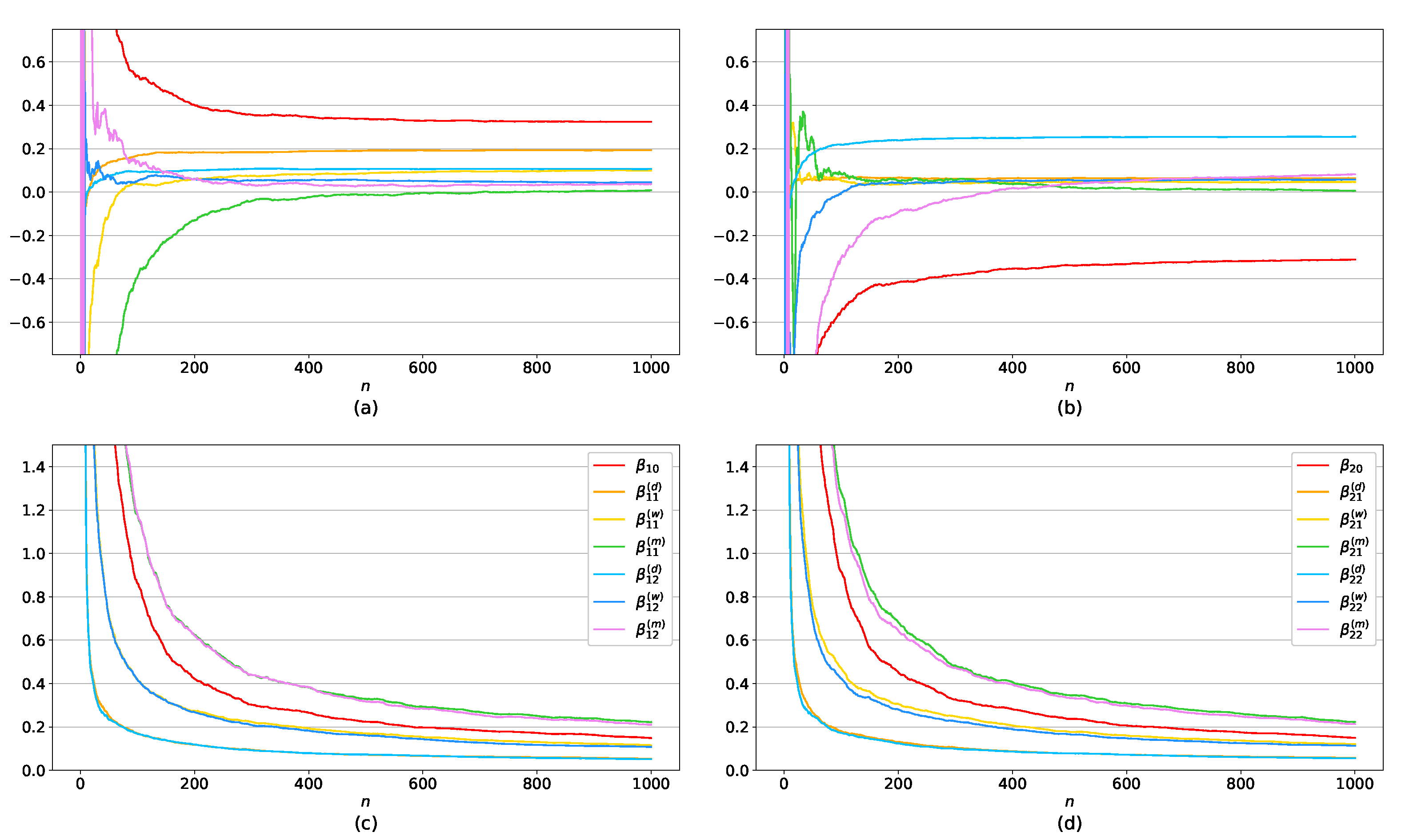
We compute the LSEs for the parameters with replication numbers 500 and give the sample means and standard errors of the 500 estimates in Table 1 and Table 2 with $n=300,600,1000$. It is reported in Tables that sample means are closer to the real values of parameters as well as standard errors decreases as n increases. Additionally, Figure 1 and Figure 2 illustrate plots of sample means (a), (b) and standard errors (c), (d) of the LSEs of the parameters as n increases on the horizontal axis: Figure 1a,c and Figure 2a,c for the estimates of ${\beta }_1$ and Figure 1b,d and Figure 2b,d for the estimates of ${\beta }_2$.

Table 1. Sample mean and standard error of 500 estimates in i.i.d. case.

Parameter			Sample Mean (Standard Error)
			$\mathit{n}=\mathbf{300}$	$\mathit{n}=\mathbf{600}$	$\mathit{n}=\mathbf{1000}$
	${\beta }_{10}$	0.30	0.36 (0.17)	0.33 (0.12)	0.32 (0.08)
	${\beta }_{11}^{\left(d\right)}$	0.20	0.19 (0.07)	0.20 (0.04)	0.20 (0.03)
	${\beta }_{11}^{\left(w\right)}$	0.10	0.08 (0.14)	0.09 (0.10)	0.10 (0.07)
${\beta }_1$	${\beta }_{11}^{\left(m\right)}$	0.05	−0.05 (0.26)	0.00 (0.18)	0.02 (0.13)
	${\beta }_{12}^{\left(d\right)}$	0.10	0.10 (0.07)	0.10 (0.04)	0.10 (0.03)
	${\beta }_{12}^{\left(w\right)}$	0.05	0.06 (0.13)	0.06 (0.09)	0.06 (0.07)
	${\beta }_{12}^{\left(m\right)}$	0.02	0.04 (0.25)	0.02 (0.17)	0.02 (0.12)
	${\beta }_{20}$	−0.30	−0.37 (0.16)	−0.34 (0.12)	−0.32 (0.08)
	${\beta }_{21}^{\left(d\right)}$	0.07	0.06 (0.07)	0.07 (0.05)	0.07 (0.04)
	${\beta }_{21}^{\left(w\right)}$	0.04	0.06 (0.14)	0.05 (0.09)	0.05 (0.07)
${\beta }_2$	${\beta }_{21}^{\left(m\right)}$	0.01	0.01 (0.27)	0.01 (0.18)	0.01 (0.14)
	${\beta }_{22}^{\left(d\right)}$	0.25	0.24 (0.06)	0.25 (0.05)	0.25 (0.04)
	${\beta }_{22}^{\left(w\right)}$	0.07	0.05 (0.14)	0.06 (0.10)	0.06 (0.07)
	${\beta }_{22}^{\left(m\right)}$	0.10	0.00 (0.24)	0.05 (0.16)	0.08 (0.12)

Table 2. Sample mean and standard error of 500 estimates in correlated case.

Parameter			Sample Mean (Standard Error)
			$\mathit{n}=\mathbf{300}$	$\mathit{n}=\mathbf{600}$	$\mathit{n}=\mathbf{1000}$
	${\beta }_{10}$	0.30	0.36 (0.30)	0.33 (0.20)	0.32 (0.15)
	${\beta }_{11}^{\left(d\right)}$	0.20	0.18 (0.09)	0.19 (0.07)	0.19 (0.05)
	${\beta }_{11}^{\left(w\right)}$	0.10	0.07 (0.22)	0.09 (0.15)	0.10 (0.12)
${\beta }_1$	${\beta }_{11}^{\left(m\right)}$	0.05	−0.04 (0.44)	0.00 (0.29)	0.01 (0.22)
	${\beta }_{12}^{\left(d\right)}$	0.10	0.11 (0.09)	0.11 (0.07)	0.11 (0.05)
	${\beta }_{12}^{\left(w\right)}$	0.05	0.05 (0.21)	0.05 (0.14)	0.04 (0.11)
	${\beta }_{12}^{\left(m\right)}$	0.02	0.03 (0.44)	0.03 (0.28)	0.04 (0.21)
	${\beta }_{20}$	−0.30	−0.38 (0.33)	−0.33 (0.21)	−0.31 (0.15)
	${\beta }_{21}^{\left(d\right)}$	0.07	0.06 (0.11)	0.06 (0.07)	0.06 (0.06)
	${\beta }_{21}^{\left(w\right)}$	0.04	0.04 (0.25)	0.05 (0.16)	0.05 (0.12)
${\beta }_2$	${\beta }_{21}^{\left(m\right)}$	0.01	0.06 (0.48)	0.02 (0.31)	0.01 (0.22)
	${\beta }_{22}^{\left(d\right)}$	0.25	0.25 (0.10)	0.25 (0.07)	0.26 (0.06)
	${\beta }_{22}^{\left(w\right)}$	0.07	0.05 (0.23)	0.06 (0.15)	0.06 (0.11)
	${\beta }_{22}^{\left(m\right)}$	0.10	−0.03 (0.47)	0.05 (0.30)	0.08 (0.21)

Figure 1. Sample mean (a,b) and standard error (c,d) of the 500 estimates in i.i.d. case.

Figure 2. Sample mean (a,b) and standard error (c,d) of the 500 estimates in correlated case.

Confidence intervals using the normal approximations in Theorems 2 and 3 with confidence level $95\%$ are constructed: $0.95=P(\widehat{\beta }-z_{0.975}\widehat{se}\le \beta \le \widehat{\beta }+z_{0.975}\widehat{se})$, for each parameter component $\beta$, with its LSE $\widehat{\beta }$ and standard-error estimate $\widehat{se}=\widehat{\sigma }/\sqrt{n}$, where ${\widehat{\sigma }}^2$ is the corresponding (diagonal) component of estimate of asymptotic covariance matrix in Theorems 2 and 3. The confidence intervals of 500 samples as well as the empirical coverage probabilities and average lengths in the i.i.d. 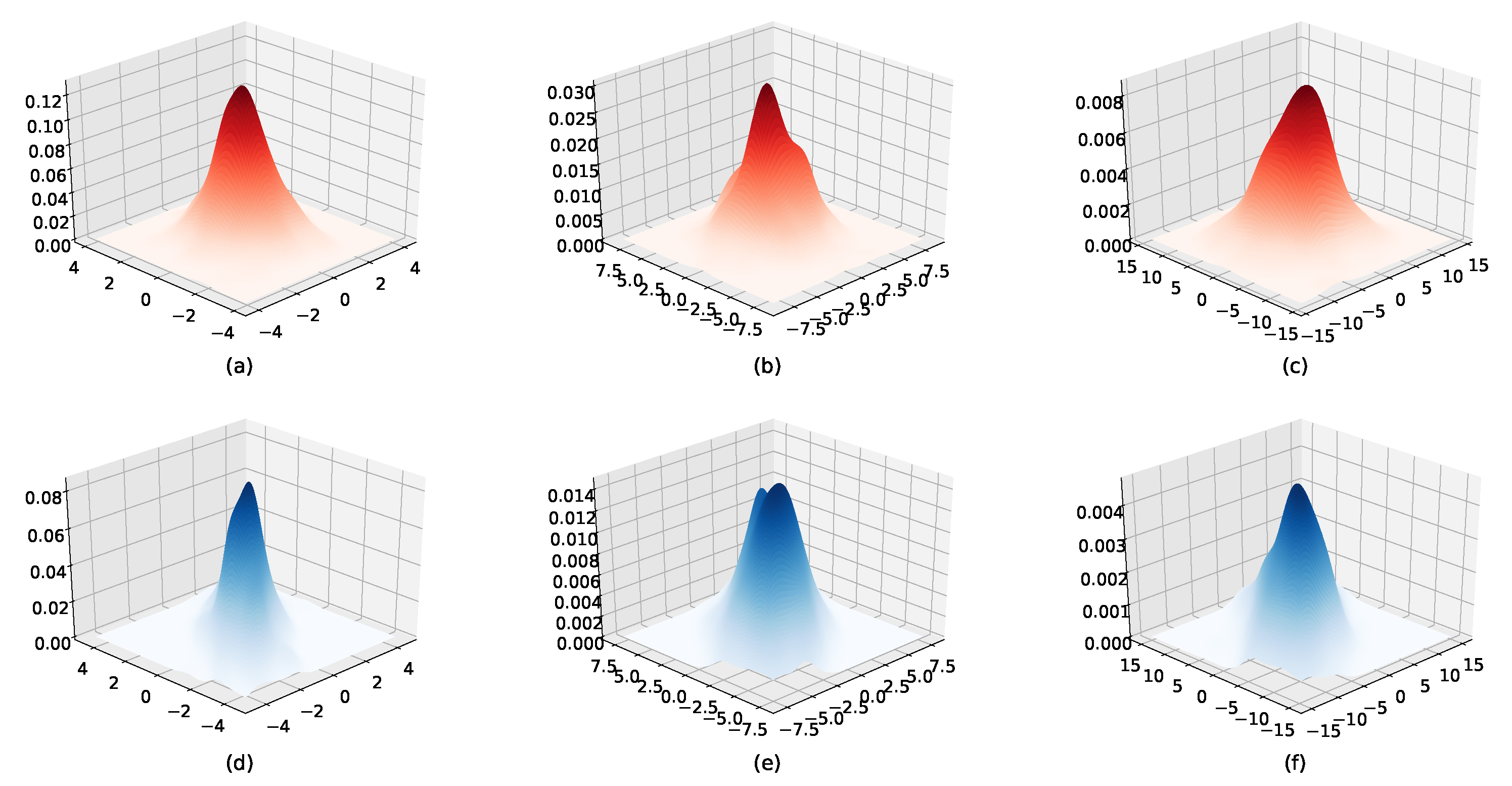error case by the normal approximations are demonstrated in Figure 3, where sample size $n=1000$ and replication number 500 are used. To illustrate the multivariate asymptotic normality, plots of the normal approximations for estimates of some parameters are depicted in Figure 4, and the bivariate normalities of some pairs of two chosen estimates also can be seen in Figure 5. The three figures support normality results established in the theory.

Figure 3. Empirical coverage and average length (in parenthesis) of 95% confidence intervals for seven components of ${\beta }_1$ (left column) and ${\beta }_2$ (right column) in i.i.d. error case. The horizontal dotted line indicates the true value of the parameter in each plot. Confidence intervals that do not contain the parameter are depicted as red color.

Figure 4. Normal approximation of estimates ${\widehat{\beta }}_{11}^{\left(d\right)},{\widehat{\beta }}_{11}^{\left(w\right)},{\widehat{\beta }}_{11}^{\left(m\right)}$ in i.i.d.case (a–c) and correlated case (d–f).

Figure 5. Bivariate normal approximation of some pairs of two chosen estimates (${\widehat{\beta }}_{11}^{\left(d\right)},{\widehat{\beta }}_{21}^{\left(d\right)}),$$({\widehat{\beta }}_{11}^{\left(w\right)},{\widehat{\beta }}_{21}^{\left(w\right)}),$$({\widehat{\beta }}_{11}^{\left(m\right)},{\widehat{\beta }}_{21}^{\left(m\right)})$ in i.i.d.case (a–c) and correlated case (d–f).

As for the exponentially weighted multivariate HAR(3,2) model with ${\beta }_{jk}^{\left(i\right)}=c_{jk}{\lambda }^{i-1}$ in Section 4, the estimates for the common rate are given in Table 3, from which we see that sample means of estimated values are close to the true ones with reasonable standard errors.

Table 3. Sample mean and standard error of 500 estimates in exponentially weighted HAR model.

Parameter		Sample Mean (Standard Error)
		$\mathit{n}=\mathbf{300}$	$\mathit{n}=\mathbf{600}$	$\mathit{n}=\mathbf{1000}$
${\beta }_{10}$	0.10	0.11 (0.09)	0.10 (0.06)	0.10 (0.05)
$c_{11}$	0.30	0.29 (0.05)	0.29 (0.04)	0.30 (0.03)
$c_{12}$	0.20	0.20 (0.05)	0.20 (0.04)	0.20 (0.03)
${\beta }_{20}$	−0.30	−0.33 (0.09)	−0.32 (0.07)	−0.31 (0.05)
$c_{21}$	0.10	0.10 (0.05)	0.10 (0.04)	0.10 (0.03)
$c_{22}$	0.25	0.24 (0.05)	0.25 (0.04)	0.25 (0.03)
$\lambda$	0.50	0.49 (0.23)	0.52 (0.19)	0.50 (0.15)

6. Application

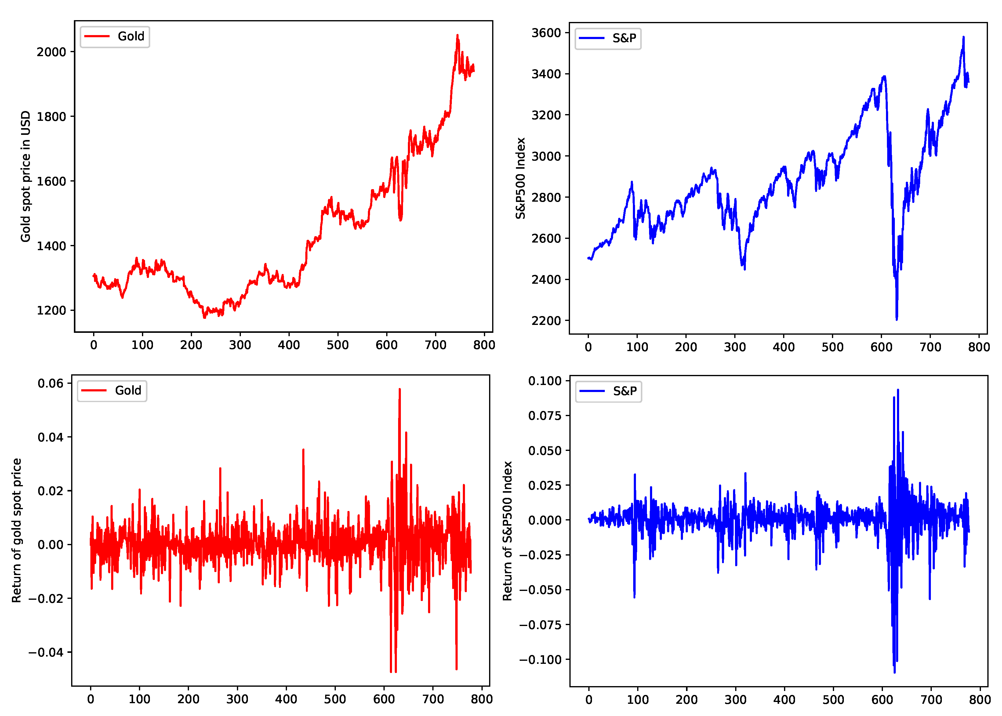
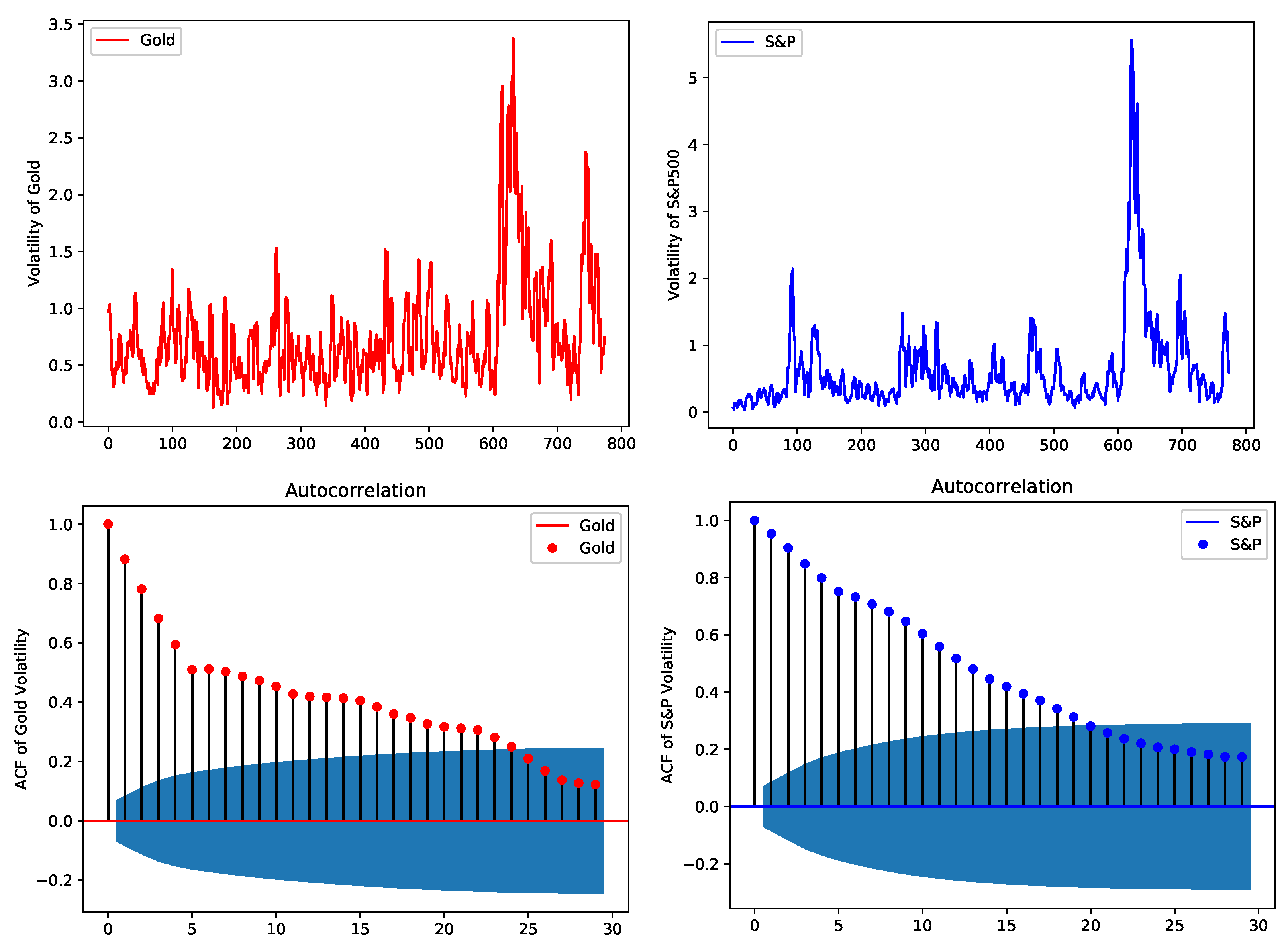
This section addresses empirical data analysis on the Gold spot price and S&P500 index. Their volatility is modeled by bivariate HAR model, using three years of daily closing price, from 18 September 2017 to 17 September 2020, of Gold and S&P500. The three years of Gold price and S&P500 index movement and their log return are shown in Figure 6 while their volatility and autocorrelation coefficients functions (ACFs) in Figure 7.

Figure 6. Gold spot price in USD and its return (in red) and S&P500 index and its return (in blue) against number of days starting from 18 September 2017 to 17 September 2020.

Figure 7. Volatility and ACF for Gold (in red) and S&P 500 (in blue).

We list some critera of MSE, R${}^2$, AIC, BIC in Table 4 for the OLSEs (ordinary least squares estimators) of the bivariate HAR model of order $p=3,4$ by examining the volatility of Gold and S&P500. Conventionally lags of order $p=3,4$ are used for a day ($h_1=1$), a week $(h_2=5)$, a month ($h_3=22$) and a quarter ($h_4=66$) in a HAR model. Nevertheless, in this work, we consider optimal lags in the sense of minimizing MSE of OLSEs for Gold and S&P500 volatility simultaneously. For order $p=3,4$, we choose lags $h_2,\cdots ,h_p$ to satisfy the condition, $1=h_1<h_2<\cdots <h_p<\overline{h}$ for some large $\overline{h}$, so that the sum of the two mean squared residuals of the OLSEs for the volatility of Gold and S&P500 is minimized. As a result, we found optimal lags $(h_1,h_2,h_3)=(1,5,6)$ for $p=3$ with (MSE${}_{\mathrm{Gold}}$, MSE${}_{\mathrm{S\&P}})=(0.0461,0.0387)$ and $(h_1,h_2,h_3,h_4)=(1,3,6,7)$ for $p=4$ with (MSE${}_{\mathrm{Gold}}$, MSE${}_{\mathrm{S\&P}})=(0.0488,0.0410)$. In Table 4, we compare our optimal lags with the conventional lags in different criteria. In all cases considered, our selection of optimal lags $(h_1,h_2,h_3)=(1,5,6)$ with $p=3$ turns out to be the best.

Table 4. OLSEs in the bivariate HAR($p,2)$ model on volatility of Gold and S&P500.

		Gold				S&P500
		MSE	R${}^2$	AIC	BIC	MSE	R${}^2$	AIC	BIC
$p=3$	$(1,5,22)$	0.0492	0.790	−117.0	−84.68	0.0420	0.910	−236.6	−204.2
	$(1,5,6)$	0.0461 *	0.801 *	−169.8 *	−137.3 *	0.0387 *	0.916 *	−303.2 *	−270.7 *
$p=4$	$(1,5,22,66)$	0.0519	0.789	−73.30	−32.24	0.0448	0.909	−180.3	−139.3
	$(1,3,6,7)$	0.0488	0.791	−128.1	−86.28	0.0410	0.912	−264.4	−222.6

* Denotes the best.

Therefore we report estimation results of the HAR(3,2) model with $(h_1,h_2,h_3)=(1,5,6)$ for the volatilities of Gold and S&P500 in Table 5, where coefficients estimates, standard errors and 95% confidence intervals are provided. In Figure 8, two plots of the bivariate HAR(3,2) fitted model by the OLSEs for this optimal case on the datasets of Gold and S&P volatilities are depicted along with residuals. We see that the bivariate HAR(3,2) fittings are similar to the real volatility plots of both datasets as reported upon the criterions.

Table 5. Estimation results for Gold and S&P500 using HAR(3,2) with $(h_1,h_2,h_3)=(1,5,6)$.

Parameter		Gold ($\mathit{j}=1$)		S&P ($\mathit{j}=2$)
		Coeff. est.(s.e.)	(95% C.I.)	Coeff. est.(s.e.)	(95% C.I.)
	${\beta }_{j0}$	0.0790 (0.016)	(0.047, 0.111)	−0.0088 (0.015)	(−0.038, 0.021)
	${\beta }_{j1}^{\left(1\right)}$	0.9751 (0.038)	(0.901, 1.049)	0.0534 (0.034)	(−0.014, 0.121)
	${\beta }_{j1}^{\left(2\right)}$	−1.0822 (0.187)	(−1.450, −0.714)	−0.4278 (0.172)	(−0.765, −0.091)
${\beta }_j$	${\beta }_{j1}^{\left(3\right)}$	0.9301 (0.175)	(0.586, 1.274)	0.4458 (0.161)	(0.130, 0.761)
	${\beta }_{j2}^{\left(1\right)}$	0.1478 (0.039)	(0.071, 0.225)	1.1153 (0.036)	(1.045, 1.186)
	${\beta }_{j2}^{\left(2\right)}$	−0.6484 (0.198)	(−1.036, −0.261)	−1.1196 (0.181)	(−1.475, −0.764)
	${\beta }_{j2}^{\left(3\right)}$	0.5879 (0.179)	(0.237, 0.939)	0.9338 (0.164)	(0.612, 1.256)

Figure 8. Fitted HAR model and residual using OLSE for the volatility of Gold and S&P500.

7. Conclusions

Due to the cross-correlation of multiple assets and spillover effect of volatility in the financial market, a multivariate heterogeneous autoregressive-realized volatility (HAR-RV) model has attained much attention recently. In the multivariate HAR model, its stationarity is discussed and estimation problems are studied. We first investigate the strictly stationarity solution of the multivariate HAR model and second develop the asymptotic normality theory for the least squares estimates (LSEs) with i.i.d. and correlated errors, respectively. Third, we propose an exponentially weighted multivariate HAR model and estimate its common exponential decay rate. In a Monte-Carlo experiment, performances of the LSEs are numerically illustrated with sample mean and standard error of the estimates as well as empirical coverage and average length of confidence intervals by using the normal approximation. In addition, as a real data example, volatilities of Gold spot price and S&P500 index during recent three years are used to analyze in a bivariate HAR model. The coefficient estimates and confidence intervals are found in the bivariate HAR model of volatility of Gold and S&P500, along with choosing optimal lags, and it is shown that the bivariate HAR model with the proposed optimal lags is well matched with the volatility of the financial data.

We suggest some problems on the multivariate HAR model. As we proposed before, the exponentially weighted HAR models with decay rates are of interest owing to reduced numbers of parameters as well as the long-memory property. In modeling the multivariate HAR model, testing whether the HAR coefficients have exponentially weighted decay rates or not and furthermore whether multiple assets have a common decay rate or not might provide statistically useful tools to analyze the time series model. In follow-up studies we will deal with the hypotheses tests by constructing the test statistics and establishing the null limiting distribution. Finally, we mention that in a multivariate HAR model with heteroscedasticity errors, asymptotic properties of the estimates differ from the existing results, and thus we will derive the asymptotic theory on the HAR models in the presence of dynamic heteroscedasticity. In this case, financial market data can be represented more remarkably and hence forecasting volatility with forecast accuracy will be carried out in the further research.