Article

Distributed Fusion Estimation with Sensor Gain Degradation and Markovian Delays

by
María Jesús García-Ligero
,
Aurora Hermoso-Carazo
*,† and
Josefa Linares-Pérez
Departamento de Estadística e I. O., Universidad de Granada, Avda Fuentenueva s/n, 18071 Granada, Spain
*
Author to whom correspondence should be addressed.
These authors contributed equally to this work.
Mathematics 2020, 8(11), 1948; https://doi.org/10.3390/math8111948
Submission received: 25 September 2020 / Revised: 30 October 2020 / Accepted: 31 October 2020 / Published: 4 November 2020
(This article belongs to the Special Issue Stochastic Statistics and Modeling)

Abstract

:
This paper investigates the distributed fusion estimation of a signal for a class of multi-sensor systems with random uncertainties both in the sensor outputs and during the transmission connections. The measured outputs are assumed to be affected by multiplicative noises, which degrade the signal, and delays may occur during transmission. These uncertainties are commonly described by means of independent Bernoulli random variables. In the present paper, the model is generalised in two directions: ( i ) at each sensor, the degradation in the measurements is modelled by sequences of random variables with arbitrary distribution over the interval [0, 1]; ( i i ) transmission delays are described using three-state homogeneous Markov chains (Markovian delays), thus modelling dependence at different sampling times. Assuming that the measurement noises are correlated and cross-correlated at both simultaneous and consecutive sampling times, and that the evolution of the signal process is unknown, we address the problem of signal estimation in terms of covariances, using the following distributed fusion method. First, the local filtering and fixed-point smoothing algorithms are obtained by an innovation approach. Then, the corresponding distributed fusion estimators are obtained as a matrix-weighted linear combination of the local ones, using the mean squared error as the criterion of optimality. Finally, the efficiency of the algorithms obtained, measured by estimation error covariance matrices, is shown by a numerical simulation example.

1. Introduction

Sensor network systems are of great research interest because of their potential application in a wide range of fields, including target tracking, integrated navigation, military surveillance, mobile robotics and traffic control. In a multi-sensor environment, the information provided by each sensor is transmitted to a processing centre where it is combined or fused by different methods according to how the question of fusion estimation is addressed. The information provided by multiple sensors is normally processed by one of the following methods: either it is centralised, with the sensor outputs being sent to a central processor to be fused, or it is distributed, by a process in which the local estimators are derived and then sent to the processing centre. Centralised fusion estimation provides optimal estimators when all the sensors are faultless, but has the disadvantage that its application imposes high computational costs and a heavy communication burden, especially when a large number of sensors must be considered. Distributed fusion estimation, on the other hand, does not generally provide optimal estimators, but reduces the computational load and is usually more suitable for large-scale sensor networks with random transmission failures, because of its parallel structure. Due to these advantages, the use of distributed fusion estimation in multiple-sensor systems has attracted considerable interest in recent years, with various approaches being taken; for detailed information, see [1,2,3,4,5,6,7] and the references therein.
In a multi-sensor environment, failures may occur both in signal measurements and during the transmission of measured outputs. In the first of these respects, problems such as aging, temporary failure or high levels of background noise may provoke, for example, missing measurements or stochastic sensor gain degradation. The missing measurement phenomenon has received considerable attention, and many studies have been conducted to determine specific distributed estimation algorithms, using different approaches (see [8,9,10]). Usually, a common way to model missing measurements is to consider variables with Bernoulli distribution whose values zero and one represent that the signal is completely absent or completely present in the measurement. However, such an assumption is restrictive in some practical situations since the communications in networked systems are not always perfect and there may be measurement fades/degrades; in such cases, the received measurement may contain only partial information about the signal. The signal estimation problem in case of sensor gain degradation in a multi-sensor environment has not been so extensively investigated, even though the phenomenon of sensor gain degradation (sensor fading measurement) occurs frequently in engineering practice, for example, in thermal sensors for vehicles or in platform-mounted sonar arrays receiving acoustic signals from the ocean. As in the case of missing measurements, conventional estimation algorithms are not applicable to the phenomenon of sensor gain degradation, and studies have been undertaken to obtain estimation algorithms in this situation. For example, Liu et al. [11] studied the optimal filtering problem for networked time-varying systems with stochastic gain degradation, using a recursive matrix equation approach, Liu et al. [12] obtained a minimum variance filtering algorithm for a class of time-varying systems and Liu et al. [13] designed filters distributed over a wireless sensor network located within a given sporadic communication topology.
Furthermore, the measured outputs may be transmitted to the processing centre via communication networks through imperfect channels or be affected by network congestion, and either of these problems can produce random uncertainties in the processed measurements, such as random delays. The possible influence of random delays on the performance of the estimators makes it necessary to develop new estimation algorithms that take account of this problem. For random delays modelled by independent Bernoulli random variables, which is a common assumption, various distributed fusion estimation algorithms have been derived (see, for example, [14,15,16,17,18]). Nevertheless, in real-world communication systems, current delays are usually correlated with previous ones. In this context, assuming that the random delays are modelled by Bernoulli random variables correlated at consecutive sampling times, distributed estimation algorithms were developed by [19,20]. A more general approach, in which the correlation is considered at different times, is to model the delays by means of Markov chains. Under this hypothesis, the estimation problem has been addressed considering a single sensor (see [21,22,23,24]), but to the best of our knowledge, it has not been extensively investigated in a multi-sensor environment. Relevant papers in this context include Ge et al. [25], who investigated the distributed estimation problem for continuous-time linear systems over sensor networks with heterogeneous Markovian coupling intercommunication delays, and García-Ligero et al. [26], who proposed fusion filtering and smoothing algorithms to estimate a signal from one-step delayed measurements with random delays modelled by Markov chains. Also, when the network connectivity is given by topology, relevant works on the consensus problem of linear continuous-time multi-agent systems, as [27,28], have considered continuous-time homogeneous Markov processes with finite state space to describe the communication topology among agents, corresponding each communication graph to a state of the Markov process.
In some conventional algorithms in network systems, the additive noises are assumed white and uncorrelated between the different sensors. However, in many practical applications of multisensor systems, a more realistic scenario is to consider that the noises at different sensors are cross-correlated. For example, in wireless communication, speech enhancement systems or global navigation satellite systems, the noises are usually correlated and cross-correlated. For this reason, research into sensor network systems under the assumption of correlated and/or cross-correlated noises is a promising field of activity, and numerous papers incorporating this assumption are now appearing (see, for example, [29,30,31,32,33]).
In this paper, our aim is to investigate the distributed fusion estimation problem in networked systems subject to stochastic sensor gain degradation and to random transmission delays of one or two steps. At each sensor, the deterioration of the measured output is modelled by sequences of arbitrary variables, with values in the range [0, 1], corresponding to a possible partial or total loss of the signal. In addition, the measurement noises are assumed to be correlated and cross-correlated at the same and at consecutive sampling times. The delays that can occur during the transmission of the measurements from each sensor to the local processing centre are described by different homogeneous Markov chains. In this context, we can derive least-squares distributed linear filter and fixed-point smoothers, without requiring full knowledge of the signal evolution model, only the first and second-order moments of the processes involved in the multi-sensor system are needed. In this process, we first use an innovation approach to derive algorithms for local estimators, including filter and fixed-point smoothers. This method simplifies the derivation because the innovation is a white process. The distributed fusion filter and the fixed-point smoothers are then obtained as the matrix-weighted linear combinations of the corresponding local estimators using the mean squared error as the optimality criterion.
The rest of this paper is structured as follows. In Section 2, we present the model considered and detail the assumptions according to which the distributed fusion estimation problem is addressed. In Section 3, distributed filtering and fixed-point smoothing estimators, together with their estimation error covariance matrices, are derived. Using an innovation approach, local least-squares linear filtering and smoothing algorithms are obtained for each sensor, and the cross-correlation matrices between any two local estimators are then calculated in order to derive the distributed fusion estimators. Section 4 provides a simulation example to illustrate the applicability of the proposed algorithms and analyses the performance of the estimators. Finally, we summarise the main conclusions drawn.
Notation. 
The usual notation is used in this paper. Thus, R n × m denotes the set of all n × m matrices. ( C 1 | | C n ) denotes a matrix partitioned into submatrices C 1 , , C n , d i a g ( A i ) i I stands for a block-diagonal matrix whose blocks are the sub-matrices A i , with i varying in the set of indices I, and I n is n × n identity matrix. If the dimensions of vectors or matrices are not explicitly stated, they are assumed to be compatible with algebraic operations. The Kronecker product is denoted by the symbol ⊗, the minimum and maximum values of two real numbers are represented, respectively, by c d and c d , c , d R , and the Kronecker delta function is denoted as δ k , s . For simplicity, F k = F k , k is used for any function F k , s depending on the time instants k and s; analogously, if L ( i j ) is a function depending on sensors i and j , we is written as L ( i ) = L ( i i ) .

2. Problem Statement and Model Description

In this study, our aim is to investigate the least-squares (LS) linear estimation of a discrete-time random signal in a multi-sensor environment, using the distributed fusion method. At each sensor, problems such as aging, temporary failure or excessive background noise may deteriorate the signal measurement, causing a partial loss of information at the measured outputs. In addition, the measurement noises are assumed to be correlated and one-step cross-correlated both in a single sensor and between different sensors.
In order to perform the signal estimation, each sensor transmits its outputs to a local processor via communication channels; during this transmission, faults may occur due to limited communication bandwidth, congestion or defects in the channels, which can produce random delays in the processed measurements.
In this context, the LS distributed linear filter and fixed-point smoother of the signal are derived by a covariance-based approach; that is, we assume that the signal evolution model is unknown and that only the first and second order moments are known. Specifically:
Assumption 1.
The n x -dimensional signal process, x k , k 1 , has a zero mean and its autocovariance function is expressed in a separable form as follows,
E x k x h T = A k B h T , h k ,
where A k , B h R n x × M are known matrices.
Consider m sensors and assume that, at each one, the sensor gain is randomly degraded and, therefore, partially deteriorated measured outputs may be obtained. Under this assumption, the measured outputs, z k ( i ) R n z , are described by
z k ( i ) = γ k ( i ) H k ( i ) x k + v k ( i ) , k 1 , i = 1 , , m ,
where, for i = 1 , , m , the random variables γ k ( i ) quantify the sensor gain degradation, H k ( i ) are known matrices and v k ( i ) are measurement noises. The following assumptions are made concerning the measurement model (1):
Assumption 2.
The multiplicative noises γ k ( i ) , k 1 , i = 1 , , m , are independent sequences of independent random variables taking values in [ 0 , 1 ] , with known means and variances, E γ k ( i ) = γ ¯ k ( i ) and Var γ k ( i ) = σ k 2 ( i ) , k 1 .
Note that modelling the sensor gain degradation by arbitrary random variables taking values in the interval [ 0 , 1 ] describes not only partially degraded signals but also conventional missing signals (by considering only the values 0 and 1 for γ k ( i ) ), see, for example, Caballero-Águila et al. [20]. Therefore, the current model generalises the missing measurement model.
Assumption 3.
The measurement noises v k ( i ) , k 1 , i = 1 , , m , have zero-mean and second-order moments given by E v k ( i ) v h ( j ) T = R k ( i j ) δ k , h + R k , k 1 ( i j ) δ k 1 , h , h k .
Note that this assumption is weaker and more realistic than the usual hypothesis of independent white measurement noises and reflects to conditions which occur in many real-life situations; for example, in wireless communication, speech enhancement systems or global navigation satellite systems, the measurement noises are usually correlated and cross-correlated.
As commented above, during the transmission of measurements from each sensor to its processing centre, random delays frequently occur. In this paper, the absence or presence of transmissions delays, and their magnitudes, at each sensor are modelled by random variables θ k ( i ) , k 1 , that take values in E = 0 , 1 , 2 , describing whether the measures arrive on time or are delayed by one or two sampling times. Specifically, if θ k ( i ) = a , a = 1 , 2 , this means that the k-th measurement of the i-th sensor is delayed by a sampling periods; otherwise, if θ k ( i ) = 0 , there is no delay in the arrival.
Then, the measurements received, which are denoted by y k ( i ) , k 1 , are described as in García-Ligero et al. [24]:
y k ( i ) = a = 0 ( k 1 ) 2 δ θ k ( i ) , a z k a ( i ) , k 1 , i = 1 , , m .
Assumption 4.
θ k ( i ) , k 1 , i = 1 , , m , are independent homogeneous Markov chains with the same state space, E = 0 , 1 , 2 , known initial distributions π 1 , a ( i ) = P ( θ 1 ( i ) = a ) , a E , and transition probability matrices P 1 ( i ) = p 1 , [ a , b ] ( i ) a , b E , where p 1 , [ a , b ] ( i ) = P ( θ h + 1 ( i ) = b / θ h ( i ) = a ) , h 1 , a , b E .
Finally, the following hypothesis about the signal and processes involved in the measurement model is assumed in the derivation of the LS linear estimators.
Assumption 5.
For each i = 1 , , m , x k , k 1 , γ k ( i ) , k 1 , v k ( i ) , k 1 and θ k ( i ) , k 1 , are mutually independent.

3. Distribution Fusion Estimation Problem

In this section, we address the LS linear estimation of a signal in a multi-sensor environment, using the distributed fusion method. This method involves first determining, in each local processor, LS linear estimators based on the delayed measurements received from the sensor itself. Then, all the local estimators are transmitted, over perfect connections, to a fusion centre from which the distributed estimator is obtained.

3.1. Local Filter and Fixed-Smoothing Algorithms

The fusion method is applied as follows; for each i = 1 , , m , we determine the local filters and fixed-point smoothers for the model described by (1) and (2) using an innovation approach. As it is known, the whiteness of the innovation process simplifies the derivation of the estimation algorithms, as well as the algorithms themselves, thus providing computational advantages. The innovation treatment is based on the equivalence existing between the observation process { y k ( i ) ; k 1 } and the innovations { μ k ( i ) ; k 1 } , which are defined as μ k ( i ) = y k ( i ) y ^ k / k 1 ( i ) , where y ^ k / k 1 ( i ) is the LS linear estimator of y k ( i ) from the previous observations, y 1 ( i ) , , y k 1 ( i ) . Since both processes provide the same information, the LS linear estimator of a random vector u k ( i ) based on the observations y 1 ( i ) , , y L ( i ) , denoted by u ^ k / L ( i ) , is expressed as a linear combination of the innovations μ 1 ( i ) , , μ L ( i ) ; specifically:
u ^ k / L ( i ) = h = 1 L E u k ( i ) μ h ( i ) T Σ μ h ( i ) 1 μ h ( i ) , k , L 1 ,
where Σ μ h ( i ) = E μ h ( i ) μ h ( i ) T denotes the innovation covariance matrices.
The observation model in each individual sensor is, for vectorial observations, the same as was considered in García-Ligero et al. [24]. Therefore, the derivation of the local estimation algorithms is analogous to that performed in the paper cited and the proofs of the local LS linear filtering and fixed-smoothing algorithms can be omitted.
In order to simplify the expressions of the algorithms, the following notations are used:
A k ( i ) = γ ¯ k ( i ) H k ( i ) A k | γ ¯ k 1 ( i ) H k 1 ( i ) A k 1 | γ ¯ k 2 ( i ) H k 2 ( i ) A k 2 P k ( i ) I M T , k 1 , B k ( i ) = γ ¯ k ( i ) H k ( i ) B k | γ ¯ k 1 ( i ) H k 1 ( i ) B k 1 | γ ¯ k 2 ( i ) H k 2 ( i ) B k 2 P k ( i ) P k ( i ) 1 I M , k 1 , where γ ¯ k ( i ) H k ( i ) C k = 0 f o r k = 1 , 0 , a n d C k = A k , B k , P k ( i ) = p k , [ a , b ] ( i ) a , b E with p k , [ a , b ] ( i ) = P θ h + k ( i ) = b / θ h ( i ) = a , k , h 1 ; a , b E , P k ( i ) = d i a g π k , a ( i ) I M a E , where π k , a ( i ) = P ( θ k ( i ) = a ) , a E , k 1 , H D k ( i ) = a = 0 ( k 1 ) 2 π k , a ( i ) γ ¯ k a ( i ) H k a ( i ) D k a , k 1 , D = A , B .

3.1.1. Local LS Linear Filtering Algorithm

Under the model assumptions, for i = 1 , , m , the local filters, x ^ k / k ( i ) , and their error covariance matrices, Σ k / k ( i ) = E [ ( x k x ^ k / k ( i ) ) ( x k x ^ k / k ( i ) ) T ] , are obtained as
x ^ k / k ( i ) = A k O k x ( i ) , k 1 ,
Σ k / k ( i ) = A k ( B k T r k x ( i ) A k T ) , k 1 .
The vectors O k d ( i ) , d = x , y , are recursively calculated as
O k d ( i ) = O k 1 d ( i ) + J k d ( i ) Π k ( i ) 1 μ k ( i ) , k 1 ; O 0 d ( i ) = 0 ,
where the matrices J k d ( i ) = E O k d ( i ) μ k ( i ) T , d = x , y , satisfy
J k x ( i ) = H B k ( i ) T r k 1 x y ( i ) A k ( i ) T ( 1 δ k , 1 ) s = ( k 3 ) 1 k 1 J s x ( i ) Π s ( i ) 1 G k , s ( i ) T , k 1 ,
and
J k y ( i ) = B k ( i ) T r k 1 y ( i ) A k ( i ) T ( 1 δ k , 1 ) s = ( k 3 ) 1 k 1 J s y ( i ) Π s ( i ) 1 G k , s ( i ) T , k 1 .
The matrices r k d e ( i ) = E [ O k d ( i ) O k e ( i ) T ] , d , e = x , y , are obtained by
r k d e ( i ) = r k 1 d e ( i ) + J k d ( i ) Π k ( i ) 1 J k e ( i ) T , k 1 ; r 0 d e ( i ) = 0 .
The innovations μ k ( i ) = y k ( i ) y ^ k / k 1 ( i ) and their covariance matrices Π k ( i ) = E [ μ k ( i ) μ k ( i ) T ] are given by
μ k ( i ) = y k ( i ) A k ( i ) O k 1 y ( i ) ( 1 δ k , 1 ) s = ( k 3 ) 1 k 1 G k , s ( i ) Π s ( i ) 1 μ s ( i ) , k 1 ,
Π k ( i ) = a = 0 ( k 1 ) 2 π k , a ( i ) ( σ k a 2 ( i ) H k a ( i ) A k a B k a T H k a ( i ) T + R k a ( i ) ) + A k ( i ) J k y ( i ) ( 1 δ k , 1 ) s = ( k 3 ) 1 k 1 G k , s ( i ) Π s ( i ) 1 ( A k ( i ) J s y ( i ) + G k , s ( i ) ) T , k 1 ,
where
G k , k 1 ( i ) = F k , k 1 ( i ) ( 1 δ k , 2 ) s = ( k 3 ) 1 k 2 G k , s ( i ) Π s ( i ) 1 ( A k 1 ( i ) J s y ( i ) + G k 1 , s ( i ) ) T , k 2 , G k , k 2 ( i ) = F k , k 2 ( i ) ( 1 δ k , 3 ) G k , k 3 ( i ) Π k 3 ( i ) 1 ( A k 2 ( i ) J k 3 y ( i ) + G k 2 , k 3 ( i ) ) T , k 3 , G k , k 3 ( i ) = F k , k 3 ( i ) , k 4 ,
and
F k , k 1 ( i ) = ( 1 δ k , 2 ) π k 1 , 0 ( i ) p 1 , [ 0 , 2 ] ( i ) γ ¯ k 2 ( i ) γ ¯ k 1 ( i ) H k 2 ( i ) ( B k 2 A k 1 T A k 2 B k 1 T ) H k 1 ( i ) T + a = 1 ( k 1 ) 2 π k 1 , a 1 ( i ) p 1 , [ ( a 1 ) , a ] ( i ) σ k a 2 ( i ) H k a ( i ) A k a B k a T H k a ( i ) T + a = 0 ( k 1 ) 2 b = 0 ( k 2 ) a π k 1 , b ( i ) p 1 , [ b , a ] ( i ) R k a , k 1 b ( i ) , k 2 , F k , k 2 ( i ) = π k 2 , 0 ( i ) p 2 , [ 0 , 2 ] ( i ) σ k 2 2 ( i ) H k 2 ( i ) A k 2 B k 2 T H k 2 ( i ) T + a = 1 2 b = 0 ( k 3 ) ( a 1 ) π k 2 , b ( i ) p 2 , [ b , a ] ( i ) R k a , k 2 b ( i ) , k 3 , F k , k 3 ( i ) = π k 3 , 0 ( i ) p 3 , [ 0 , 2 ] ( i ) R k 2 , k 3 ( i ) , k 4 .
 □
Next, for i = 1 , , m , a recursive fixed-point smoothing algorithm of the signal x k based on y 1 ( i ) , , y S ( i ) , S = k + 1 , k + 2 , , is provided.

3.1.2. Local LS Linear Fixed-Smoothing Algorithm

Under the model assumptions, for i = 1 , , m , the local fixed-point smoothers, x ^ k / S ( i ) , and their error covariance matrices, Σ k / S ( i ) are calculated as follows:
x ^ k / S ( i ) = x ^ k / S 1 ( i ) + X k , S ( i ) Π S ( i ) 1 μ S ( i ) , S > k 1 ,
Σ k / S ( i ) = Σ k / S 1 ( i ) X k , S ( i ) Π S ( i ) 1 X k , S ( i ) T , S > k 1 ,
with initial conditions x ^ k / k ( i ) and Σ k / k ( i ) given by (3) and (4), respectively.
The coefficients X k , S ( i ) = E x k μ S ( i ) T are obtained as
X k , S ( i ) = B k H A S ( i ) T E k , S 1 y ( i ) A S ( i ) T h = ( S 3 ) 1 S 1 X k , h ( i ) Π h ( i ) 1 G S , h ( i ) T + ( 1 δ k , 1 ) δ k + 1 , S π k + 1 , 2 ( i ) γ ¯ k 1 ( i ) ( A k B k 1 T B k A k 1 T ) H k 1 ( i ) T , S > k 1 ; X k , h ( i ) = A k J h x ( i ) , h = k 2 , k 1 , k ,
where the matrices E k , S y ( i ) = E x ^ k / S ( i ) O S y ( i ) T satisfy the following recursive expression
E k , S y ( i ) = E k , S 1 y ( i ) + X k , S ( i ) Π S ( i ) 1 J S y ( i ) T , S > k 1 ; E k y ( i ) = A k r k x y ( i ) , k 1 .

3.2. Distributed Ls Linear Algorithms

In this subsection, distributed filter and fixed-point smoothers, x ^ k / S D , S k , are derived as the matrix-weighted linear combinations of the corresponding local estimators, x ^ k / S ( i ) , i = 1 , , m , minimising the mean squared error; that is, x ^ k / S D = F k / S X ^ k / S = i = 1 m F k / S ( i ) x ^ k / S ( i ) , where X ^ k / S = ( x ^ k / S ( 1 ) T , , x ^ k / S ( m ) T ) T and F k / S = ( F k / S ( 1 ) , , F k / S ( m ) ) minimises E ( x k F k / S X ^ k / S ) T ( x k F k / S X ^ k / S ) .
The solution to this problem, as shown by García-Ligero et al. [26], is given by
F k / S o p t = E x k X ^ k / S T E [ X ^ k / S X ^ k / S T ] 1 , S k ; k 1 ,
and, then, the optimal distributed estimator of x k is
x ^ k / S D = E x k X ^ k / S T E [ X ^ k / S X ^ k / S T ] 1 X ^ k / S , S k ; k 1 .
Theorem 1.
Let x ^ k / S ( i ) , i = 1 , , m , be the local estimators given by (3) and (7); then the optimal distributed fusion estimators x ^ k / S D , filters and fixed-point smoothers, are given by
x ^ k / S D = K k / S ( 1 ) , , K k / S ( m ) K k / S ( i j ) 1 X ^ k / S , S k ; k 1 ,
where K k / S ( i j ) = E x ^ k / S ( i ) x ^ k / S ( j ) T , i , j = 1 , , m .
The estimation error covariance matrices, Σ k / S D = E ( x k x ^ k / S D ) ( x k x ^ k / S D ) T , are given by
Σ k / S D = A k B S T K k / S ( 1 ) , , K k / S ( m ) K k / S ( i j ) 1 K k / S ( 1 ) , , K k / S ( m ) T , S k ; k 1 .
Proof. 
By the Orthogonal Projection Lemma (OPL), E x k x ^ k / S ( i ) T = K k / S ( i ) and, consequently, E x k X ^ k / S T = ( K k / S ( 1 ) , , K k / S ( m ) ) . Then, since E X ^ k / S X ^ k / S T = K k / S ( i j ) i , j = 1 , , m , expression (9) for the distributed estimator is derived from (8). The estimation error covariance matrix (10) is immediately obtained from Assumption 1 and (9). □
Note that expressions (9) and (10) require the knowledge of the cross-correlation matrices between any two local estimators, K k / S ( i j ) , i , j = 1 , , m . Algorithms to obtain these matrices are provided in Theorems 2 and 3 for the filters and smoothers, respectively.
Theorem 2.
For any i , j = 1 , m , the cross-correlation matrices between any two local filters, K k / k ( i j ) = E x ^ k / k ( i ) x ^ k / k ( j ) T , k 1 , are obtained by
K k / k ( i j ) = A k r k x ( i j ) A k T , k 1 .
The covariance matrices r k d e ( i j ) = E O k d ( i ) O k e ( j ) T , d , e = x , y , verify the following recursive relation:
r k d e ( i j ) = r k 1 d e ( i j ) + ( 1 δ k , 1 ) J k 1 , k d ( i j ) Π k ( j ) 1 J k e ( j ) T + J k d ( i ) Π k ( i ) 1 J k e ( j i ) T , k 1 ; r 0 d e ( i j ) = 0 ,
where J k 1 , k d ( i j ) = E O k 1 d ( i ) μ k ( j ) T , d = x , y , are given by
J k 1 , k d ( i j ) = D k , k 1 d ( j i ) T r k 1 d y ( i j ) A k ( j ) T h = ( k 3 ) 1 k 1 J k 1 , h d ( i j ) Π h ( j ) 1 G k , h ( j ) T , k 2 .
The matrices J k , k d ( i j ) = E O k d ( i ) μ k ( j ) T , d = x , y , in the sum of (13) are calculated by
J k , k d ( i j ) = ( 1 δ k , 1 ) J k 1 , k d ( i j ) + J k d ( i ) Π k ( i ) 1 Π k , k ( i j ) , k = k 2 , k 1 , k ; k 1 .
The matrices D k , k 1 d ( i j ) = E y k ( i ) O k 1 d ( j ) T , d = x , y , in expression (13) are obtained as follows
D k , k 1 d ( i j ) = H A k ( i ) r k 2 x d ( j ) + ( 1 δ k , 2 ) a = 1 2 π k , a ( i ) V k a , k 2 d ( i j ) + Y k , k 1 ( i j ) Π k 1 ( j ) 1 J k 1 d ( j ) T , k 2 .
The matrices V k , k d ( i j ) = E v k ( i ) O k d ( j ) T , d = x , y , in the sum of (15) are given by
V k , k d ( i j ) = h = ( k 1 ) 1 k V k , h ( i j ) Π h ( j ) 1 J h d ( j ) T , k = k 1 , k ; k 1 ,
where V k , k ( i j ) = E v k ( i ) μ k ( j ) T , k = k 1 , k , k + 1 , k + 2 ; k 1 , are calculated as
V k , k ( i j ) = a = ( k k 1 ) 0 ( k k + 1 ) ( k 1 ) 2 π k , a ( j ) R k , k a ( i j ) ( 1 δ k 1 , k ) h = ( k 1 ) 1 k 1 V k , h ( i j ) Π h ( j ) 1 Y k , h ( j ) T .
The innovation cross-covariance matrices Π k , k ( i j ) = E μ k ( i ) μ k ( j ) T in expression (14) satisfy
Π k , k ( i j ) = Y k , k ( i j ) ( 1 δ k , 1 ) A k ( i ) J k 1 , k y ( i j ) + h = ( k 3 ) 1 k 1 G k , h ( i ) Π h ( i ) 1 Π h , k ( i j ) , k = k 3 , k 2 , k 1 , k ; k 1 ,
where the coefficients Y k , k ( i j ) = E y k ( i ) μ k ( j ) T are given by
Y k , k ( i j ) = a = 0 ( k 1 ) 2 π k , a ( i ) γ ¯ k a ( i ) H k a ( i ) X k a , k ( j ) + V k a , k ( i j ) , k = k 3 , k 2 , k 1 , k ; k 1 .
Proof. 
See Appendix A. □
Theorem 3.
For any i , j = 1 , m , the cross-correlation matrices between any two local smoothers, K k / S ( i j ) = E x ^ k / S ( i ) x ^ k / S ( j ) T , are obtained by
K k / S ( i j ) = K k / S 1 ( i j ) + Φ k , S ( i j ) Π S ( j ) 1 X k , S ( j ) T + X k , S ( i ) Π S ( i ) 1 Φ k , S ( j i ) T + X k , S ( i ) Π S ( i ) 1 Π S ( i j ) Π S ( j ) 1 X k , S ( j ) T , S k + 1 ,
with the initial condition K k / k ( i j ) given in Theorem 2.
The matrices Φ k , S ( i ) = E x ^ k / S 1 ( i ) μ S ( i ) T = 0 and, for i j , Φ k , S ( i j ) = E x ^ k / S 1 ( i ) μ S ( j ) T are obtained as follows:
Φ k , S ( i j ) = E k , S 2 x ( i ) H A S ( j ) T E k , S 2 y ( i j ) A S ( j ) T + a = 1 2 π S , a ( j ) X k , S 2 ( i ) Π S 2 ( i ) 1 V S a , S 2 ( j i ) T + ( 1 δ S , 3 ) π S , 2 ( j ) X k , S 3 ( i ) Π S 3 ( i ) 1 V S 2 , S 3 ( j i ) T Φ k , S 1 ( i j ) Π S 1 ( j ) 1 Y S , S 1 ( j ) T h = ( S 3 ) 1 S 2 Φ k , h ( i j ) + h = h S 2 X k , h ( i ) Π h ( i ) 1 Π h , h ( i j ) Π h ( j ) 1 G S , h ( j ) T + X k , S 1 ( i ) Π S 1 ( i ) 1 Π S 1 , S ( i j ) , S k + 2 , Φ k , S ( i j ) = A k J S 1 , S x ( i j ) , S = k 1 , k , k + 1 .
The matrices E k , S x ( i ) = E x ^ k / S ( i ) O S x ( i ) T and E k , S y ( i j ) = E x ^ k / S ( i ) O S y ( j ) T are recursively obtained by
E k , S x ( i ) = E k , S 1 x ( i ) + X k , S ( i ) Π S ( i ) 1 J S x ( i ) T , S k + 1 ; E k x ( i ) = A k r k x ( i ) , k 1 ,
E k , S y ( i j ) = E k , S 1 y ( i j ) + Φ k , S ( i j ) Π S ( j ) 1 J S y ( j ) T + X k , S ( i ) Π S ( i ) 1 J S y ( j i ) T , S k + 1 ; E k y ( i j ) = A k r k x y ( i j ) , k 1 .
Proof. 
See Appendix B. □

4. Simulation Study

In this section, a simulation example illustrates the applicability of the proposed algorithms, showing that estimator accuracy is influenced by the specific characteristics of the model (1)–(2), and in particular by sensor gain degradation and transmission delays.
Let us consider the same signal process as in [24]; specifically, a zero-mean scalar process, x k , k 1 , with covariance function E [ x k x h ] = 1.025641 × 0 . 95 k h , 1 h k ; hence, Assumption 1 is satisfied taking, for example, A k = 1.025641 × 0 . 95 k a n d B h = 0 . 95 h .
Assume that this signal is measured by two sensors which provide the measured outputs described by model (1) with H k ( 1 ) = H k ( 2 ) = 1 , k 1 . The multiplicative noises γ k ( i ) , k 1 , i = 1 , 2 , which quantify the sensor’s gain degradation, are independent white sequences with different time-invariant probability distributions. Specifically:
  • P γ k ( 1 ) = 0 = 0.1 , P γ k ( 1 ) = 0.5 = 0.2 , P γ k ( 1 ) = 1 = 0.7 ,
  • γ k ( 2 ) is uniformly distributed over [ 0.2 , 0.8 ] .
The measurement additive noises are defined as v k ( i ) = c ( i ) ( ν k + ν k + 1 ) , i = 1 , 2 , where c ( 1 ) = 0.5 , c ( 2 ) = 0.7 and ν k , k 1 is a zero-mean Gaussian white process with constant variance equal to 0.5; hence, R k ( i j ) = c ( i ) c ( j ) and R k , k 1 ( i j ) = 0.5 c ( i ) c ( j ) .
Assume furthermore that during the transmission of the measurements, random delays occur and that the information received can be expressed by model (2) where θ k ( i ) , k 1 , i = 1 , 2 , are homogeneous Markov chains with the same initial distribution, π 0 ( i ) = 1 and π 1 ( i ) = π 2 ( i ) = 0 (the first observation is not delayed), and with the following transition probability matrices:
P 1 ( 1 ) = 0.99 0.005 0.005 0.09 0.85 0.06 0.075 0.055 0.87 , P 1 ( 2 ) = 0.99 0.003 0.007 0.01 0.98 0.01 0.11 0.02 0.87 .
The effectiveness of the proposed distributed filtering and fixed-point smoothing estimators was compared by performing 100 iterations of the respective algorithms. The accuracy obtained in each case was determined by calculating the estimation error variances. 
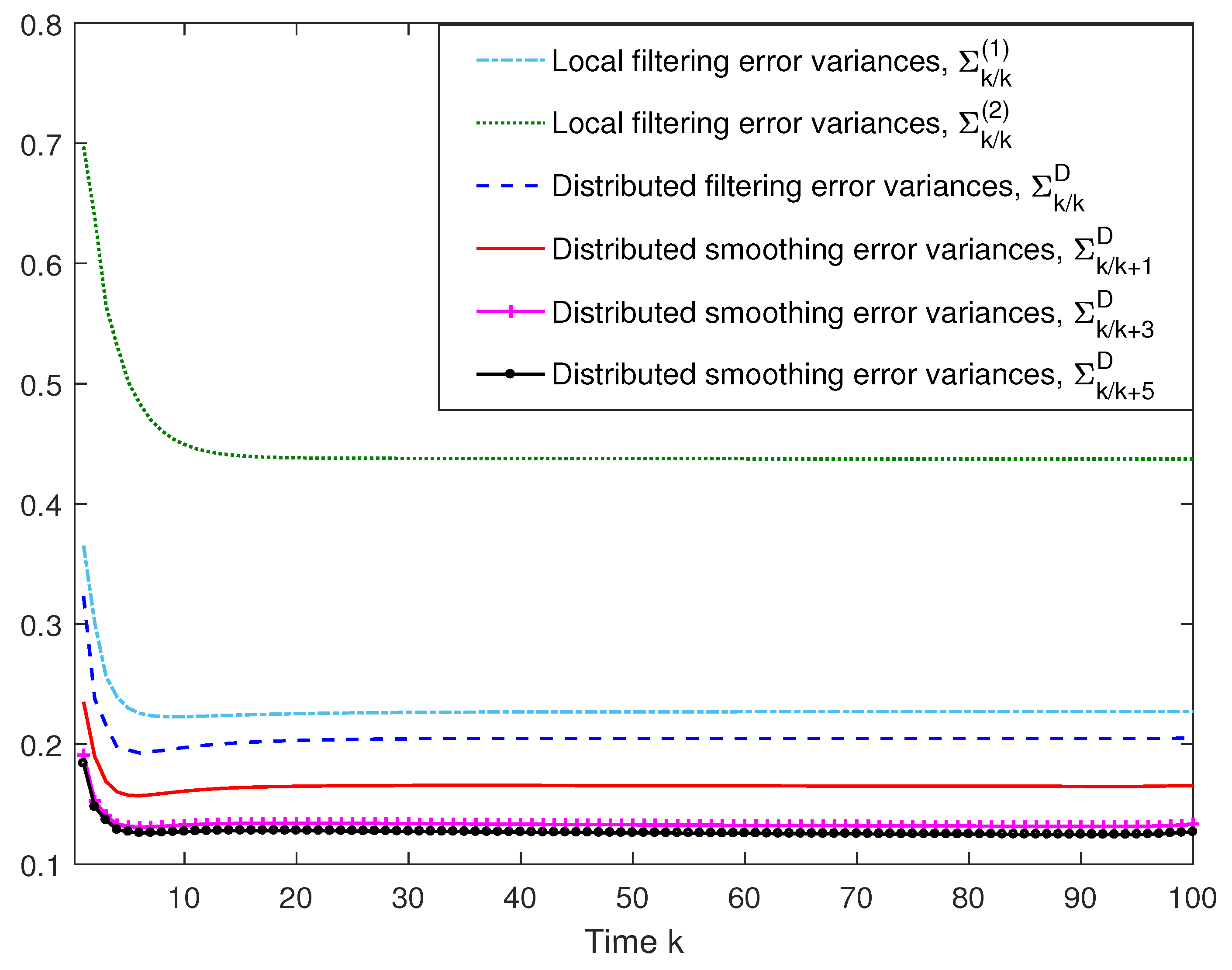
Figure 1 presents the local filtering error variances, Σ k / k ( i ) , i = 1 , 2 , and the distributed filtering and fixed-point smoothing error variances, Σ k / k + S D , S = 0 , 1 , 3 , 5 , and shows, on the one hand, that the distributed filtering error variances are lower than those of every local filter and, on the other, that the error variances corresponding to the distributed smoothers are smaller than those of the distributed filter. We conclude, therefore, that the smoothers are more accurate than the filter. Moreover, the distributed smoothing error variances at each fixed-point k decrease as the number of available measurements, k + S , increases, although the difference is almost insignificant for S > 5 .
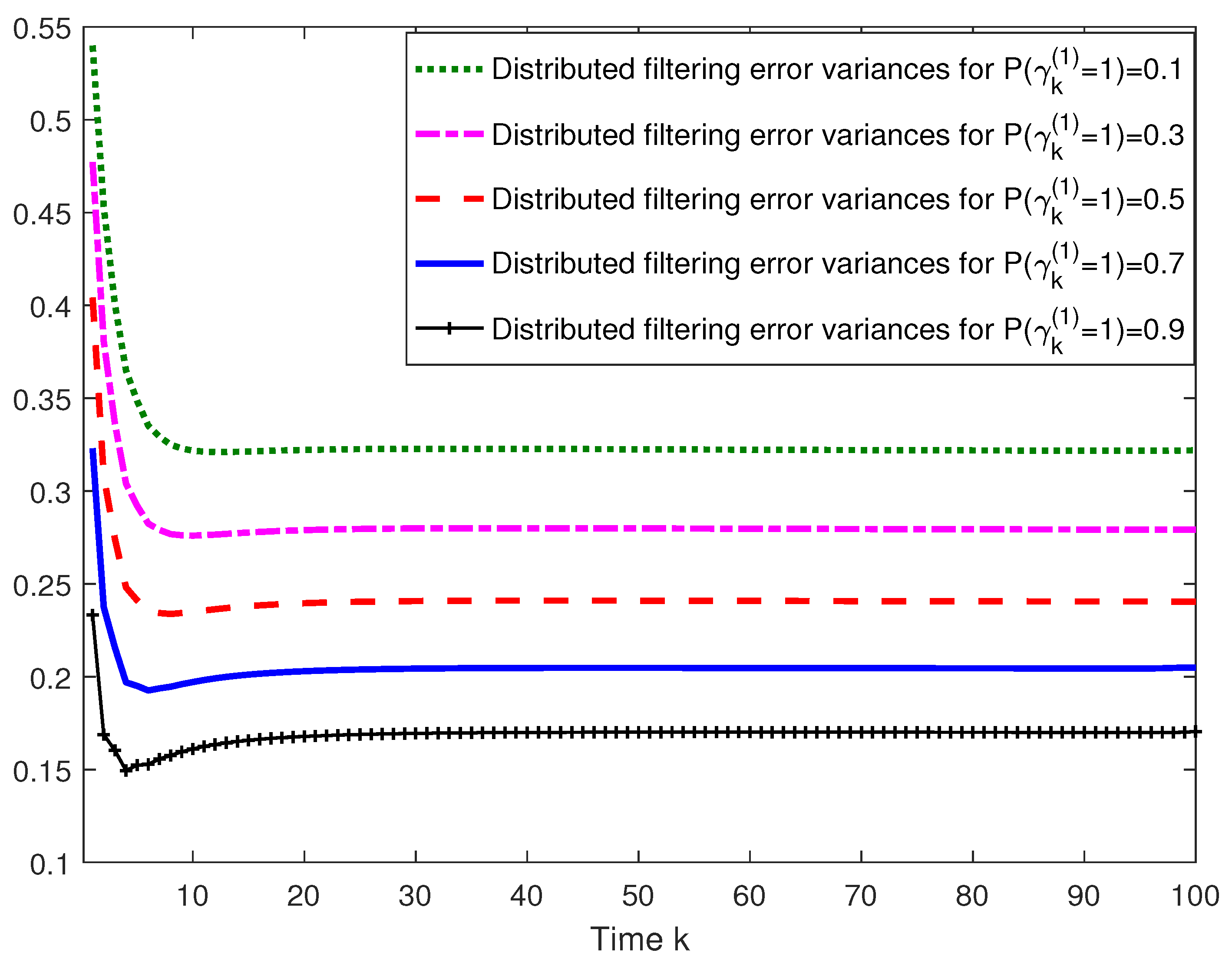
To determine the influence of estimator performance on sensor gain degradation, we calculated the distributed filtering error variances for different probability distributions of the random variables modelling the degradation. To do this, we set P γ k ( 1 ) = 0 = 0.1 and varied the probabilities of the values 0.5 and 1. Figure 2 shows that the filtering error variances decrease as P γ k ( 1 ) = 1 increases, thus confirming, as expected, that the distributed filtering performance improves when there is less signal degradation. An analogous study was conducted of the distributed smoothing error variances, from which similar conclusions were drawn.
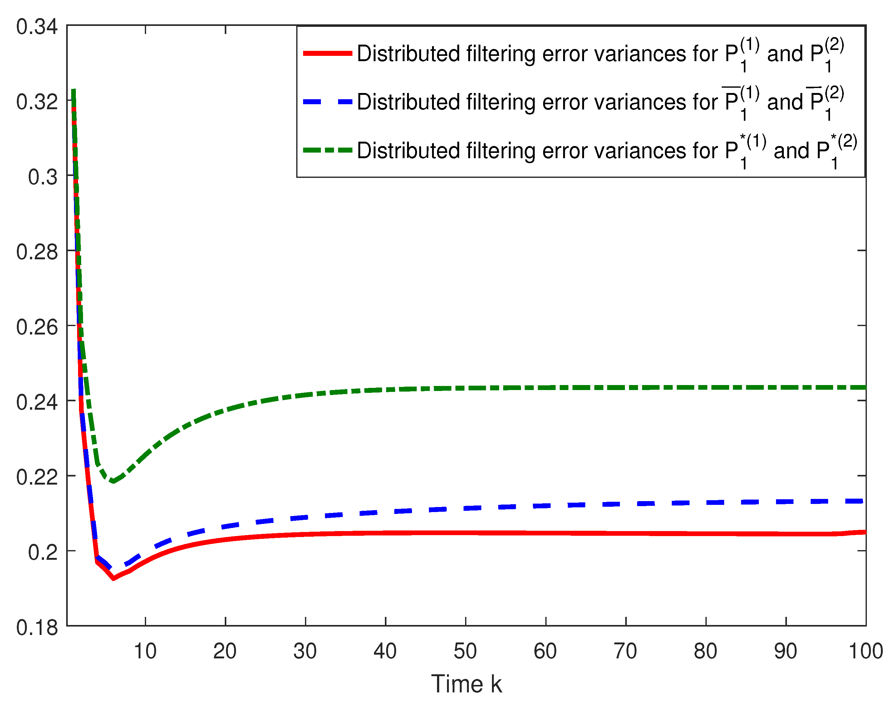
Next, we considered the use of various homogeneous Markov chains to model random delays in order to determine their influence on the accuracy of the proposed estimators. Concretely, we calculated the distributed filtering error variances, assuming that random delays can be appropriately modelled by homogeneous Markov chains with the same initial distribution and the following transition probability matrices: P 1 ( 1 ) , P 1 ( 2 ) ,
P ¯ 1 ( 1 ) = 0.99 0.002 0.008 0.001 0.98 0.019 0.08 0.04 0.88 , P ¯ 1 ( 2 ) = 0.99 0.001 0.009 0.001 0.98 0.019 0.062 0.058 0.88 ,
P 1 * ( 1 ) = 0.95 0.03 0.02 0.05 0.89 0.06 0.07 0.01 0.92 , P 1 * ( 2 ) = 0.89 0.07 0.04 0.055 0.89 0.055 0.08 0.04 0.88 .
The properties of the Markov chains lead us to conclude that the probabilities of no delay converge to the following constant values: 0.89, 0.77, 0.68, 0.60, 0.55 and 0.38 for P 1 ( 1 ) , P 1 ( 2 ) , P ¯ 1 ( 1 ) , P ¯ 1 ( 2 ) , P 1 * ( 1 ) and P 1 * ( 2 ) , respectively. Figure 3 shows the distributed filtering error variances for the different Markov chains considered. As expected, the performance of the distributed filtering estimators improved as the probabilities of no delay converged to higher values. Similar results were obtained for the smoothing error variances and, therefore, the same conclusions can be drawn for the distributed smoothers.
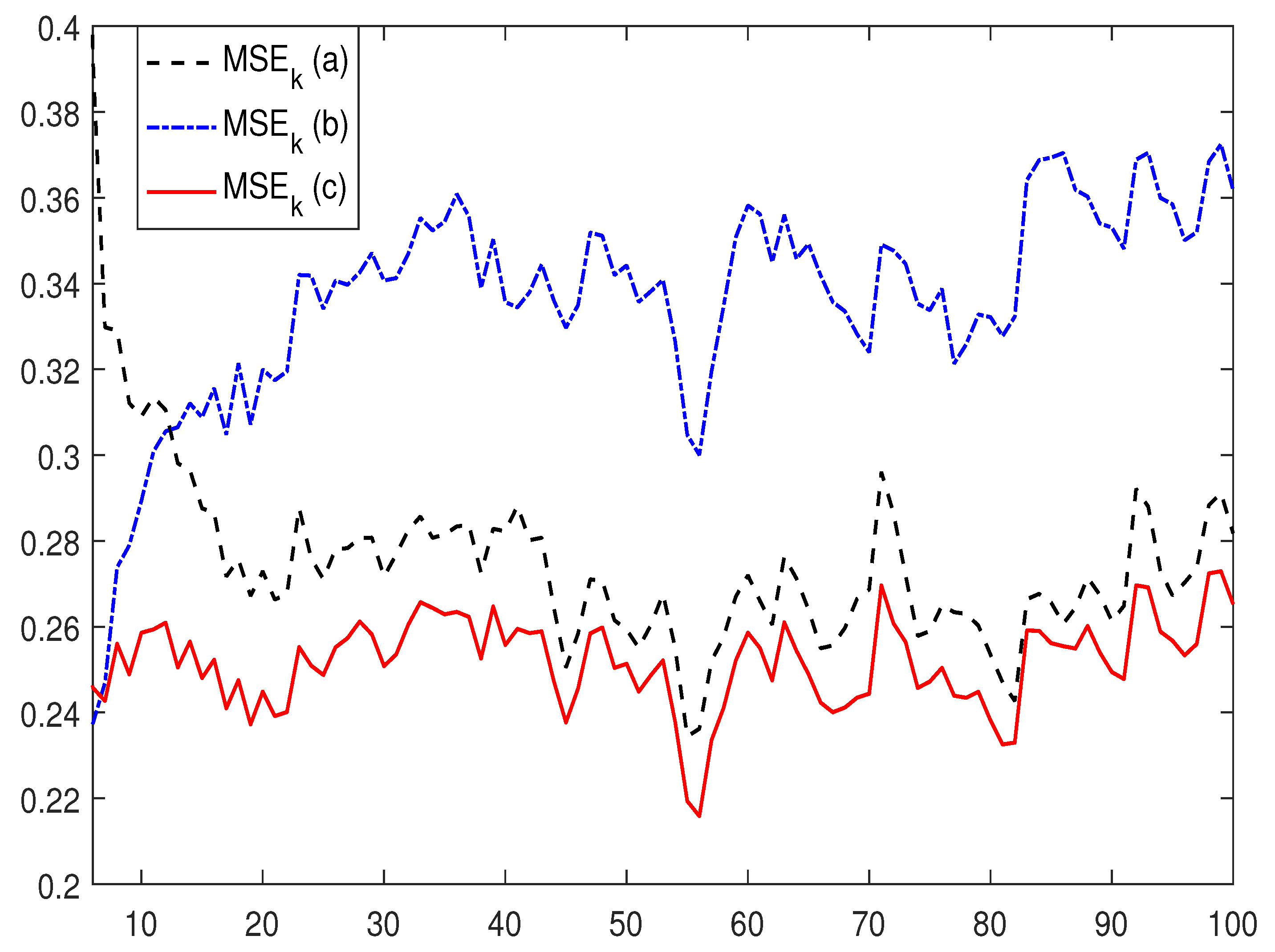
Finally, in order to show the performance of the proposed distributed filter, we conduct a comparative analysis between the proposed filter and ( a ) the distributed filter obtained in the model without gain degradation and independent white measurement noises, and ( b ) the distributed filter obtained when the delays during transmission are considered independent. To analyze the feasibility of the different distributed filters, the mean squared errors at each time instant k (MSE k ) of the different filters are calculated for 1000 independent simulations. Figure 4 shows that the MSE k for the proposed filter are less than for the other filters, which is due to the fact that these filters do not take into account all the hypotheses inherent to the model under study.

5. Conclusions

This paper describes how LS distributed fusion linear filter and fixed-point smoothers were derived for a class of discrete-time multi-sensors systems affected by stochastic sensor gain degradations, correlated measurement noises and one or two-step random transmission delays. The gain degradation in the different sensors is represented by independent white sequences of random variables with values in [0, 1], thus including the conventional missing signal phenomenon. The measurement noises are assumed to be correlated and cross-correlated at the same and at consecutive sampling times. The absence or presence of delays in the transmissions, due to the unreliability of the network, is described by different homogeneous discrete-time Markov chains. We address the distributed fusion estimation problem for networked systems with these characteristics, assuming that only the first and second-order moments of the processes involved in the observation model are available. Distributed filtering and fixed-point smoothing estimators are obtained as the LS matrix-weighted linear combination of the local ones. The filtering and fixed-point smoothing error variances, which are calculated offline, are used to measure accuracy of the proposed distributed estimators.
As indicated, in this paper we consider transmission delays described by different homogeneous discrete-time Markov chains. In Shang [34] two types of time delays are simultaneously considered; namely, signal transmission delays and signal processing delays. Hence, a challenging further research topic is to address the distributed estimation fusion problems considering these different types of delays.

Author Contributions

All authors contributed equally in deriving and implementing the proposed estimation algorithms and in writing this manuscript. All authors have read and agreed to the published version of the manuscript.

Funding

This research is supported by Ministerio de Economía, Industria y Competitividad, Agencia Estatal de Investigación and Fondo Europeo de Desarrollo Regional FEDER (grant no. MTM2017-84199-P).

Conflicts of Interest

The authors declare they have no conflict of interest.

Appendix A. Proof of Theorem 2

The proof is performed in the following four steps.
Derivation of (11) and (12).
Clearly, (11) is obtained from (3) for x ^ k / k ( i ) and r k d e ( i j ) = E O k d ( i ) O k e ( j ) T . Expression (12) for r k d e ( i j ) is derived by using (5) for O k d ( i ) and O k e ( j ) together with J k d ( i j ) = E [ O k d ( i ) μ k ( j ) T ] and J k 1 , k d ( i j ) = E [ O k 1 d ( i ) μ k ( j ) T ] .
Derivation of (13) and (14).
Expression (13) for J k 1 , k d ( i j ) = E O k 1 d ( i ) μ k ( j ) T is obtained by using (6) for the innovation, r k d y ( i j ) = E O k d ( i ) O k y ( j ) T , and denoting J k , k d ( i j ) = E O k d ( i ) μ k j T and D k , k 1 d ( i j ) = E y k ( i ) O k 1 d ( j ) T .
Expression (14) for J k , k d ( i j ) = E O k d ( i ) μ k ( j ) T is derived by using (5) for O k d ( i ) , taking into account that J k 1 , k d ( i j ) = E O k 1 d ( i ) μ k ( j ) T and that Π k , k ( i j ) = E μ k ( i ) μ k ( j ) T .
Derivation of (15)–(17).
To derive (15) for D k , k 1 d ( i j ) = E y k ( i ) O k 1 d ( j ) T , we first use (5) for O k 1 d ( j ) , and by denoting Y k , k 1 ( i j ) = E y k ( i ) μ k 1 ( j ) T , we obtain
D k , k 1 d ( i ) = ( 1 δ k , 2 ) E y k ( i ) O k 2 d ( j ) T + Y k , k 1 ( i j ) Π k 1 ( j ) 1 J k 1 d ( j ) T , k 2 .
Now, from (2) for y k ( i ) and the model hypotheses, we have
E y k ( i ) O k 2 d ( j ) T = a = 0 2 π k , a ( i ) γ ¯ k a ( i ) H k a ( i ) E x k a O k 2 d ( j ) T + a = 0 2 π k , a ( i ) E v k a ( i ) O k 2 d ( j ) T .
Taking into account that x ^ k a / k 2 ( j ) = A k a O k 2 d ( j ) , 0 a 2 (this expression for the signal predictor is obtained by a reasoning analogous to that carried out in García-Ligero et al. [24]), from the OPL we obtain E x k a O k 2 d ( j ) T = E x ^ k a / k 2 ( j ) O k 2 d ( j ) T = A k a r k 2 d ( j ) . Then, as v k ( i ) is uncorrelated with O k 2 d ( j ) , denoting V k , k d ( i j ) = E v k ( i ) O k d ( j ) T , we have
E y k ( i ) O k 2 d ( j ) T = a = 0 2 π k , a ( i ) γ ¯ k a ( i ) H k a ( i ) A k a r k 2 x d ( j ) + a = 1 2 π k , a ( i ) V k a , k 2 d ( i j ) , k 3 ,
and thus expression (15) is obtained.
From (5) for O k d ( i ) and denoting V k , k ( i j ) = E v k ( i ) μ k ( j ) T , it is clear that
V k , 1 d ( i j ) = V k , 1 ( i j ) Π 1 ( j ) 1 J 1 d ( j ) T , k = 1 , 2 , V k , k d ( i j ) = δ k , k E v k ( i ) O k 1 d ( j ) T + V k , k ( i j ) Π k ( j ) 1 J k d ( j ) T , k = k 1 , k ; k 2 .
Then, again using (5) for O k 1 d ( j ) and since E v k ( i ) O k 2 d ( j ) T = 0 , expression (16) is proven.
In order to obtain (17) for V k , k ( i j ) = E v k ( i ) μ k ( j ) T , first, we use (6) for the innovation, which leads us to
V k , k 1 ( i j ) = π k 1 , 0 ( j ) R k , k 1 ( i j ) , k 2 , V k , k ( i j ) = E v k ( i ) y k ( j ) T E v k ( i ) O k 1 y ( j ) T A k ( j ) T h = ( k 1 ) 1 k 1 V k , h ( i j ) Π h ( j ) 1 G k , h ( j ) T , k = k , k + 1 , k + 2 ; k 1 .
Next, we compute the two expectations in (A1):
From (2) for y k ( j ) and from assumptions 3 and 4, we obtain
E v k ( i ) y k ( j ) T = a = ( k k 1 ) 0 ( k k + 1 ) ( k 1 ) 2 π k , a ( j ) R k , k a ( i j ) , k = k , k + 1 , k + 2 ; k 1 .
Using (5) for O k 1 y ( j ) and again taking into account the independence of v k and O k 2 y ( j ) , we have
E v k ( i ) O k 1 y ( j ) T = h = ( k 1 ) 1 k 1 V k , h ( i j ) Π h ( j ) 1 J h y ( j ) T , k = k , k + 1 , k + 2 ; k 1 .
Expression (17) is then proven by substituting (A2) and (A3) in (A1).
Derivation (18) and (19).
From expression (6) for the innovation and denoting Y k , k ( i j ) = E y k ( i ) μ k ( j ) T , it is clear that
Π k , k ( i j ) = E ( y k ( i ) y ^ k / k 1 ( j ) ) μ k ( j ) T = Y k , k ( i j ) ( 1 δ k , 1 ) A k ( i ) E [ O k 1 y ( i ) μ k ( j ) T ] ( 1 δ k , 1 ) h = ( k 3 ) 1 k 1 G k , h ( i ) Π h ( i ) 1 E μ h ( i ) μ k ( j ) T .
Then, taking into account that J k , k y ( i j ) = E [ O k y ( i ) μ k ( j ) T ] and Π k , k ( i j ) = E [ μ k ( i ) μ k ( j ) T ] , we obtain (18).
Now, using (2) for y k ( i ) , the model assumptions and the fact that X k , k ( j ) = E x k μ k ( j ) T , it is clear that
Y k , k ( i j ) = E y k ( i ) μ k ( j ) T = a = 0 ( k 1 ) 2 π k , a ( i ) γ ¯ k a ( i ) H k a ( i ) X k a , k ( j ) + V k a , k ( i j ) , k , k 1 .
Then, taking into account that V k , k ( i j ) = 0 , k = k 3 , k 2 , (19) is obtained.

Appendix B. Proof of Theorem 3

Expression (20) for K k / S ( i j ) , S k + 1 , is readily obtained from (7) and Φ k , S ( i j ) = E x ^ k / S 1 ( i ) μ S ( j ) T .
For i = j , from the OPL, it is clear that Φ k , S ( i ) = 0 , S k . Next, we derived expression (21) for Φ k , S ( i j ) .
For S = k 1 , k , k + 1 , expression (21) of Φ k , S ( i j ) , is clear from (3) taking into account that J S 1 , S x ( i j ) = E O S 1 x ( i j ) μ S ( j ) T .
In order to calculate Φ k , S ( i j ) for S k + 2 , we use (7) for x ^ k / S 1 ( i ) , and from μ S ( j ) = y S ( j ) y ^ S / S 1 ( j ) , we obtain
Φ k , S ( i j ) = E x ^ k / S 2 ( i ) y S ( j ) T E x ^ k / S 2 ( i ) y ^ S / S 1 ( j ) T + X k , S 1 ( i ) Π S 1 ( i ) 1 Π S 1 , S ( i j ) .
To determine the first expectation in (A4), we use (2) for y S ( j ) and taking into account that by the OPL E x ^ k / S 2 ( i ) x S a T = E x ^ k / S 2 ( i ) x ^ S a / S 2 ( i ) T , we obtain
E x ^ k / S 2 ( i ) y S ( j ) T = a = 0 2 π S , a ( j ) γ ¯ S a ( j ) E x ^ k / S 2 ( i ) x ^ S a / S 2 ( i ) T H S a ( j ) T + a = 1 2 π S , a ( j ) E x ^ k / S 2 ( i ) v S a ( j ) T .
Now, expressing x ^ S a / S 2 ( i ) = A S a O k 2 x ( i ) in the first sum and using (7) for x ^ k / S 2 ( i ) in the second one, we have
E x ^ k / S 2 ( i ) y S ( j ) T = E k , S 2 x ( i ) H A S ( j ) T + π S , 2 ( j ) E x ^ k / S 3 ( i ) v S 2 ( j ) T + a = 1 2 π S , a ( j ) X k , S 2 ( i ) Π S 2 ( i ) 1 V S a , S 2 ( j i ) T ,
and, again, from (7) for x ^ k / S 3 ( i ) ,
E x ^ k / S 2 ( i ) y S ( j ) T = E k , S 2 x ( i ) H A S ( j ) T + ( 1 δ S , 3 ) π S , 2 ( j ) X k , S 3 ( i ) Π S 3 ( i ) 1 V S 2 , S 3 ( j i ) T + a = 1 2 π S , a ( j ) X k , S 2 ( i ) Π S 2 ( i ) 1 V S a , S 2 ( j i ) T .
To compute the second expectation in (A4), first, from (6), we write the observation predictor as
y ^ S / S 1 ( j ) T = A S ( j ) O S 1 y ( j ) ( 1 δ S , 1 ) h = ( S 3 ) 1 S 1 G S , h ( j ) Π h ( j ) 1 μ h ( j ) ;
then, expression (5) for O S 1 y ( j ) , together with Y S , S 1 ( j ) = A S ( j ) J S 1 y ( j ) T and E k , S y ( i j ) = E x ^ k / S ( i ) O S y ( j ) T , leads us to
E x ^ k / S 2 ( i ) y ^ S / S 1 ( j ) T = E k , S 2 y ( i j ) A S ( j ) T + Φ k , S 1 ( i j ) Π S 1 ( j ) 1 Y S , S 1 ( j ) T + h = ( S 3 ) 1 S 2 E x ^ k / S 2 ( i ) μ h ( j ) T Π h ( j ) 1 G S , h ( j ) T .
Again using expression (7) of the local smoother, after some manipulation, we obtain
E x ^ k / S 2 ( i ) y ^ S / S 1 ( j ) T = E k , S 2 y ( i j ) A S ( j ) T + Φ k , S 1 ( i j ) Π S 1 ( j ) 1 Y S , S 1 ( j ) T + h = ( S 3 ) 1 S 2 Φ k , h ( i j ) + h = h S 2 X k , h ( i ) Π h ( i ) 1 Π h , h ( i j ) Π h ( j ) 1 G S , h ( j ) T .
Substituting (A5) and (A6) in (A4), expression (21) for Φ k , S ( i j ) , S k + 2 , i j is proven.
Finally, expressions (22) and (23) of E k , S x ( i ) and E k , S y ( i j ) , S > k , are straightforwardly derived using (7) for x ^ k / S ( i ) and (5) for O S x ( i ) and O S y ( j ) , respectively. The initial conditions of both expressions are directly obtained from (3) and r k d e ( i j ) = E O k d ( i ) O k e ( j ) T .

References

  1. Ding, D.; Wang, Z.; Shen, B. Recent advances on distributed filtering for stochastic systems over sensor networks. Int. J. Gen. Syst. 2014, 43, 372–386. [Google Scholar] [CrossRef]
  2. Dong, H.; Wang, Z.; Ding, S.X.; Gao, H. A survey on distributed filtering and fault detection for sensor networks, Math. Probl. Eng. 2014, 2014, 858624. [Google Scholar] [CrossRef] [Green Version]
  3. Li, W.; Wang, Z.; Wei, G.; Ma, L.; Hu, J.; Ding, D. A survey on multisensor fusion and consensus filtering for sensor networks, Discret. Dyn. Nat. Soc. 2015, 2015, 683701. [Google Scholar] [CrossRef] [Green Version]
  4. Sun, S.L.; Lin, H.L.; Ma, J.; Li, X.Y. Multi-sensor distributed fusion estimation with applications in networked systems: A review paper. Inf. Fusion. 2017, 38, 122–134. [Google Scholar] [CrossRef]
  5. Yang, C.; Yang, Z.; Deng, Z. Robust weighted state fusion Kalman estimators for networked systems with mixed uncertainties. Inf. Fusion 2019, 45, 246–265. [Google Scholar] [CrossRef]
  6. Xia, J.; Gao, S.; Qi, X.; Zhanga, J.; Li, G. Distributed cubature H-infinity information filtering for target tracking against uncertain noise statistics. Signal Proccess. 2020, 177, 107725. [Google Scholar] [CrossRef]
  7. Hua, Z.; Hua, J.; Yanga, G. A survey on distributed filtering, estimation and fusion for nonlinear systems with communication constraints: New advances and prospects. Syst. Sci. Control. Eng. 2020, 8, 189–205. [Google Scholar] [CrossRef] [Green Version]
  8. Caballero-Águila, R.; García-Garrido, I.; Linares-Pérez, J. Information fusion algorithms for state estimation in multi-sensor systems with correlated missing measurements. Appl. Math. Comput. 2014, 226, 548–563. [Google Scholar] [CrossRef]
  9. Pang, C.; Sun, S. Fusion predictors for multi-sensor stochastic uncertain systems with missing measurements and unknown measurement disturbances. IEEE Sens. J. 2015, 15, 4346–4354. [Google Scholar] [CrossRef]
  10. García-Ligero, M.J.; Hermoso-Carazo, A.; Linares-Pérez, J. Distributed fusion estimation in networked systems with uncertain observations and Markovian random delays. Signal Process. 2015, 106, 114–122. [Google Scholar] [CrossRef]
  11. Liu, Y.; Wang, Z.; Zhou, D. Optimal filtering for networked systems with stochastic sensor gain degradation. Automatica 2014, 50, 1521–1525. [Google Scholar] [CrossRef]
  12. Liu, Y.; Wang, Z.; He, X.; Zhou, D.H. Minimum-variance recursive filtering over sensor with stochastic sensor gain degradation: Algorithms and performance analysis. IEEE Trans. Control. Net. Syst. 2016, 3, 265–274. [Google Scholar] [CrossRef] [Green Version]
  13. Liu, Y.; Wang, Z.; He, X.; Ghinea, G.; Alsaadi, F.E. A Resilient Approach to Distributed Filter Design for Time-Varying Systems Under Stochastic Nonlinearities and Sensor Degradation. IEEE Tans. Signal. Process. 2017, 65, 1300–1309. [Google Scholar] [CrossRef]
  14. Feng, J.; Zeng, M. Descriptor recursive estimation for multiple sensors with different delay rates. Int. J. Control. 2011, 84, 584–596. [Google Scholar] [CrossRef]
  15. Li, N.; Sun, S.; Ma, J. Multi-sensor distributed fusion filtering for networked systems with different delay and loss rates. Digit. Signal Process. 2014, 34, 29–38. [Google Scholar] [CrossRef]
  16. Chen, B.; Zhang, W.; Yu, L. Distributed fusion estimation with missing measurements, random transmission delays and packet dropouts. IEEE Trans. Automat. Control 2014, 59, 1961–1967. [Google Scholar] [CrossRef]
  17. Sun, S.; Xiao, W. Distributed fusion filter for networked stochastic uncertain systems with transmission delays and packet dropouts. Signal Process. 2017, 130, 268–278. [Google Scholar] [CrossRef]
  18. Caballero-Águila, R.; Hermoso-Carazo, A.; Linares-Pérez, J. Networked distributed fusion estimation under uncertain outputs with random transmission delays, packet losses and multi-packet processing. Signal Process. 2019, 156, 71–83. [Google Scholar] [CrossRef]
  19. Caballero-Ãguila, R.; Hermoso-Carazo, A.; Linares-Pérez, J. Networked Fusion Filtering from Outputs with Stochastic Uncertainties and Correlated Random Transmission Delays. Sensors 2016, 16, 847. [Google Scholar] [CrossRef] [Green Version]
  20. Caballero-Águila, R.; Hermoso-Carazo, A.; Linares-Pérez, J. Fusion estimation from multisensor observations with multiplicative noises and correlated random delays in transmission. Mathematics 2017, 5, 45. [Google Scholar] [CrossRef]
  21. Han, C.; Zhang, H. Linear optimal filtering for discrete-time systems with random jump delays. Signal Process. 2009, 89, 3097–3104. [Google Scholar] [CrossRef]
  22. Song, H.; Yu, L.; Zhang, W.A. H filtering of network-based systems with random delay. Signal Process. 2009, 89, 615–622. [Google Scholar] [CrossRef]
  23. Han, C.; Zhang, H.; Fu, M. Optimal filtering for networked systems with Markovian communication delays. Automatica. 2013, 49, 3097–3104. [Google Scholar] [CrossRef]
  24. García-Ligero M., J.; Hermoso-Carazo, A.; Linares-Pérez, J. Least-squares estimators for systems with stochastic sensor gain degradation, correlated measurement noises and delays in transmission modelled by Markov chains. Int. J. Syst. Sci. 2020, 51, 731–745. [Google Scholar] [CrossRef]
  25. Ge, X.; Han, Q.L.; Jiang, X. Distributed H filtering over sensor networks with heterogeneous Markovian coupling intercommunication delays. IET Contr. Theory Appl. 2014, 9, 82–90. [Google Scholar] [CrossRef]
  26. García-Ligero M., J.; Hermoso-Carazo, A.; Linares-Pérez, J. Distributed and centralized fusion estimation from multiple sensors with Markovian delays. Appl. Math. Comput. 2012, 219, 2932–2948. [Google Scholar] [CrossRef]
  27. Shang, Y. Couple-group consensus of continuous-time multi-agent systems under Markovian switching topologies. J. Frankl. Inst. 2015, 352, 4826–4844. [Google Scholar] [CrossRef]
  28. Shang, Y. Consensus seeking over Markovian switching networks with time-varying delays and uncertain topologies. Appl. Math. Comput. 2016, 273, 1234–1245. [Google Scholar] [CrossRef]
  29. Feng, J.; Wang, Z.; Zeng, M. Distributed weighted robust Kalman filter fusion for uncertain systems with autocorrelated and cross-correlated noises. Inf. Fusion. 2013, 14, 76–86. [Google Scholar] [CrossRef]
  30. Li, W.; Jia, Y.; Du, J. Distributed filtering for discrete-time linear systems with fading measurements and time-correlated noise. Digit. Signal Process. 2017, 60, 211–219. [Google Scholar] [CrossRef]
  31. Tian, T.; Sun, S.; Lin, H. Distributed fusion filter for multi-sensor systems with finite-step correlated noises. Inf. Fusion 2019, 46, 128–140. [Google Scholar] [CrossRef]
  32. Caballero-Águila, R.; Hermoso-Carazo, A.; Linares-Pérez, J. Least-Squares filtering algorithm in sensor networks with noise correlation and multiple random failures in transmission. Math. Probl. Eng. 2017, 2017, 1570719. [Google Scholar] [CrossRef] [Green Version]
  33. GarcÃa-Ligero, M.J.; Hermoso-Carazo, A.; Linares-Pérez, J. Estimation from a multisensor environment for systems with multiple packet dropouts and correlated measurement noises. Appl. Math. Model. 2017, 45, 324–332. [Google Scholar] [CrossRef]
  34. Shang, Y. On the Delayed Scaled Consensus Problems. Appl. Sci. 2017, 7, 713. [Google Scholar] [CrossRef] [Green Version]
Figure 1. Local filtering, distributed filtering and fixed-point smoothing error variances.
Mathematics 08 01948 g001
Figure 2. Distributed filtering error variances for different values of P γ k ( 1 ) = 1 .
Mathematics 08 01948 g002
Figure 3. Distributed filtering error variances for different transition probability matrices.
Mathematics 08 01948 g003
Figure 4. MSE k for distributed filter (a) for systems without gain degradation and independent white measurement noises, (b) for systems with independent delays and (c) for systems at hand.
Mathematics 08 01948 g004
Publisher’s Note: MDPI stays neutral with regard to jurisdictional claims in published maps and institutional affiliations.

