Solutions of Sturm-Liouville Problems

Abstract

This paper further improves the Lie group method with Magnus expansion proposed in a previous paper by the authors, to solve some types of direct singular Sturm–Liouville problems. Next, a concrete implementation to the inverse Sturm–Liouville problem algorithm proposed by Barcilon (1974) is provided. Furthermore, computational feasibility and applicability of this algorithm to solve inverse Sturm–Liouville problems of higher order (for $n=2,4$) are verified successfully. It is observed that the method is successful even in the presence of significant noise, provided that the assumptions of the algorithm are satisfied. In conclusion, this work provides a method that can be adapted successfully for solving a direct (regular/singular) or inverse Sturm–Liouville problem (SLP) of an arbitrary order with arbitrary boundary conditions.

1. Introduction

The inverse Sturm–Liouville theory was originated in 1929 by Ambarzumian [1] and further developed in [2,3,4,5,6].

The $2m$th order, nonsingular, self-adjoint eigenvalue problem (EVP) or Sturm–Liouville problem (SLP) is given by:

$$\begin{array}{c}{(-1)}^m{\left(p_0\left(x\right)y^{\left(m\right)}\right)}^{\left(m\right)}+{(-1)}^{m-1}{\left(p_1\left(x\right)y^{(m-1)}\right)}^{(m-1)}\hfill \\ +\dots +{\left(p_{m-2}\left(x\right)y^{″}\right)}^{″}-{\left(p_{m-1}\left(x\right)y^{\prime }\right)}^{\prime }+p_m\left(x\right)y=\lambda w\left(x\right)y,a<x<b\hfill \end{array}$$

(1)

together with some boundary conditions at a and b, the functions $p_k,(0\le k\le m)$, and $w\left(x\right)$ being continuous on the finite closed interval $[a,b]$, and $p_0$ having a continuous derivative. In the inverse SLP, the coefficient functions $p_k$, $(0\le k\le m)$ need to be reconstructed, given suitable valid spectral data.

For a discussion of analytical methods and numerical methods for inverse SLP, see [7,8], respectively. Iterative methods [9,10], Rayleigh–Ritz method [11], finite difference approximation [12], Quasi-Newton method [13], shooting method [14], interval Newton’s method [15], finite-difference method [16], boundary value methods [17,18,19,20], Numerov’s method  [21,22,23], least-squares functional  [24], generalized Rundell–Sacks algorithm [25,26], spectral mappings [27], Lie-group estimation method [28], Broyden method [29,30], decent flow methods [31], modified Numerov’s method [32], Newton-type method [33], Fourier–Legendre series [34], and  Chebyshev polynomials [35] are of particular importance among the existing methods to solve inverse SLP.

Numerical algorithms to solve the inverse fourth-order Sturm–Liouville problem (FSLP) are proposed in  [36,37,38].

In [39], authors implemented Barcilon [9]’s iterative algorithm to solve inverse SLPs successfully. The present paper extends the results for the case $m=2$ by considering the general-order inverse SLP algorithm as described in [36].

2. Materials and Methods

Inverse SLP Algorithm for the General Order

Setting $p_0\left(x\right),w\left(x\right)\equiv 1$ in (1) and taking the domain $[0,1]$, the EVP reads as:

$$\begin{array}{c}{\left(y^{\left(m\right)}\right)}^{\left(m\right)}-{\left(p_1{y}^{(m-1)}\right)}^{(m-1)}+\dots +p_m\left(x\right)y=\lambda y,0<x<1.\end{array}$$

(2)

According to [40], $m+1$ distinct spectra are required in order to determine $p_1\left(x\right),p_2\left(x\right),\dots ,p_m\left(x\right)$. In other words, $m+1$ different EVPs with distinct boundary conditions (BC) are needed. In addition, the spectra need to be interlaced, i.e.,

$$\begin{array}{c}\hfill \dots <{\lambda }_{n-1}^{(m+1)}<{\lambda }_n^{\left(1\right)}<{\lambda }_n^{\left(2\right)}<{\lambda }_n^{\left(3\right)}<\dots <{\lambda }_n^{(m+1)}<{\lambda }_{n+1}^{\left(1\right)}<\dots \end{array}$$

(3)

Assume that m boundary conditions are common to all the given $m+1$ eigenvalue problems, say, conditions at the right end point $x=1$.

• Combine the $m+1$ eigenvalue problems into an equivalent linear differential equation:

  1.1.

  Define a vector function $\mathit{\varphi }(x,\lambda )$:

  $$\begin{array}{cc}\hfill {\mathit{\varphi }}^T(x,\lambda )& =[\varpi \chi ,{\varpi }^{\prime }{\chi }^{\prime },\dots ,{\varpi }^{(m-1)}{\chi }^{(m-1)}]\hfill \\ \hfill & =[{\varphi }_{\left(1\right)},{\varphi }_{\left(2\right)},\dots ,{\varphi }_{\left(m\right)}]\hfill \end{array}$$

  where $\varpi (x,\lambda )$ and $\chi (x,\lambda )$ are two solutions of Equation (2).

  1.2.

  Differentiate each ${\varphi }_{\left(k\right)}$, $2m$ times.

  1.3.

  Obtain $m(2m+1)$ linear equations for ${\varpi }^{\left(i\right)}{\chi }^{\left(j\right)}+{\varpi }^{\left(j\right)}{\chi }^{\left(i\right)}$, where $i\le j$, $j=0,1,\dots ,2m-1$.

  1.4.

  Express ${\varpi }^{\left(i\right)}{\chi }^{\left(j\right)}+{\varpi }^{\left(j\right)}{\chi }^{\left(i\right)}$, $i\le j$, $j=0,1,\dots ,2m-1$, in terms of ${\varphi }_{\left(1\right)},{\varphi }_{\left(2\right)},\dots ,{\varphi }_{\left(m\right)}$ and their first $2m$ derivatives.

  1.5.

  Differentiate ${\varphi }_{\left(i\right)}^{\left(2m\right)}$, $i=1,2,\dots ,m$ again, to obtain m linear coupled differential equations of order $2m+1$, which is in matrix form:

  $$\begin{array}{cc}\hfill \mathcal{M}\mathit{\varphi }& =\lambda \mathcal{N}\mathit{\varphi }\hfill \end{array}$$

  (4)

• Obtain the corresponding boundary conditions for the linear differential equation using the boundary conditions of the $m+1$ eigenvalue problems:

  2.1.

  Assume that $\varpi (x,\lambda )$ and $\chi (x,\lambda )$ satisfy the m boundary conditions common to all the given $m+1$ eigenvalue problems.

  2.2.

  Then from 1.3, find the $m(3m+1)/2$ boundary conditions at $x=1$, and the $m(m+1)/2$ boundary conditions at $x=0$ for $\mathit{\varphi }(x,\lambda )$.

• Solve Equation (4) using above boundary conditions, to obtain the solutions ${\mathit{\varphi }}_n$.
• Solve the adjoint system of equations to the above system, and denote the solutions by ${\mathit{\eta }}_n$.
• Find the bi-orthogonal set of functions ${\left\{{\mathit{y}}_n\right\}}_1^{\infty }$ to ${\left\{{\mathit{\varphi }}_n\right\}}_1^{\infty }$, using the relation ${\mathit{y}}_n\left(x\right)={\mathcal{N}}^T{\mathit{\eta }}_n\left(x\right)$.

Some remarks on Algorithm 1 follow:

Line   (Data:)

Infinite eigenvalue (EV) sequence is replaced with the first N EVs. The truncated EV sequences ${\left\{{\lambda }_n^{\left(i\right)}\right\}}_{n=1}^N$, $i=1,2,\dots ,m+1$ are obtained, using the Magnus method [39] to solve Equation (2).

Line   (Result:)

Output $\mathbf{p}$: $m\times n$ matrix of function values, n: the number of subdivisions in the x-axis and m: the number of potentials.

Line   (1)

We take initial guess ${\mathbf{p}}^{\left(0\right)}$ as ${\mathbf{0}}_{m\times n}$.

Line (3)

while loop exit condition is replaced with a maximum number of iterations: $kMAX$ and in each iteration the condition ${\sum }_{n=1}^{(m+1)N}|{\widehat{\sigma }}_n-{\sigma }_n^{(k-1)}|<tol$ ($tol$: a fixed tolerance) is checked to exit the loop.

Line (4)

$\langle ·\rangle$ denotes the integration w.r.t. x from 0 to 1 and ${\mathbf{e}}^T=[1,0]$. ${\mathbf{y}}_n$ and ${\mathit{\varphi }}_n$ are kept fixed at ${\mathbf{y}}_0$ and ${\mathit{\varphi }}_0$, which are the solutions by setting $p_i=0$, $\forall i$. Solutions ${\mathbf{y}}_0$ and ${\mathit{\varphi }}_0$ are calculated using Mathematica [41]. Matlab [42] built-in functions: trapz() and griddedInterpolant() with pchip (piecewise cubic Hermite interpolating polynomial) option are used to approximate integrals and to have p as a function, respectively. The latter is required since, p as a function is input to the Magnus method. Again, the eigenvalue sequence ${\sigma }^{\left(k\right)}$ is calculated using ${\mathbf{p}}^{\left(k\right)}$ and the iteration repeats.

You may refer Section 2.6 of [39] for the specific computational details of the Algorithm 1 for the case $m=1$ and next section for the case $m=2$.

Algorithm 1: Solving inverse Sturm–Liouville problem (SLP).

3. Inverse FSLP Algorithm

Setting $m=2$ in Equation (2) we obtain FSLP:

$$\begin{array}{cc}\hfill \mathcal{L}u& \equiv u^{\left(4\right)}-{\left(p{u}^{\prime }\right)}^{\prime }+qu=\lambda u.\hfill \end{array}$$

(8)

Three spectra $\left\{{\lambda }_n\right\}$, $\left\{{\mu }_n\right\}$ and $\left\{{\nu }_n\right\}$ required to reconstruct the unknown coefficients: p and q will be obtained from the following EVPs:

$$\begin{array}{cc}\hfill \mathcal{L}{u}_n={\lambda }_n{u}_n,& u_n\left(0\right)=u_n^{″}\left(0\right)=u_n\left(1\right)=u_n^{″}\left(1\right)=0,\hfill \end{array}$$

(9)

$$\begin{array}{cc}\hfill \mathcal{L}{v}_n={\mu }_n{v}_n,& v_n\left(0\right)=v_n^{\prime }\left(0\right)=v_n\left(1\right)=v_n^{″}\left(1\right)=0,\hfill \end{array}$$

(10)

$$\begin{array}{cc}\hfill \mathcal{L}{w}_n={\nu }_n{w}_n,& w_n^{\prime }\left(0\right)=w_n^{″}\left(0\right)=w_n\left(1\right)=w_n^{″}\left(1\right)=0.\hfill \end{array}$$

(11)

Although, Equations (9) and (10) are self-adjoint, Equation (11) is not. Its adjoint equation is:

$$\begin{array}{cc}\hfill \mathcal{L}{\omega }_n={\nu }_n{\omega }_n,& {\omega }_n^{\prime }\left(0\right)={\omega }_n^{‴}\left(0\right)-p\left(0\right){\omega }_n^{\prime }\left(0\right)={\omega }_n\left(1\right)={\omega }_n^{″}\left(1\right)=0.\hfill \end{array}$$

(12)

The eigenvalues ${\lambda }_n$, ${\mu }_n$ and ${\nu }_n$ (for $p=q=0$) are given by the solutions of the following equations:

$$\begin{array}{cc}\hfill sin\left(s\right)& =0,s^4=\lambda \hfill \end{array}$$

(13)

$$\begin{array}{cc}\hfill tan\left(r\right)-tanh\left(r\right)& =0,r^4=\mu \hfill \end{array}$$

(14)

$$\begin{array}{cc}\hfill tan\left(t\right)+tanh\left(t\right)& =0,t^4=\nu \hfill \end{array}$$

(15)

Furthermore,

$$\begin{array}{cc}\hfill t\approx \left(n-\frac{1}{4}\right)\pi ,s=n\pi ,r\approx \left(n+\frac{1}{4}\right)\pi ,& n\in \mathbb{N}\hfill \end{array}$$

so that the spectra $\left\{{\lambda }_n\right\}$, $\left\{{\mu }_n\right\}$ and $\left\{{\nu }_n\right\}$ are interlaced, i.e.,

$$0<{\nu }_1<{\lambda }_1<{\mu }_1<{\nu }_2<{\lambda }_2<{\mu }_2<\dots$$

Since the eigenvalues are interlaced, they can be coalesced into a single one by defining

$$\begin{array}{cc}\hfill {\left\{{\sigma }_k,\left[\begin{array}{c}{\varphi }_k\\ {\psi }_k\end{array}\right]\right\}}_1^{\infty }& =\left\{\begin{array}{cc}{\left\{{\nu }_n,\left[\begin{array}{c}{w}_n{\omega }_n\\ w_n^{\prime }{\omega }_n^{\prime }\end{array}\right]\right\}}_1^{\infty }\hfill & \mathrm{for}k=3n-2,\hfill \\ {\left\{{\lambda }_n,\left[\begin{array}{c}{u}_n^2\\ u_n^{{}^{\prime }2}\end{array}\right]\right\}}_1^{\infty }\hfill & \mathrm{for}k=3n-1,\hfill \\ {\left\{{\mu }_n,\left[\begin{array}{c}{v}_n^2\\ v_n^{{}^{\prime }2}\end{array}\right]\right\}}_1^{\infty }\hfill & \mathrm{for}k=3n,\hfill \end{array}\right.n=1,2,\dots .\hfill \end{array}$$

(16)

Denote:

$$\begin{array}{cc}\hfill \mathbf{q}=\left[\begin{array}{c}q\\ p\end{array}\right],& {\mathit{\varphi }}_n=\left[\begin{array}{c}{\varphi }_n\\ {\psi }_n\end{array}\right].\hfill \end{array}$$

(17)

Let $\chi (x,\lambda )$ and $\varpi (x,\lambda )$ be two solutions of (8) satisfying the common boundary conditions of Equations (9)–(12), namely, ($u\left(1\right)=u^{″}\left(1\right)=0$, etc.)

$$\begin{array}{cc}\hfill \chi (1,\lambda )& =\varpi (1,\lambda )={\chi }^{″}(1,\lambda )={\varpi }^{″}(1,\lambda )=0.\hfill \end{array}$$

(18)

Guided by (16), define

$$\begin{array}{c}\hfill \left\{\begin{array}{cc}\varphi (x,\lambda )=\varpi (x,\lambda )\chi (x,\lambda )\hfill & \\ \psi (x,\lambda )={\varpi }^{\prime }(x,\lambda ){\chi }^{\prime }(x,\lambda ).\hfill \end{array}\right.\end{array}$$

(19)

By differentiating $\varphi$ and $\psi$ five times each, and eliminating $\varpi$, and $\chi$, 9th order linear differential equation for $\varphi$ (or a coupled system of linear differential equations of order 5 for $\varphi$ and $\psi$) can be obtained. When $p=q=0$, this reduces to

$$\begin{array}{cc}\hfill {\varphi }^{\left(9\right)}\left(x\right)-12\lambda {\varphi }^{\left(5\right)}\left(x\right)& =64{\lambda }^2{\varphi }^{\left(1\right)}\left(x\right)\hfill \end{array}$$

(20)

or

$$\begin{array}{cc}\hfill \left(\begin{array}{cc}3D^5& -10D^3\\ 0& D^5\end{array}\right)\left(\begin{array}{c}\varphi \\ \psi \end{array}\right)& =\lambda \left(\begin{array}{cc}8D& 0\\ 10D^3& -24D\end{array}\right)\left(\begin{array}{c}\varphi \\ \psi \end{array}\right)\hfill \end{array}$$

(21)

in the form of the Equation (4), and the boundary conditions read as:

$$\begin{array}{cc}\hfill \varphi ={\varphi }^{‴}={\psi }^{\prime }=0& \mathrm{at}x=0,\hfill \end{array}$$

(22)

$$\begin{array}{cc}\hfill \varphi ={\varphi }^{\prime }={\varphi }^{″}-2\psi ={\varphi }^{‴}={\varphi }^{⁗}-4{\psi }^{″}={\psi }^{\prime }={\psi }^{‴}=0& \mathrm{at}x=1.\hfill \end{array}$$

(23)

The solution of the system of Equations (21)–(23) using Mathematica is:

$$\begin{array}{cc}\hfill \varphi \left(x\right)& =\frac{csc\left(\mu \right)}{8(2cosh(\mu )+cosh(2\mu \left)\right(-3cos\left(\mu \right)+cos\left(3\mu \right)-cos\left(\right(2+i\left)\mu \right)+cos\left(\right(1+2i\left)\mu \right)+cosh\left(\right(2+i\left)\mu \right)-cosh\left(\right(1+2i\left)\mu \right)\left)\right)}\hfill \\ \hfill & \times (icos((1+i)\left(\right(1+i)x+1)\mu )-icos((1+i)\left(\right(1+i)x\mu +\mu ))+16sin(2\mu )-4sin(4\mu )-(10+10i)sin((1+i)\mu )\hfill \\ \hfill & +(2-2i)sin\left(\right(3+i\left)\mu \right)-(4+4i)sin\left(\right(2+2i\left)\mu \right)-(2-2i)sin\left(\right(1+3i\left)\mu \right)+(2+2i)sin\left(\right(3+3i\left)\mu \right)\hfill \\ \hfill & -2isin\left(\right(1+i\left)\right((3+i)-x\left)\mu \right)-(6+6i)sin\left(\right(1+i\left)\right(x-2\left)\mu \right)+(2+2i)sin\left(\right(1+i\left)\right(x+2\left)\mu \right)\hfill \\ \hfill & +6isin\left(\right(1+i\left)\right((-1-i)+x\left)\mu \right)+2sin\left(\right(1+i\left)\right((-3+i)+x\left)\mu \right)+4sin\left(\right(1+i\left)\right(-2i+x\left)\mu \right)+4isin\left(\right(1+i\left)\right(2i+x\left)\mu \right)\hfill \\ \hfill & -(2+4i)sin\left(\right(1+i\left)\right((1+i)+x\left)\mu \right)-2isin\left(\right(1+i\left)\right((-1+3i)+x\left)\mu \right)+(2-2i)sin\left(\right(1+i\left)\right((-2-2i)+x\left)\mu \right)\hfill \\ \hfill & -2sin\left(\right(1+i\left)\right((-1-3i)+x\left)\mu \right)+2isin\left(\right((1+i)+2x\left)\mu \right)-2isin\left(\right((1+3i)+2x\left)\mu \right)-6isin\left(\right(2i+(1-i)x\left)\mu \right)\hfill \\ \hfill & +(2+2i)sin\left(\right(4i+(1-i)x\left)\mu \right)-2sin\left(\right((2+4i)+(1-i)x\left)\mu \right)+2sin\left(2\right(ix+1\left)\mu \right)+4isin\left(\right(1+i\left)\right(ix+2\left)\mu \right)\hfill \\ \hfill & +8sin\left(\right((1-i)+2ix\left)\mu \right)-2sin\left(\right((3+i)+2ix\left)\mu \right)+2sin\left(\right((1-3i)+2ix\left)\mu \right)-2sin\left(\right((3-3i)+2ix\left)\mu \right)\hfill \\ \hfill & +sin\left(\right(1+i\left)\right((1+i)x+1\left)\mu \right)-(4+2i)sin\left(\right((1+i)x+2\left)\mu \right)+8isin\left(\right((1+i)-2x\left)\mu \right)+2isin\left(\right((3+i)-2x\left)\mu \right)\hfill \\ \hfill & -2isin\left(\right((3+3i)-2x\left)\mu \right)-6sin\left(\right(2-(1-i)x\left)\mu \right)+(2+2i)sin\left(\right(4-(1-i)x\left)\mu \right)+2sin\left(2\right(1-ix\left)\mu \right)\hfill \\ \hfill & +4sin\left(\right(1+i\left)\right(2-ix\left)\mu \right)-8sin\left(2\right((1+i)-ix\left)\mu \right)+2sin\left(2\right((2+i)-ix\left)\mu \right)+2sin\left(2\right((1+2i)-ix\left)\mu \right)\hfill \\ \hfill & +2sin\left(\right((1-i)-2ix\left)\mu \right)-2sin\left(\right((3-i)-2ix\left)\mu \right)+8sin\left(\right((1+i)-2ix\left)\mu \right)+2sin\left(\right((1+3i)-2ix\left)\mu \right)\hfill \\ \hfill & -2sin\left(\right((3+3i)-2ix\left)\mu \right)-6sin\left(\right(2-(1+i)x\left)\mu \right)+(2-2i)sin\left(\right(4-(1+i)x\left)\mu \right)-(4-2i)sin\left(\right(1-i)x\mu \hfill \\ \hfill & +2\mu )+sin((1+i)\left(\right(1+i)x\mu +\mu ))-8isin((2+2i)\mu -2x\mu )+2isin((4+2i)\mu -2x\mu )\hfill \\ \hfill & +2isin\left(\right(2+4i)\mu -2x\mu )-16sinh\left(2\mu \right)+4sinh\left(4\mu \right)+(10+10i)sinh\left(\right(1+i\left)\mu \right)\hfill \\ \hfill & -(2-2i)sinh\left(\right(3+i\left)\mu \right)+(4+4i)sinh\left(\right(2+2i\left)\mu \right)+(2-2i)sinh\left(\right(1+3i\left)\mu \right)-(2+2i)sinh\left(\right(3+3i\left)\mu \right)\hfill \\ \hfill & +(6+6i)sinh\left(\right(1+i\left)\right(x-2\left)\mu \right)-(2+2i)sinh\left(\right(1+i\left)\right(x+2\left)\mu \right)-2isinh\left(\right(1+i\left)\right((-3-i)+x\left)\mu \right)+2isinh\left(2\right((-2-i)+x\left)\mu \right)\hfill \\ \hfill & -8isinh\left(2\right((-1-i)+x\left)\mu \right)-2sinh\left(\right(1+i\left)\right((-3+i)+x\left)\mu \right)+2isinh\left(2\right((-1-2i)+x\left)\mu \right)+2sinh\left(\right(1+i\left)\right((-1-3i)+x\left)\mu \right)\hfill \\ \hfill & -2sinh\left(2\right(ix+1\left)\mu \right)+2sinh\left(\right((3+i)+2ix\left)\mu \right)-2sinh\left(\right(1+i\left)\right((1+i)x+1\left)\mu \right)+(4+2i)sinh\left(\right((1+i)x+2\left)\mu \right)\hfill \\ \hfill & -2sinh\left(2\right(1-ix\left)\mu \right)+8sinh\left(2\right((1+i)-ix\left)\mu \right)-2sinh\left(2\right((2+i)-ix\left)\mu \right)-2sinh\left(2\right((1+2i)-ix\left)\mu \right)\hfill \\ \hfill & -8sinh\left(\right((1+i)-2ix\left)\mu \right)-2sinh\left(\right((1+3i)-2ix\left)\mu \right)+2sinh\left(\right((3+3i)-2ix\left)\mu \right))\hfill \end{array}$$

$$\begin{array}{cc}\hfill \psi \left(x\right)& =\frac{{\mu }^{2}csc\left(\mu \right)}{8(2cosh(\mu )+cosh(2\mu \left)\right(-3cos\left(\mu \right)+cos\left(3\mu \right)-cos\left(\right(2+i\left)\mu \right)+cos\left(\right(1+2i\left)\mu \right)+cosh\left(\right(2+i\left)\mu \right)-cosh\left(\right(1+2i\left)\mu \right)\left)\right)}\hfill \\ \hfill & \times (icos((1+i)\left(\right(1+i)x+1)\mu )-icos((1+i)\left(\right(1+i)x\mu +\mu ))-16sin(2\mu )+4sin(4\mu )+(10-10i)sin((1+i)\mu )\hfill \\ \hfill & -(2+2i)sin\left(\right(3+i\left)\mu \right)+(4-4i)sin\left(\right(2+2i\left)\mu \right)+(2+2i)sin\left(\right(1+3i\left)\mu \right)-(2-2i)sin\left(\right(3+3i\left)\mu \right)\hfill \\ \hfill & -2sin\left(\right(1+i\left)\right((3+i)-x\left)\mu \right)-(6-6i)sin\left(\right(1+i\left)\right(x-2\left)\mu \right)+(2-2i)sin\left(\right(1+i\left)\right(x+2\left)\mu \right)+6sin\left(\right(1+i\left)\right((-1-i)+x\left)\mu \right)\hfill \\ \hfill & -2isin\left(\right(1+i\left)\right((-3+i)+x\left)\mu \right)-4isin\left(\right(1+i\left)\right(-2i+x\left)\mu \right)+4sin\left(\right(1+i\left)\right(2i+x\left)\mu \right)-(4-2i)sin\left(\right(1+i\left)\right((1+i)+x\left)\mu \right)\hfill \\ \hfill & -2sin\left(\right(1+i\left)\right((-1+3i)+x\left)\mu \right)-(2+2i)sin\left(\right(1+i\left)\right((-2-2i)+x\left)\mu \right)+2isin\left(\right(1+i\left)\right((-1-3i)+x\left)\mu \right)-2isin\left(\right((1+i)+2x\left)\mu \right)\hfill \\ \hfill & +2isin\left(\right((1+3i)+2x\left)\mu \right)+6sin\left(\right(2i+(1-i)x\left)\mu \right)-(2-2i)sin\left(\right(4i+(1-i)x\left)\mu \right)-2isin\left(\right((2+4i)+(1-i)x\left)\mu \right)\hfill \\ \hfill & +2sin\left(2\right(ix+1\left)\mu \right)-4sin\left(\right(1+i\left)\right(ix+2\left)\mu \right)+8sin\left(\right((1-i)+2ix\left)\mu \right)-2sin\left(\right((3+i)+2ix\left)\mu \right)+2sin\left(\right((1-3i)+2ix\left)\mu \right)\hfill \\ \hfill & -2sin\left(\right((3-3i)+2ix\left)\mu \right)+sin\left(\right(1+i\left)\right((1+i)x+1\left)\mu \right)-(2-4i)sin\left(\right((1+i)x+2\left)\mu \right)-8isin\left(\right((1+i)-2x\left)\mu \right)\hfill \\ \hfill & -2isin\left(\right((3+i)-2x\left)\mu \right)+2isin\left(\right((3+3i)-2x\left)\mu \right)-6isin\left(\right(2-(1-i)x\left)\mu \right)-(2-2i)sin\left(\right(4-(1-i)x\left)\mu \right)+2sin\left(2\right(1-ix\left)\mu \right)\hfill \\ \hfill & +4isin\left(\right(1+i\left)\right(2-ix\left)\mu \right)-8sin\left(2\right((1+i)-ix\left)\mu \right)+2sin\left(2\right((2+i)-ix\left)\mu \right)+2sin\left(2\right((1+2i)-ix\left)\mu \right)+2sin\left(\right((1-i)-2ix\left)\mu \right)\hfill \\ \hfill & -2sin\left(\right((3-i)-2ix\left)\mu \right)+8sin\left(\right((1+i)-2ix\left)\mu \right)+2sin\left(\right((1+3i)-2ix\left)\mu \right)-2sin\left(\right((3+3i)-2ix\left)\mu \right)+6isin\left(\right(2-(1+i)x\left)\mu \right)\hfill \\ \hfill & -(2+2i)sin\left(\right(4-(1+i)x\left)\mu \right)-(2+4i)sin\left(\right(1-i)x\mu +2\mu )+sin\left(\right(1+i\left)\right((1+i)x\mu +\mu \left)\right)+8isin\left(\right(2+2i)\mu -2x\mu )\hfill \\ \hfill & -2isin\left(\right(4+2i)\mu -2x\mu )-2isin\left(\right(2+4i)\mu -2x\mu )-16sinh\left(2\mu \right)+4sinh\left(4\mu \right)+(10-10i)sinh\left(\right(1+i\left)\mu \right)\hfill \\ \hfill & -(2+2i)sinh\left(\right(3+i\left)\mu \right)+(4-4i)sinh\left(\right(2+2i\left)\mu \right)+(2+2i)sinh\left(\right(1+3i\left)\mu \right)-(2-2i)sinh\left(\right(3+3i\left)\mu \right)-(6-6i)sinh\left(\right(1+i\left)\right(x-2\left)\mu \right)\hfill \\ \hfill & +(2-2i)sinh\left(\right(1+i\left)\right(x+2\left)\mu \right)+2sinh\left(\right(1+i\left)\right((-3-i)+x\left)\mu \right)+2isinh\left(2\right((-2-i)+x\left)\mu \right)-8isinh\left(2\right((-1-i)+x\left)\mu \right)\hfill \\ \hfill & -2isinh\left(\right(1+i\left)\right((-3+i)+x\left)\mu \right)+2isinh\left(2\right((-1-2i)+x\left)\mu \right)+2isinh\left(\right(1+i\left)\right((-1-3i)+x\left)\mu \right)+2sinh\left(2\right(ix+1\left)\mu \right)\hfill \\ \hfill & -2sinh\left(\right((3+i)+2ix\left)\mu \right)+2sinh\left(\right(1+i\left)\right((1+i)x+1\left)\mu \right)-(2-4i)sinh\left(\right((1+i)x+2\left)\mu \right)+2sinh\left(2\right(1-ix\left)\mu \right)\hfill \\ \hfill & -8sinh\left(2\right((1+i)-ix\left)\mu \right)+2sinh\left(2\right((2+i)-ix\left)\mu \right)+2sinh\left(2\right((1+2i)-ix\left)\mu \right)+8sinh\left(\right((1+i)-2ix\left)\mu \right)+2sinh\left(\right((1+3i)-2ix\left)\mu \right)\hfill \\ \hfill & -2sinh\left(\right((3+3i)-2ix\left)\mu \right))\hfill \end{array}$$

with ${\mu }^4=\lambda$. The adjoint of system of Equations (21)–(23) is

$$\begin{array}{cc}\hfill \left(\begin{array}{cc}3D^5& 0\\ -10D^3& D^5\end{array}\right)\left(\begin{array}{c}\eta \\ \zeta \end{array}\right)& =\lambda \left(\begin{array}{cc}8D& 10D^3\\ 0& -24D\end{array}\right)\left(\begin{array}{c}\eta \\ \zeta \end{array}\right)\hfill \end{array}$$

(24)

with

$$\begin{array}{cc}\hfill \eta ={\eta }^{″}={\eta }^{‴}=\zeta ={\zeta }^{\prime }={\zeta }^{″}={\zeta }^{⁗}=0& \mathrm{at}x=0,\hfill \end{array}$$

(25)

$$\begin{array}{cc}\hfill \zeta ={\zeta }^{″}+2\eta ={\zeta }^{⁗}-4{\eta }^{″}=0& \mathrm{at}x=1.\hfill \end{array}$$

(26)

The solutions are

$$\begin{array}{cc}\hfill \eta \left(x\right)& =cos\left(2\mu x\right)+2cos\left(\right(1+i\left)\mu x\right)+cosh\left(2\mu x\right)+2cosh\left(\right(1+i\left)\mu x\right)\hfill \\ \hfill & +\frac{(2-2i)(sin(\mu )-sinh(\mu \left)\right)(sin(\mu )sinh(2\mu )-sin(2\mu )sinh(\mu \left)\right)}{(sin(2\mu )+sinh(2\mu \left)\right)(sin(\mu )cosh(\mu )-cos(\mu )sinh(\mu \left)\right)}(sin\left((1+i)\mu x\right)+sinh\left((1+i)\mu x\right))\hfill \\ \hfill & -\frac{(cos(2\mu )+cosh(2\mu )-2)}{sin\left(2\mu \right)+sinh\left(2\mu \right)}(sin\left(2\mu x\right)+sinh\left(2\mu x\right))-6\hfill \end{array}$$

$$\begin{array}{cc}\hfill \zeta \left(x\right)& =\frac{1}{{\mu }^2}(-cos\left(2\mu x\right)-2icos\left(\right(1+i\left)\mu x\right)+cosh\left(2\mu x\right)+2icosh\left(\right(1+i\left)\mu x\right)\hfill \\ \hfill & +\frac{(2+2i)(sin(\mu )-sinh(\mu \left)\right)(sin(\mu )sinh(2\mu )-sin(2\mu )sinh(\mu \left)\right)}{(sin(2\mu )+sinh(2\mu \left)\right)(sin(\mu )cosh(\mu )-cos(\mu )sinh(\mu \left)\right)}(sinh\left((1+i)\mu x\right)-sin\left((1+i)\mu x\right))\hfill \\ \hfill & \left.+\frac{(cos(2\mu )+cosh(2\mu )-2)}{sin\left(2\mu \right)+sinh\left(2\mu \right)}(sin\left(2\mu x\right)-sinh\left(2\mu x\right))\right).\hfill \end{array}$$

The bi-orthogonal set for $\left\{\mathit{\varphi }\right\}$ given by $\mathbf{y}={\mathcal{N}}^T\mathit{\eta }$ is:

$$\begin{array}{cc}\hfill y\left(x\right)& =\frac{24(1+i)\mu }{(sin(2\mu )+sinh(2\mu \left)\right)(sin(\mu )cosh(\mu )-cos(\mu )sinh(\mu \left)\right)}\hfill \\ \hfill & \times \left(-(2-2i){sin}^2\left(\mu \right)sinh\left(2\mu \right)cos\left(\mu x\right)cosh\left(\mu x\right)\right.\hfill \\ \hfill & +cos\left(\mu \right)sinh\left(\mu \right)\left(-sin\left(2\mu \right)(sin((1+i)\mu x)-(2-2i)sin(2\mu x\left)\right)+(2-2i)(cos(2\mu )-2)cos\left(2\mu x\right)\right.\hfill \\ \hfill & +sin\left(2\mu \right)(sinh((1+i)\mu x)-(2-2i)sinh(2\mu x\left)\right)+sinh\left(2\mu \right)\left(\right(2-2i)sin(2\mu x)-sin((1+i)\mu x)\hfill \\ \hfill & -(2-2i)sinh\left(2\mu x\right)+sinh\left((1+i)\mu x\right))+(2-2i){sin}^2\left(\mu \right)cos\left((1+i)\mu x\right)\hfill \\ \hfill & +(2-2i)(cos(2\mu )-2)cosh\left(2\mu x\right)+(2-2i)cosh\left(2\mu \right)(cos(2\mu x)\hfill \\ \hfill & \left.+cosh\left(2\mu x\right))+(2-2i){sin}^2\left(\mu \right)cosh\left((1+i)\mu x\right)\right)\hfill \\ \hfill & +sin\left(\mu \right)cosh\left(\mu \right)\left(sin\left(2\mu \right)(sin((1+i)\mu x)-(2-2i)sin(2\mu x\left)\right)+(-2+2i)(cos(2\mu )-2)cos\left(2\mu x\right)\right.\hfill \\ \hfill & +sinh\left(2\mu \right)(-(2-2i)sin(2\mu x)+sin((1+i)\mu x)+(2-2i)sinh(2\mu x)-sinh((1+i)\mu x\left)\right)\hfill \\ \hfill & -sin\left(2\mu \right)(sinh((1+i)\mu x)-(2-2i)sinh(2\mu x\left)\right)-(2-2i)(cos(2\mu )-2)cosh\left(2\mu x\right)\hfill \\ \hfill & \left.-(2-2i)cosh\left(2\mu \right)(cos\left(2\mu x\right)+cosh\left(2\mu x\right))+(4-4i){sinh}^2\left(\mu \right)cos\left(\mu x\right)cosh\left(\mu x\right)\right)\hfill \\ \hfill & \left.+(-2+2i)sin\left(2\mu \right){sinh}^2\left(\mu \right)cos\left(\mu x\right)cosh\left(\mu x\right)\right)\hfill \end{array}$$

$$\begin{array}{cc}\hfill z\left(x\right)=& -\frac{48}{\mu }(sin\left(2\mu x\right)+(-1+i)sin\left(\right(1+i\left)\mu x\right)+sinh\left(2\mu x\right)-(1-i)sinh\left(\right(1+i\left)\mu x\right)\hfill \\ \hfill & +\frac{(cos(2\mu )+cosh(2\mu )-2)}{sin\left(2\mu \right)+sinh\left(2\mu \right)}(cos\left(2\mu x\right)-cosh\left(2\mu x\right))\hfill \\ \hfill & \left.+\frac{2i(sin(\mu )-sinh(\mu \left)\right)(sin(\mu )sinh(2\mu )-sin(2\mu )sinh(\mu \left)\right)}{(sin(2\mu )+sinh(2\mu \left)\right)(sin(\mu )cosh(\mu )-cos(\mu )sinh(\mu \left)\right)}(cosh\left((1+i)\mu x\right)-cos\left((1+i)\mu x\right))\right).\hfill \end{array}$$

4. Results for Direct Singular and Inverse SLPs

Here, we present some numerical examples of direct and inverse SLPs of orders 2 and 4.

Algorithm 1 was implemented using MATLAB (2014) [42]. The reference solutions of the EVPs are computed using Wolfram Mathematica 11 [41]. Direct problems were solved using the Magnus expansion method [39].

For the numerical calculations, n is the number of subdivisions in the interval $[a,b]$, m is the number of subdivisions in the interval $[{\lambda }_0,{\lambda }^{*}]$; ${\lambda }^{*}$ being the maximum eigenvalue searching, L is the number of multisection steps used to calculate each eigenvalue in the characteristic function and M is the number of inverse algorithm steps.

Error values are stated using max-norm which is defined as ${\left|\right|\mathbf{x}\left|\right|}_{\infty }:={max}_n\left(\right|x_n\left|\right)$.

4.1. Singular SLPs

Example 1

(Singular SLP: infinite domain). This example extends the Magnus method, as described in [39] to the infinite domain. Consider the harmonic oscillator problem

$$\begin{array}{cc}\hfill u^{″}+(\lambda -x^2)u& =0,x\in (-\infty ,\infty )\hfill \end{array}$$

(27)

together with Dirichlet and Neumann BCs, having exact eigenvalues ${\lambda }_k=2k+1$, $n=0,1,\dots$ [43].

The domain is truncted to $[-l,l]$, and using the parameters $m=10$, $n=100$, $L=10$ the first three eigenvalues are computed (see

Table 1. Absolute errors for the first three eigenvalues of Equation (27) from Table 1 of Taşeli [43] and using Magnus method.

$\mathit{\lambda }$	l	Dirichlet Error		Neumann Error
		[43]	Magnus Method	[43]	Magnus Method
1	4.5	$1.70\times {10}^{-8}$	$1.58\times {10}^{-8}$	$1.50\times {10}^{-8}$	$1.68\times {10}^{-8}$
	6.0	$2.60\times {10}^{-11}$	$5.80\times {10}^{-10}$	$2.00\times {10}^{-12}$	$5.80\times {10}^{-10}$
	7.5	$2.00\times {10}^{-14}$	$2.20\times {10}^{-9}$	$0.00\times {10}^0$	$2.20\times {10}^{-9}$
5	4.5	$1.88\times {10}^{-6}$	$1.10\times {10}^{-5}$	$1.10\times {10}^{-5}$	$1.19\times {10}^{-5}$
	6.0	$3.30\times {10}^{-8}$	$8.02\times {10}^{-9}$	$2.73\times {10}^{-9}$	$8.00\times {10}^{-9}$
	7.5	$5.50\times {10}^{-11}$	$3.07\times {10}^{-8}$	$6.00\times {10}^{-12}$	$3.07\times {10}^{-8}$
9	4.5	$9.99\times {10}^{-1}$	$9.85\times {10}^{-4}$	$9.85\times {10}^{-4}$	$1.12\times {10}^{-3}$
	6.0	$6.01\times {10}^{-6}$	$3.06\times {10}^{-8}$	$6.11\times {10}^{-7}$	$2.54\times {10}^{-8}$
	7.5	$1.70\times {10}^{-8}$	$1.08\times {10}^{-7}$	$2.00\times {10}^{-9}$	$1.08\times {10}^{-7}$

). It can be deduced that the Magnus method has comparable performance to other methods. Moreover, fixed parameters can be changed to obtain better accuracy.

Example 2

(Singular SLP with asymmetric potential). Consider the Morse potential problem

$$\begin{array}{cc}\hfill -u^{″}-{(e^{-\alpha x}-1)}^{2}u& =\lambda u,x\in (-\infty ,\infty )\hfill \end{array}$$

(28)

together with Dirichlet and Neumann BCs. When $\lambda \in (0,1)$ this has a finite number of EV: ${\lambda }_k={\beta }_k(2-{\beta }_k)$, with ${\beta }_k=\frac{1}{2}\alpha (2k+1)$, $k=0,1,\dots ,K$, where $K=⌊\frac{1}{\alpha }-\frac{1}{2}⌋$ [43].

The domain is truncated to $[-l,l]$, and using the parameters $m=10$, $n=100$, $L=10$ and $\alpha =0.02$, the first three eigenvalues are computed (see

Table 2. Absolute errors for the first three eigenvalues of Equation (28) from Table 2 of Taşeli [43] and using Magnus method.

$\mathit{\lambda }$	l	Dirichlet Error		Neumann Error
		[43]	Magnus Method	[43]	Magnus Method
0.0199	40	$1.10\times {10}^{-8}$	$5.60\times {10}^{-12}$	$1.90\times {10}^{-9}$	$1.12\times {10}^{-11}$
	50	$6.07\times {10}^{-10}$	$3.17\times {10}^{-11}$	$6.00\times {10}^{-11}$	$3.17\times {10}^{-11}$
	60	$1.15\times {10}^{-13}$	$9.39\times {10}^{-11}$	$2.48\times {10}^{-14}$	$9.39\times {10}^{-11}$
0.0591	40	$3.56\times {10}^{-7}$	$3.78\times {10}^{-10}$	$3.90\times {10}^{-8}$	$3.34\times {10}^{-10}$
	50	$2.20\times {10}^{-8}$	$1.12\times {10}^{-10}$	$5.97\times {10}^{-9}$	$1.12\times {10}^{-10}$
	60	$5.00\times {10}^{-12}$	$3.37\times {10}^{-10}$	$6.75\times {10}^{-13}$	$3.37\times {10}^{-10}$
0.0975	40	$7.69\times {10}^{-7}$	$1.85\times {10}^{-8}$	$1.13\times {10}^{-7}$	$1.93\times {10}^{-8}$
	50	$6.65\times {10}^{-7}$	$3.83\times {10}^{-10}$	$1.29\times {10}^{-7}$	$3.82\times {10}^{-10}$
	60	$2.50\times {10}^{-11}$	$1.15\times {10}^{-9}$	$3.18\times {10}^{-12}$	$1.15\times {10}^{-9}$

). Magnus method is more accurate when the truncated interval is small. Furthermore, it can be observed that initial eigenvalues are more accurate than the later ones.

Example 3

(Singular SLP in half axis). Consider the hydrogen atom equation

$$\begin{array}{cc}\hfill -u^{″}-\left(\frac{2}{x^2}-\frac{1}{x}\right)u& =\lambda u,x\in (0,\infty )\hfill \end{array}$$

(29)

together with Dirichlet and Neumann BCs. This has a finite number of eigenvalues lying between $-1<\lambda <0$, given by ${\lambda }_k=-{\displaystyle \frac{1}{4{(k+2)}^2}}$, with $k=0,1,\dots$, [44].

The domain is truncated to $[0,100]$, and using the parameters $m=100$, $n=200$, $L=10$ the first few eigenvalues are computed (see

Table 3. Eigenvalues and absolute errors for the first five eigenvalues of Equation (29) using Magnus method.

k	Magnus Value	Magnus Error
1	$-6.2323550470257\times {10}^{-2}$	$1.76\times {10}^{-4}$
2	$-2.7717584125111\times {10}^{-2}$	$6.02\times {10}^{-5}$
3	$-1.5581393052633\times {10}^{-2}$	$4.36\times {10}^{-5}$
4	$-9.0660619438460\times {10}^{-3}$	$9.34\times {10}^{-4}$
5	$-1.6285043066920\times {10}^{-3}$	$5.32\times {10}^{-3}$

).

4.2. Inverse SLPs

Example 4

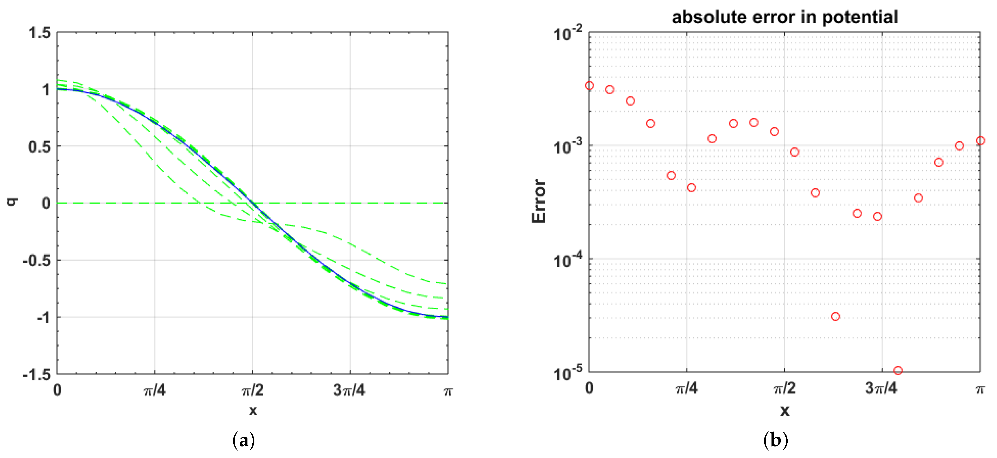
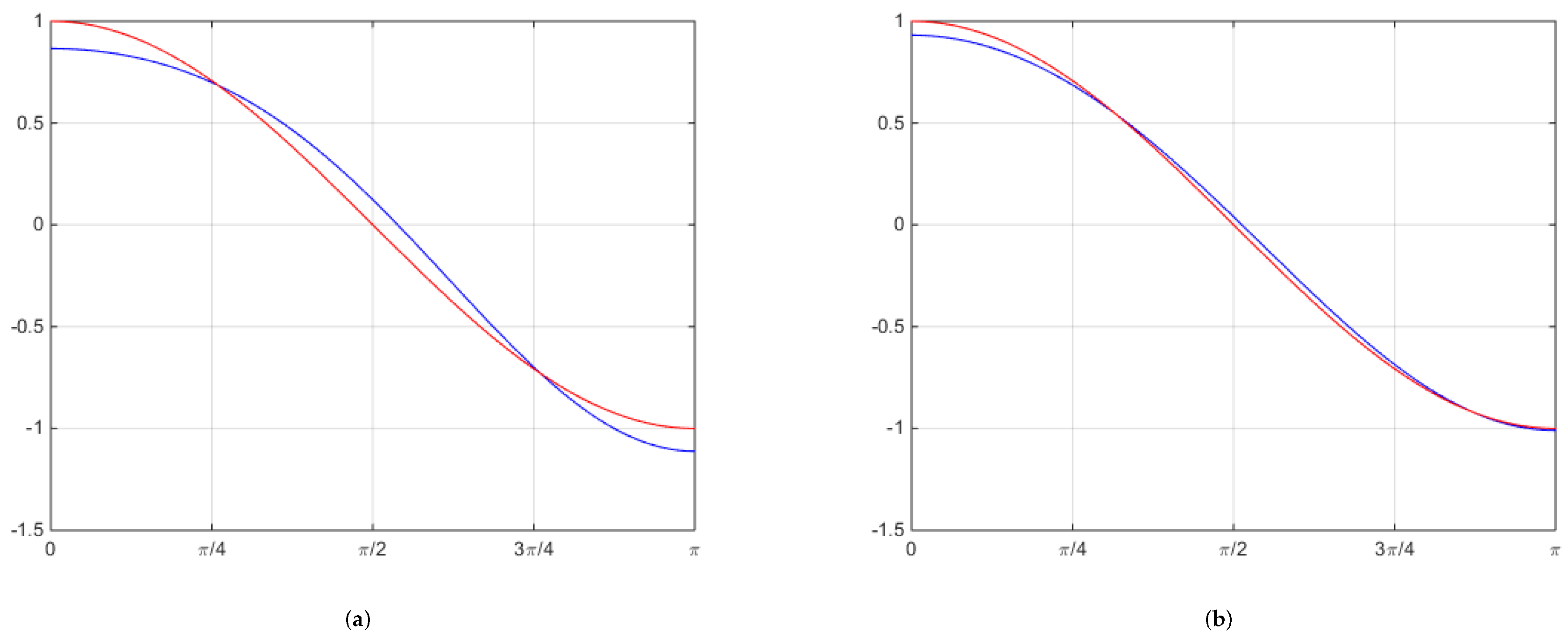
(Inverse SLP with a different domain). This example extends Barcilon’s algorithm in [36] by changing the domain $[0,1]$ to $[0,\pi ]$:

$$\begin{array}{cc}\hfill u^{″}+(\lambda -cos\left(x\right))u& =0,x\in (0,\pi )\hfill \end{array}$$

Here, $p\left(x\right)$ is symmetric and normalized. In the inverse Algorithm 1 of [39], $w_n^{\left(0\right)}\left(x\right)$ and ${\omega }_n^{\left(0\right)}\left(x\right)$ need to be changed into ${\left\{w_n^{\left(0\right)}\right\}}_1^{\infty }={\left\{cos\left(nx\right)-cos\left(n\pi \right)\right\}}_1^{\infty }$, ${\left\{{\omega }_n^{\left(0\right)}\right\}}_1^{\infty }={\{sin\left(nx\right)\}}_1^{\infty }$ which are the basic solutions in the new domain. The truncated eigenvalue sequences at $N=6$, for Dirichlet boundary conditions (DDBCs) and Dirichlet– Neumann boundary conditions (DNBCs) are calculated using the Magnus method (with $m=20$, $n=20$, $L=15$) and $M=10$ inverse algorithm steps are used.

Figure 1 shows the reconstructed and exact potential, and the log absolute errors in the reconstructed potential, respectively. From Figure 1a, it is obvious that the potential is converging towards the exact one. The max-norm of difference between the reconstructed p and the actual p is ≈$3.35\times {10}^{-3}$ and the max-norm of difference between the reconstructed eigenvalues and the actual ones is ≈$1.62\times {10}^{-3}$.

Figure 2 shows reconstructed p starting with perturbed eigenvalues

$${\sigma }_k^{\delta }={\sigma }_k+\delta {\sigma }_k·rand(size\left({\sigma }_k\right),k=1,\dots ,2N$$

where δ is the noise level and $N=5$, $m=20$, $n=100$, $L=5$, $M=6$.

It is obvious that reconstruction is possible even in the presence of a significant noise.

Example 5

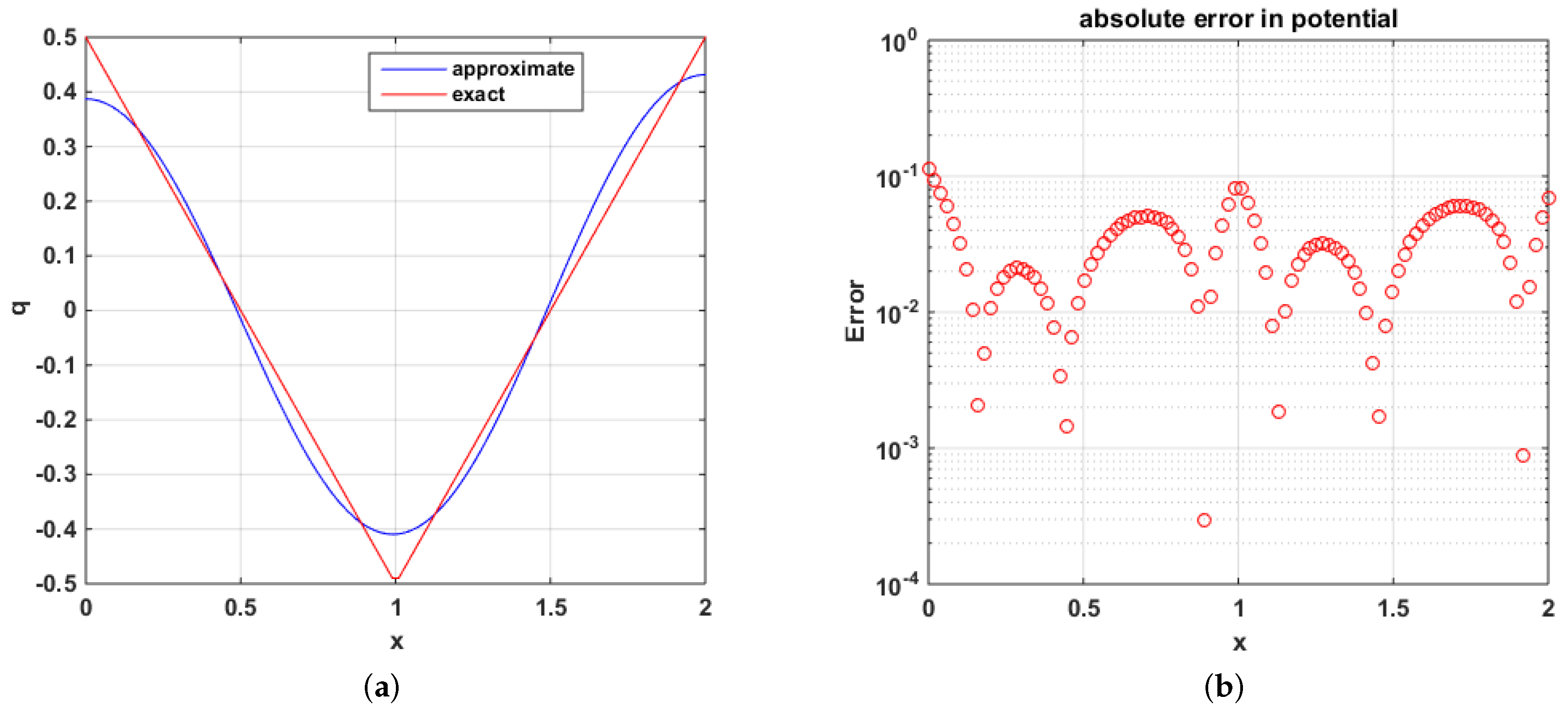
(Inverse SLP with a non-smooth potential). This example extends Barcilon’s algorithm in [36] by reconstructing a non-smooth potential:

$$\begin{array}{cc}\hfill u^{″}+(\lambda -p\left(x\right))u& =0,x\in (0,2)\hfill \end{array}$$

with $p\left(x\right)=|1-x|-0.5$: symmetric and normalized, but non-smooth. The truncated eigenvalue sequences at $N=4$, for DDBCs and DNBCs are calculated using the Magnus method (with $m=10$, $n=100$, $L=5$), and used in the reconstruction of the potential.

Figure 3 shows the reconstructed and exact potential, and the log absolute errors in the reconstructed potential, respectively, using one inverse algorithm step. From Figure 3a, it is obvious that the potential is converging towards the exact one. The max-norm of difference between the reconstructed p and the actual p is ≈$1.13\times {10}^{-1}$ and the max-norm of difference between the reconstructed eigenvalues and the actual ones is ≈$3.15\times {10}^1$. As anticipated, the error is maximum at the point of non-differentiability and at the boundaries.

Example 6

(FSLP). Consider

$$\begin{array}{cc}\hfill y^{\left(4\right)}-{\left(p_1{y}^{\prime }\right)}^{\prime }+p_{2}y& =\lambda y,0<x<\pi \hfill \end{array}$$

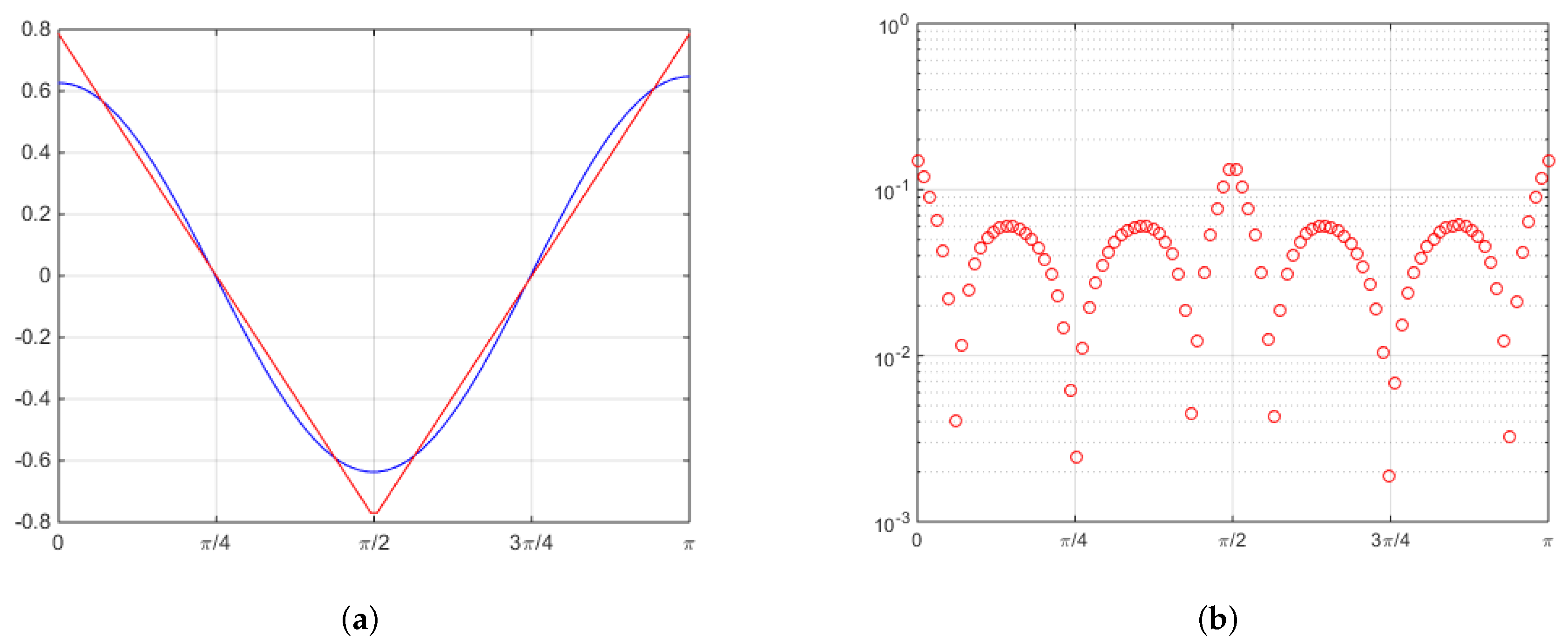
with $p_1\equiv 0$ and $p_2\left(x\right)=\pi /2-x$. Using the three spectra corresponding to the sets of BCs: $\{y\left(0\right)=y^{″}\left(0\right)=y\left(1\right)=y^{″}\left(1\right)=0\}$, $\{y\left(0\right)=y^{\prime }\left(0\right)=y\left(1\right)=y^{″}\left(1\right)=0\}$ and $\{y^{\prime }\left(0\right)=y^{″}\left(0\right)=y\left(1\right)=y^{″}\left(1\right)=0\}$ two potential functions $p_1$, $p_2$ are reconstructed starting with zero initial guesses and $N=4$, $m=20,n=100,L=5$, $M=6$ (Figure 4). The max-norm of difference between the reconstructed $p_2$ and actual $p_2$ is ≈$3.5\times {10}^{-1}$ and the max-norm of difference between the reconstructed eigenvalues and the actual ones is ≈$2.1\times {10}^{-1}$.

Example 7

(FSLP). Consider

$$\begin{array}{cc}\hfill y^{\left(4\right)}-{\left(p_1{y}^{\prime }\right)}^{\prime }+p_{2}y& =\lambda y,0<x<\pi \hfill \end{array}$$

with $p_1\left(x\right)=|x-\pi /2|-\pi /4$ and $p_2\equiv 0$. Using the three spectra corresponding to the sets of BCs: $y\left(0\right)=y^{″}\left(0\right)=y\left(1\right)=y^{″}\left(1\right)=0$, $y\left(0\right)=y^{\prime }\left(0\right)=y\left(1\right)=y^{″}\left(1\right)=0$ and $y^{\prime }\left(0\right)=y^{″}\left(0\right)=y\left(1\right)=y^{″}\left(1\right)=0$ two potential functions $p_1$, $p_2$ are reconstructed starting with zero initial guesses and $N=4$, $m=20,n=100,L=15$, $M=6$ (Figure 5). The max-norm of difference between the reconstructed $p_1$ and the actual $p_1$ is ≈$1.4\times {10}^{-1}$ and the max-norm of difference between the reconstructed eigenvalues and the actual ones is ≈$7.5\times {10}^{-1}$.

5. Discussion

In the first few examples, the Magnus method [39] is further extended to solve some direct singular SLPs on infinite domain, half-axis and for an asymmetric potential. Later, Barcilon’s algorithm is extended to solve inverse SLPs in a non–unit domain and for a non–smooth potential. The first two examples, which extend the Magnus method in [39] to infinite interval, illustrates it’s applicability to singular SLPs effectively. Furthermore, the present method does not require transforming the singular SLP to a regular one or re-scaling the eigenvalues. It effectively finds the required eigenvalues, just by truncating the interval to a finite one.

Next, the inverse SLP is solved with smooth and non-smooth potential, even in the presence of noise. It is observed that the method is successful even in the presence of significant noise, provided that the assumptions of the algorithm are satisfied.

The last few examples solve the inverse FSLP using Barcilon’s algorithm with the initial knowledge of three spectra. A simplified FSLP is solved keeping one of the unknown potential functions zero.

6. Conclusions

More than 40 years after Barcilon’s paper [36], this paper gives a concrete implementation of the inverse SLP algorithm proposed therein, to our knowledge for the first time. Furthermore, computational feasibility and applicability of this algorithm for solving inverse SLPs of higher order is verified successfully in this paper (for $n=2$ and $n=4$).

In future work, it is possible to extend the results to solve even higher order SLPs.

In conclusion, this work provides a method that can be adapted successfully for solving a direct (regular/singular) or inverse SLP of an arbitrary order with arbitrary BCs.

References

- Ambarzumian, V. Über eine frage der eigenwerttheorie. Z. Phys. A Hadron. Nucl. 1929, 53, 690–695. [Google Scholar]
- Tikhonov, A. On the uniqueness of the solution of the problem of electromagnetic sounding. Dokl. Akad. Nauk SSSR 1949, 69, 797–800. [Google Scholar]
- Levinson, N. The Inverse Sturm-Liouville Problem. Mat. Tidsskr. B 1949, 1949, 25–30. [Google Scholar]
- Marčenko, V. Sturm-Liouville Operators and Their Applications; Birkhauser Verlag: Basel, Switzerland, 1986. [Google Scholar]
- Levitan, B. Inverse Sturm-Liouville Problems; VNU Science Press: Utrecht, The Netherlands, 1987. [Google Scholar]
- Kravchenko, V.V. Direct and Inverse Sturm-Liouville Problems: A Method of Solution; Springer Nature: Berlin/Heidelberg, Germany, 2020. [Google Scholar]
- McLaughlin, J.R. Analytical methods for recovering coefficients in differential equations from spectral data. SIAM Rev. 1986, 28, 53–72. [Google Scholar] [CrossRef]
- Freiling, G.; Yurko, V.A. Inverse Sturm-Liouville Problems and Their Applications; NOVA Science Publishers: New York, NY, USA, 2001. [Google Scholar]
- Barcilon, V. Iterative solution of the inverse Sturm-Liouville problem. J. Math. Phys. 1974, 15, 429–436. [Google Scholar] [CrossRef]
- Sacks, P.E. An iterative method for the inverse Dirichlet problem. Inverse Probl. 1988, 4, 1055–1069. [Google Scholar] [CrossRef]
- Hald, O.H. The inverse Sturm-Liouville problem and the Rayleigh-Ritz method. Math. Comput. 1978, 32, 687–705. [Google Scholar] [CrossRef]
- Paine, J. A numerical method for the inverse Sturm-Liouville problem. SIAM J. Sci. Stat. Comput. 1984, 5, 149–156. [Google Scholar] [CrossRef]
- Rundell, W.; Sacks, P.E. Reconstruction techniques for classical inverse Sturm-Liouville problems. Math. Comput. 1992, 58, 161–183. [Google Scholar] [CrossRef]
- Lowe, B.D.; Pilant, M.; Rundell, W. The recovery of potentials from finite spectral data. SIAM J. Math. Anal. 1992, 23, 482–504. [Google Scholar] [CrossRef]
- Neher, M. Enclosing solutions of an inverse Sturm-Liouville problem with finite data. Computing 1994, 53, 379–395. [Google Scholar] [CrossRef]
- Fabiano, R.H.; Knobel, R.; Lowe, B.D. A finite-difference algorithm for an inverse Sturm-Liouville problem. IMA J. Numer. Anal. 1995, 15, 75–88. [Google Scholar] [CrossRef]
- Ghelardoni, P. Approximations of Sturm-Liouville eigenvalues using boundary value methods. Appl. Numer. Math. 1997, 23, 311–325. [Google Scholar] [CrossRef]
- Aceto, L.; Ghelardoni, P.; Magherini, C. BVMs for Sturm-Liouville eigenvalue estimates with general boundary conditions. J. Numer. Anal. Ind. Appl. Math 2009, 4, 113–127. [Google Scholar]
- Ghelardoni, P.; Magherini, C. BVMs for computing Sturm-Liouville symmetric potentials. Appl. Math. Comput. 2010, 217, 3032–3045. [Google Scholar] [CrossRef]
- Aceto, L.; Ghelardoni, P.; Magherini, C. Boundary value methods for the reconstruction of Sturm-Liouville potentials. Appl. Math. Comput. 2012, 219, 2960–2974. [Google Scholar] [CrossRef]
- Andrew, A.L. Numerov’s method for inverse Sturm-Liouville problems. Inverse Probl. 2005, 21, 223–238. [Google Scholar] [CrossRef]
- Andrew, A.L. Numerical solution of inverse Sturm-Liouville problems. ANZIAM J. 2004, 45, 326–337. [Google Scholar] [CrossRef]
- Andrew, A.L. Computing Sturm-Liouville potentials from two spectra. Inverse Probl. 2006, 22, 2069–2081. [Google Scholar] [CrossRef]
- Röhrl, N. A least-squares functional for solving inverse Sturm–Liouville problems. Inverse Probl. 2005, 21, 2009–2017. [Google Scholar] [CrossRef]
- Rafler, M.; Böckmann, C. Reconstruction method for inverse Sturm–Liouville problems with discontinuous potentials. Inverse Probl. 2007, 23, 933–946. [Google Scholar] [CrossRef]
- Efremova, L.; Freiling, G. Numerical solution of inverse spectral problems for Sturm-Liouville operators with discontinuous potentials. Open Math. 2013, 11, 2044–2051. [Google Scholar] [CrossRef]
- Ignatiev, M.; Yurko, V. Numerical Methods for Solving Inverse Sturm-Liouville Problems. Results Math. 2008, 52, 63–74. [Google Scholar] [CrossRef]
- Liu, C.S. Solving an inverse Sturm-Liouville problem by a Lie-group method. Bound. Value Probl. 2008, 2008, 749865. [Google Scholar] [CrossRef]
- Böckmann, C.; Kammanee, A. Broyden method for inverse non-symmetric Sturm-Liouville problems. BIT Numer. Math. 2011, 51, 513–528. [Google Scholar] [CrossRef]
- Böckmann, C.; Rattana, A. An inverse fourth order sturm-liouville problem. AIP Conf. Proc. 2015, 1648, 850030. [Google Scholar] [CrossRef]
- Gao, Q. Decent flow methods for inverse Sturm–Liouville problem. Appl. Math. Model. 2012, 36, 4452–4465. [Google Scholar] [CrossRef]
- Gao, Q.; Cheng, X.; Huang, Z. Modified Numerov’s method for inverse Sturm–Liouville problems. J. Comput. Appl. Math. 2013, 253, 181–199. [Google Scholar] [CrossRef]
- Drignei, M.C. A Newton-type method for solving an inverse Sturm-Liouville problem. Inverse Probl. Sci. Eng. 2014, 23, 851–883. [Google Scholar] [CrossRef]
- Kravchenko, V.V. On a method for solving the inverse Sturm-Liouville problem. J. Inverse Ill Posed Probl. 2018. [Google Scholar] [CrossRef]
- Neamaty, A.; Akbarpoor, S.; Yilmaz, E. Solving Symmetric Inverse Sturm-Liouville Problem Using Chebyshev Polynomials. Mediterr. J. Math. 2019, 16, 74. [Google Scholar] [CrossRef]
- Barcilon, V. On the solution of inverse eigenvalue problems of high orders. Geophys. J. Int. 1974, 39, 143–154. [Google Scholar] [CrossRef]
- McLaughlin, J.R. An Inverse Eigenvalue Problem of Order Four. SIAM J. Math. Anal. 1976, 7, 646–661. [Google Scholar] [CrossRef]
- McLaughlin, J.R. An Inverse Eigenvalue Problem of Order Four—An Infinite Case. SIAM J. Math. Anal. 1978, 9, 395–413. [Google Scholar] [CrossRef]
- Perera, U.; Böckmann, C. Solutions of Direct and Inverse Even-Order Sturm-Liouville Problems Using Magnus Expansion. Mathematics 2019, 7, 544. [Google Scholar] [CrossRef]
- Barcilon, V. On the uniqueness of inverse eigenvalue problems. Geophys. J. R. Astron. Soc. 1974, 38, 287–298. [Google Scholar] [CrossRef]
- Mathematica; Wolfram Research, Inc.: Champaign, IL, USA, 2016.
- Matlab; The MathWorks, Inc.: Natick, MA, USA, 2014.
- Taşeli, H. Accurate numerical bounds for the spectral points of singular Sturm–Liouville problems over −∞ < x < ∞. J. Comput. Appl. Math. 2000, 115, 535–546. [Google Scholar] [CrossRef]
- Marletta, M.; Pryce, J.D. Automatic solution of Sturm-Liouville problems using the Pruess method. J. Comput. Appl. Math. 1992, 39, 57–78. [Google Scholar] [CrossRef]