A Sustainable Inventory Model with Imperfect Products, Deterioration, and Controllable Emissions

Abstract

Maintaining product quality and environmental performance are emerging concerns in modern competitive and transparent businesses. Many retailers separate perfect products from imperfect ones to ensure product quality and endeavor to achieve carbon dioxide (CO₂) reduction through green technology investments and sustainable inventory planning. Product deterioration often badly hampers the retailing business; hence, suitable preservation technologies are used. In this study, we examined the optimization model of the selling price, investment, and replenishment planning to maximize the total profit. The proposed model considered the effect of a greater deterioration rate and discount price of imperfect products. Due to the high uncertainty in demand, a realistic holding cost was deliberated with a variable and constant part. Every time the retailer transports purchased items, greenhouse gases (GHGs), including CO₂, are produced. Government regulations on CO₂ minimization and customer awareness for greener products stimulate retailers to invest in energy-efficient green technology. This study simultaneously showed a harmonious relationship among the attributes of preservation technology, green technology investment, and discounts on defective items. Theoretical derivations were performed with numerical analysis.

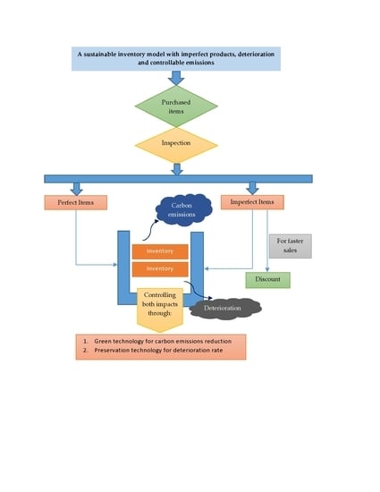
1. Introduction

The emerging intensity of the present world’s economy continually compels adjusting the economy’s configurations, which hints at massive pressure on the energy demand. Altogether, the gradually increased concern on environmental issues (e.g., greenhouse gases and waste disposal) and their consequences have become more popular in industries. In November 2007, the fourth valuation report on the environment published by the Intergovernmental Panel on Climate Change (IPCC) scrupulously indicated that greenhouse gases (including carbon dioxide/CO₂) are the main factors affecting the climate [1].

Respecting the public interest in climate change, a pact was signed by the developed countries, which was later named the Kyoto Protocol, to provide extra protection to the environment and to avoid inevitable catastrophic circumstances. The protocol is also recommended for developing countries to increase the energy-efficient tools in the production process to curb emissions. One of the major concerns of our study was that some developing countries have numerous industries (e.g., ready-made garment industries and auto rice mills) and emit CO₂ to the environment but have no policy to curb their emissions. For this type of country, a green technology investment may be suitable and energy cost-efficient. Studies showed that green technology can efficiently curb emissions in the production system as well as from the transportation system [2,3,4] in a sustainable inventory system.

Sustainable inventory management reduces the environmental effects, e.g., CO₂ emissions, of supply chain inventory [5,6]. It considers the emissions due to ordering, transporting, storing, and other material handling operations, together with the effect of the supply chain and product characteristics. Our study focused on how to curb emissions and the deterioration rate of the products. Advanced technologies, such as energy-efficient transportation technology and preservation technology, are available. Particularly, the emission reduction from energy-efficient technology may stimulate higher customer demand [2,7]. The optimum investment decision is also important because management must secure the profit margins.

These decisions can be affected by numerous attributes related to inventory management. Deterioration is one. Deterioration of products includes decay, obsolesces, evaporation, and a decrease in quality during the storage time in the warehouse. Preservation technology has been used in many industries, such as agricultural and food industries, to extend the product lifecycle and, hence, affect the total profit [8,9]. Mishra et al. [4] suggested retailer investments in green and preservation technologies to control emissions and the deterioration rate. However, in that paper, the quality inspection of the product, which is an important and realistic attribute in maintaining the retailer’s inventory, was ignored.

Considering the proposals of Gao et al. [2] and Lou et al. [7], our study extends the suggested model by incorporating the positive effect of emission reduction on customer demand. Selling price is an important attribute in the retailing business to catch the customer’s attention. In general, the higher the price of a product, the less the demand for that product. However, the retailer can optimize the selling price to balance the effect of expenses and the negative impact of price increase on customer demand. Bearing the importance of selling price, in this study, we considered the demand patterns. Our study sought to determine the optimum replenishment cycle, green technology investment, and selling price when a company attempts to maximize the profit while having concern for environmental responsibility.

The proposed model also considers the common industrial situation in which imperfect quality products occur. The defective products have a greater rate of deterioration than the perfect products [10,11]. Hence, the retailer will separate the defective products through quality inspection. Kazemi et al. [12] and Daryanto et al. [13] incorporated inspection and product separation on a sustainable inventory problem. However, the studies did not incorporate technology investment and assumed a constant demand pattern. Our study considered the joint effects of price and carbon reduction on customer demand similar to Lou et al. [7]; however, we also proposed different demand patterns between the perfect and the imperfect quality products due to a discount price being charged for the imperfect products. The proposed study also considered the holding period of the defective products. Due to uncertainty in demand, a realistic holding cost was deliberated with a variable and constant part for both the perfect and the imperfect quality products. The major contributions of this proposed model are the following.

(1)

This study aids retail managers to make optimum decisions on replenishment, selling price, and technology investment to maximize the total profit when a carbon emission tax is charged, deterioration and defective products affect the inventory level, and demand is sensitive to price and emission reductions.

(2)

We propose a model that separates the inventory of the perfect and imperfect quality products and allows a discount strategy for the imperfect items, which helps the retailer to run the business smoothly without any interruptions in the profit margin.

(3)

We studied a synergy on the reduction in product deterioration and carbon emissions for both the perfect and imperfect quality products.

This introduction section is followed by a literature review. Then, the model formulation and theoretical derivation are elaborated in Section 3. In Section 4, we illustrate the cases with examples and sensitivity analysis to obtain managerial insights. Finally, in Section 5, we conclude our findings and present potential future extensions.

2. Literature Review

This section provides a review of the related inventory model and sustainable inventory models as the foundation of our study.

2.1. Inventory Model with Defective and Deteriorating Products

Due to faulty production processes and improper handling, defective products can be produced [14,15]. In every lot of products, there are some imperfect quality items. The inspection process provides a solution by separating the products and ensuring that only the perfect products will reach the customers. Some models assumed that the retailers return the defective products to the supplier [16,17] or sell them instantaneously at a discounted price [18,19,20]. These assumptions neglect the holding cost of the defective products. In many situations, the retailer cannot sell the defective products instantaneously; hence, a holding cost is applied for the defective products [21]. Lin [22] relaxed the model by allowing the retailer to hold the defective products until several deliveries, while Wahab and Jaber [23] differentiated the holding costs charged for different product conditions. Considering a similar quality problem, our study followed the assumptions from Teng and Hsu [21], Lin [22], Wahab and Jaber [23], and Alamri et al. [24], which considered the holding period of the defective products. Our study considers the fixed and variable holding cost as an effect of time, similar to Shaikh et al. [25]. Other research also identified the imperfect quality problems in deteriorating item inventory models [26,27,28]. These studies assumed a known distribution of defective products in each received lot. Hence, a screening process with a known rate is performed to separate the defective products, which will then be sold.

Deterioration is a common attribute of products that affect the retailer’s inventory. It decreases the quality as well as the quantity of the products. For instance, fruits, vegetables, fish, etc. are examples of deteriorating products. Some items, such as vegetables, have a temporary fresh life and degrade shortly after the pluck uptime. This is known as non-instantaneous deterioration [29,30,31]. For highly deteriorating items, preservation technology can play a significant role in preserving the products. For example, ice cream is a highly deteriorating item and always seeks proper preservation. Thus, a fridge can provide the facility to preserve the ice cream. In some cases, vacuum machines are also used as a preservation tool in the retailing business.

However, both these instruments (fridge and vacuum machine) require a considerable amount of expenses to run their functions smoothly and to provide protection for the deteriorating items [32,33,34]. Hence, there is a question of how much capital can be invested in preservation technology to effectively prevent product deterioration. Similar to several previous studies, our study answered the question by optimizing the preservation of technology investment. The proposed model combined the imperfect products, investment in green technology, and its effect on customer demand.

The inventory model for deteriorating items is also affected by different demand patterns [35], such as stock level [4], selling price [36,37], and time, as the deterioration rate may increase with time [27,38,39,40]. Some items may have a random demand [41]. Recently, Saren et al. [42] studied the application of the price-discount policy for deteriorating products to attract more customers, while Mashud et al. [30] investigated a synergy between the selling price and promotion effort. Over the years, pricing strategies have caught the attention of business owners. A business runs smoothly based on important decisions, including: (1) What is the optimum selling price to sell the products in a minimum period? (2) How many customers are attracted to a price discount? Considering these questions and the presence of imperfect products, our study assumed a demand pattern based on the selling price and a discount for imperfect items. The demand was also affected by customer preferences on the retailer’s performance in lowering the emissions.

Our study also considered the general practice in the agricultural industry to control the deterioration rate by separating defective and decaying products. These kinds of products have a greater deterioration rate than perfect ones [10,11]. This affects the deterioration rate of other products. Considering this loss, Hasan et al. [43] suggested product separation after the deterioration started. For similar reasons, Khakzad and Gholamian [44] proposed multiple inspections and separations, assuming that the deterioration rate depends on the inspection frequency, which can be optimized.

2.2. Sustainable Inventory Model

Sustainable inventory management studies the environmental effects, e.g., CO₂ emissions and solid waste, to develop an environmentally responsible inventory model [45]. Studies may consider many factors, including carbon emission regulations, such as carbon tax [46,47]. Considering the presence of defective products, Sarkar et al. [5] allowed the rework of defective products. Daryanto et al. [48] studied the effect of different inspection schemes to maintain carbon emissions under carbon tax regulations. Recently, Daryanto et al. [13] developed a sustainable inventory model that separated the imperfect products and charged different holding costs. Inspired by this assumption, our study considered the same treatment while seeking to reduce emission levels through the use of green technology.

Recent studies on sustainable inventory models proposed the application of green technology to reduce emission levels [2,7]. Renewable energy and efficient energy consumption technology can be applied to reduce emissions from production, transportation, lighting, and other supporting facilities. Yang et al. [49] studied the optimal green investment in dual-channel marketing with an e-commerce platform. Investments in green technology can increase customer demand [2,7] because consumers are increasingly concerned about the environment. Taleizadeh et al. [50] studied a green supply chain with different coordination contracts when the demand was affected by the rate of carbon emission reduction. Our study also examined the optimal investment in green technology considering the effect on customer demand. Our study also extended the model from Mishra et al. [4,51], which combined the investment in green technology and preservation technology for deteriorating items. Mishra et al. [4] worked with non-instantaneous deterioration and optimized the selling price and investments. The study proved the benefit of investments to control the deterioration rate, emission rate, and order cost. Recently, Mishra et al. [51] extended the study by allowing shortages and backorder and working under the carbon tax and cap regulations.

3. Mathematical Model Formulation

This section presents the problem description, model development, and some theories derived from the total profit model. First, we list the complete notation as follows:

Notations	Description
Parameters
g	Constant part of the demand function for perfect items
g1	Constant part of the demand function for imperfect items
h	Index of price elasticity
AOC	Ordering cost per cycle
j	Coefficient of customer’s choice for low carbon
λ	Percentage of emission reduction per unit product
prc	Purchase cost per unit
h1	Unit holding cost per unit time of the perfect items
h2	Unit holding cost per unit time of the imperfect items
m	Constant part of the holding cost
n	Time-varying coefficient of the holding cost
cscr	Screening cost per unit
r	Discount rate on imperfect items
ϕ1	Deterioration rate of the perfect items
ϕ2	Deterioration rate of the imperfect items
q	Sensitive parameter of preservation technology
γ	Per unit invested amount in preservation technology
σ	Percentage of imperfect items
u	Fixed cost of transportation per trip
v	Variable cost per unit transported per distance traveled
dst	Distance traveled
nt	Number of trips
wp	Product weight
tcp	Truck capacity
Fct	Fixed cost per truck per trip
ng	No. of gallons per truck per distance traveled
e	Greenhouse gas (GHG) emissions per gallon of diesel truck fuel
Tc	Carbon emission tax per ton of GHG emissions
cfh	Fixed carbon emissions of holding inventory
cvh	Variable carbon emission factor per holding cost
π	Maximum portion of carbon emissions that can be reduced by utilizing green technology
Y	Efficiency of greener technology
Decision variables
sp	Selling price per unit
L	Replenishment cycle
G	Green investment cost in carbon reduction per cycle
Other variables
D	Demand rate for perfect items (units/year)
D1	Demand rate for imperfect items (units/year)
S	Order quantity/maximum stock per cycle
I1(t)	Level of inventory for the perfect items at time t
I2(t)	Level of inventory for the imperfect items at time t

3.1. Problem Description

In every cycle, a retailer purchases S unit of product from a supplier and transports them to their warehouse by truck. In this process, carbon dioxide is emitted. The lead time between the order submission and the receipt is considered negligible. A percentage of the product is damaged during the loading, unloading, and traveling process. Hence, upon unloading the products, the retailer runs inspection processes where the perfect and imperfect items are identified and separated. A σ portion of total products is found imperfect, while the remaining (1 − σ) portion is perfect. The retailer charges discounted prices for imperfect items to influence customer demand. Figure 1 illustrates the inventory level.

The retailer runs the business in an environmentally conscious manner, similar to Lou et al. [7]. Hence, the demand pattern for the perfect items is $D(s_p,\lambda )=g-h{s}_p+j\lambda$ and $D_1(s_p,\lambda )=g_1-h\left[\left(1-r\right)s_p\right]+j\lambda ,$ for the imperfect items, where g, g₁, h > 0. Here, j is the coefficient of customer choice for low carbon, and the demand is easily influenced by j when λ is high (motivated by Gao et al. [2] and Lou et al. [7]).

The retailer maintains product deterioration. For this reason, they use preservation technology to hold the products for a longer time. The deterioration rate of imperfect items is considered higher than for perfect items as imperfect items deteriorate faster than the perfect items. Using preservation technology, the rate of deterioration is reduced by using $p\left(\gamma \right)=e^{-q\gamma },$ which satisfies $\frac{\partial p\left(\gamma \right)}{\partial \gamma }<0 , \frac{{\partial }^{2}p\left(\gamma \right)}{\partial {\gamma }^2}>0$. Here, $\gamma$ denotes the investment and q is the sensitive parameter of investment, as in He and Huang [8] and Mishra et al. [9].

Considering the effect of carbon reduction, preservation technology, and price setting on customer demand, the retailer specifies the optimum selling price, investment in green technology, and the inventory cycle time.

3.2. Mathematical Forms of the Proposed Model

There are two types of products considered for the model. Thus, the level of inventory for both types is different from each other according to their characteristics. The differential equation that presents the inventory for the perfect items is:

$$\frac{d{I}_1\left(t\right)}{dt}+{\varphi }_{1}p\left(\gamma \right)I_1\left(t\right)=-D, 0\le t\le L$$

(1)

with $I_1\left(0\right)=\left(1-\sigma \right)S \mathrm{and} I_1\left(L\right)=0$.

The differential equation that presents the inventory for the imperfect items differs in terms of product consumption. Thus, demand is considered different. The equation is:

$$\frac{d{I}_2\left(t\right)}{dt}+{\varphi }_{2}p\left(\gamma \right)I_2\left(t\right)=-D_1, 0\le t\le L_1$$

(2)

$\mathrm{with} I_2\left(0\right)=\sigma S \mathrm{and} I_2\left(L_1\right)=0$.

Solving the above equations based on the given boundary conditions, we obtain the level of inventory for the perfect items

$$I_1\left(t\right)=\frac{D}{{\varphi }_{1}p\left(\gamma \right)}\left[e^{{\varphi }_{1}p\left(\gamma \right)\left(L-t\right)}-1\right]$$

(3)

and the level of inventory for the imperfect items

$$I_2\left(t\right)=\frac{D_1}{{\varphi }_{2}p\left(\gamma \right)}\left[e^{{\varphi }_{2}p\left(\gamma \right)\left(L_1-t\right)}-1\right].$$

(4)

Now, using the boundary condition for the perfect item $I_1\left(0\right)=\left(1-\sigma \right)S$ in Equation (3), we have the initial stock for the retailer

$$S=\frac{D}{\left(1-\sigma \right){\varphi }_{1}p\left(\gamma \right)}\left[e^{{\varphi }_{1}p\left(\gamma \right)L}-1\right].$$

(5)

Because the demand for the imperfect items, in most cases, is lower than the demand for the perfect items and the rate of deterioration for imperfect items is slightly faster than for perfect items, the retailer decides to sell them at a discount price with a rate $r\%$ that adds sales revenue. Thus, the entire sales revenue becomes:

$$\begin{gathered} \mathrm{SR}=s_{p}D{\displaystyle \underset{0}{\overset{L}{\int }}dt+}\left(1-r\right)s_p{D}_1{\displaystyle \underset{0}{\overset{L_1}{\int }}dt} \\ =s_{p}DL+\left(1-r\right)s_p{D}_1{L}_1. \end{gathered}$$

(6)

The ordering cost per cycle is

$$\mathrm{OC}=\frac{A_{oc}}{L}.$$

(7)

The purchasing cost per cycle is

$$\begin{gathered} \mathrm{PC}=\frac{p_{rc}S}{L} \\ =\frac{p_{rc}D}{\left(1-\sigma \right){\varphi }_{1}p\left(\gamma \right)L}\left[e^{{\varphi }_{1}p\left(\gamma \right)L}-1\right]. \end{gathered}$$

(8)

Now, a cost-saving screening process is run by the retailer. For the whole screening process, the screening cost per cycle is

$$\begin{gathered} \mathrm{SC}=\frac{c_{scr}S}{L} \\ =\frac{c_{scr}D}{\left(1-\sigma \right){\varphi }_{1}p\left(\gamma \right)L}\left[e^{{\varphi }_{1}p\left(\gamma \right)L}-1\right]. \end{gathered}$$

(9)

Since there are two types of products, the retailer holds them in two different places. Thus, the holding cost is implemented in two different ways for the two different types of products. The holding cost for the perfect items per cycle is

$$\begin{gathered} {\mathrm{HC}}_1=\frac{h_1}{L}{\displaystyle \underset{0}{\overset{L}{\int }}\left(m+nt\right)I_1\left(t\right)dt} \\ =\frac{h_{1}D}{{\varphi }_{1}p\left(\gamma \right)L}\left[\left\{\frac{m}{{\varphi }_{1}p\left(\gamma \right)}+\frac{n}{{\left({\varphi }_{1}p\left(\gamma \right)\right)}^2}\right\}\left[e^{{\varphi }_{1}p\left(\gamma \right)L}-1\right]-\frac{nL}{{\varphi }_{1}p\left(\gamma \right)}-mL-\frac{n{L}^2}{2}\right] . \end{gathered}$$

(10)

The holding cost for the imperfect items per cycle is

$$\begin{gathered} {\mathrm{HC}}_2=\frac{h_2}{L}{\displaystyle \underset{0}{\overset{L_1}{\int }}\left(m+nt\right)I_2\left(t\right)dt} \\ \hspace{1em}\hspace{1em}\hspace{1em}=\frac{h_2{D}_1}{{\varphi }_{2}p\left(\gamma \right)L}\left[\left\{\frac{m}{{\varphi }_{2}p\left(\gamma \right)}+\frac{n}{{\left({\varphi }_{2}p\left(\gamma \right)\right)}^2}\right\}\left[e^{{\varphi }_{2}p\left(\gamma \right)L_1}-1\right]-\frac{n{L}_1}{{\varphi }_{2}p\left(\gamma \right)}-m{L}_1-\frac{n{L}_1{}^2}{2}\right]. \end{gathered}$$

(11)

As both types of products must be held by the retailer, the aggregate holding cost per cycle is

$$\mathrm{HC}={\mathrm{HC}}_1+H{C}_2.$$

(12)

Another important issue that needs to be controlled in a very sophisticated way is product transportation. Transportation has a direct impact on the environment as it consumes fuel and emits carbon dioxide. Considering all these issues with some other features (e.g., the distance traveled, number of trips, carbon tax, product weight, and truck capacity), the transportation cost per cycle is

$$\mathrm{TRNC}=\left(2u+2v{d}_{st}{w}_{p}S\right)\frac{n_{t}S{F}_{ct}}{t_{cp}L} .$$

(13)

The preservation cost per cycle is addressed as follows:

$$\mathrm{PRC}=\frac{1}{L}\left(\gamma L\right).$$

(14)

The carbon emission cost per cycle is

$$\mathrm{CEC}=\frac{T_c}{L}\left[\left(c_{fh}+c_{vh}{w}_{p}S\right)+\frac{2d_{st}{n}_{g}e}{t_{cp}}\right].$$

(15)

Finally, we can derive

$$\begin{gathered} \alpha =\mathrm{SR}-\mathrm{OC}-\mathrm{PC}-\mathrm{SC}-\mathrm{HC}-\mathrm{TRNC}-\mathrm{PRC}-\mathrm{CEC} \\ =\frac{1}{L}\left[\begin{array}{l}{s}_{p}DL+\left(1-r\right)s_p{D}_1{L}_1-A_{oc}-\frac{p_{rc}D}{\left(1-\sigma \right){\varphi }_{1}p\left(\gamma \right)}\left[e^{{\varphi }_{1}p\left(\gamma \right)L}-1\right]-\frac{c_{scr}D}{\left(1-\sigma \right){\varphi }_{1}p\left(\gamma \right)}\left[e^{{\varphi }_{1}p\left(\gamma \right)L}-1\right]\\ -\frac{h_{1}D}{{\varphi }_{1}p\left(\gamma \right)}\left[\left\{\frac{m}{{\varphi }_{1}p\left(\gamma \right)}+\frac{n}{{\left({\varphi }_{1}p\left(\gamma \right)\right)}^2}\right\}\left[e^{{\varphi }_{1}p\left(\gamma \right)L}-1\right]-\frac{nL}{{\varphi }_{1}p\left(\gamma \right)}-mL-\frac{n{L}^2}{2}\right] \\ -\frac{h_2{D}_1}{{\varphi }_{2}p\left(\gamma \right)}\left[\left\{\frac{m}{{\varphi }_{2}p\left(\gamma \right)}+\frac{n}{{\left({\varphi }_{2}p\left(\gamma \right)\right)}^2}\right\}\left[e^{{\varphi }_{2}p\left(\gamma \right)L_1}-1\right]-\frac{n{L}_1}{{\varphi }_{2}p\left(\gamma \right)}-m{L}_1-\frac{n{L}_1{}^2}{2}\right]\\ -\left(2u+2v{d}_{st}{w}_{p}S\right)\frac{n_{t}S{F}_{ct}}{t_{cp}}-\gamma L-T_c\left[\left(c_{fh}+c_{vh}{w}_{p}S\right)+\frac{2d_{st}{n}_{g}e}{t_{cp}}\right]\end{array}\right]. \end{gathered}$$

(16)

3.3. Investment in Carbon Emission Reduction

By investing a particular amount G, the retailer reduces the per-unit carbon emissions by λ percentage, as previously implemented by Lou et al. [7] and Datta et al. [52]. The percentage of reduction can be written as λ = π(1 − e^−YG). The λ becomes zero when G = 0. When G → ∞, λ tends to π, where π denotes the maximum portion of carbon emissions from utilizing green technology and Y is the efficiency level. Then, the green investment cost per cycle is

$$GIC=\frac{1}{L}\left(GL\right).$$

(17)

With this investment, the retailer’s profit becomes

$$\alpha =\frac{1}{L}\left[\begin{array}{l}{s}_{p}DL+\left(1-r\right)s_p{D}_1{L}_1-A_{oc}-\frac{p_{rc}D}{\left(1-\sigma \right){\varphi }_{1}p\left(\gamma \right)}\left[e^{{\varphi }_{1}p\left(\gamma \right)L}-1\right]-\frac{c_{scr}D}{\left(1-\sigma \right){\varphi }_{1}p\left(\gamma \right)}\left[e^{{\varphi }_{1}p\left(\gamma \right)L}-1\right]\\ -\frac{h_{1}D}{{\varphi }_{1}p\left(\gamma \right)}\left[\left\{\frac{m}{{\varphi }_{1}p\left(\gamma \right)}+\frac{n}{{\left({\varphi }_{1}p\left(\gamma \right)\right)}^2}\right\}\left[e^{{\varphi }_{1}p\left(\gamma \right)L}-1\right]-\frac{nL}{{\varphi }_{1}p\left(\gamma \right)}-mL-\frac{n{L}^2}{2}\right] \\ -\frac{h_2{D}_1}{{\varphi }_{2}p\left(\gamma \right)}\left[\left\{\frac{m}{{\varphi }_{2}p\left(\gamma \right)}+\frac{n}{{\left({\varphi }_{2}p\left(\gamma \right)\right)}^2}\right\}\left[e^{{\varphi }_{2}p\left(\gamma \right)L_1}-1\right]-\frac{n{L}_1}{{\varphi }_{2}p\left(\gamma \right)}-m{L}_1-\frac{n{L}_1{}^2}{2}\right]\\ -\left(2u+2v{d}_{st}{w}_{p}S\right)\frac{n_{t}S{F}_{ct}}{t_{cp}}-\gamma L-T_c\left[\left(c_{fh}+c_{vh}{w}_{p}S\right)+\frac{2d_{st}{n}_{g}e}{t_{cp}}\right]\left(1-\lambda \right)-GL\end{array}\right].$$

(18)

3.4. Theoretical Derivation

Proposition 1. 

The retailer’s profit function α(s_p, G, L) presented in Equation (18) demonstrates the concavity in terms of replenishment cycle L when the selling price s_p and investment in green technology G are deliberated as constants and the optimal L* is as characterized by the following equation:

$$\begin{array}{l}L=L^{*}=\sqrt[3]{\left(\frac{-{\rho }_2{}^3}{27{\rho }_1{}^3}+\frac{{\rho }_2{\rho }_3}{6{\rho }_1{}^2}-\frac{{\rho }_4}{2{\rho }_1}\right)+\sqrt{{\left(\frac{-{\rho }_2{}^3}{27{\rho }_1{}^3}+\frac{{\rho }_2{\rho }_3}{6{\rho }_1{}^2}-\frac{{\rho }_4}{2{\rho }_1}\right)}^2+{\left(\frac{{\rho }_3}{3{\rho }_1}-\frac{{\rho }_2{}^2}{9{\rho }_1{}^2}\right)}^3}}\\ +\sqrt[3]{\left(\frac{-{\rho }_2{}^3}{27{\rho }_1{}^3}+\frac{{\rho }_2{\rho }_3}{6{\rho }_1{}^2}-\frac{{\rho }_4}{2{\rho }_1}\right)-\sqrt{{\left(\frac{-{\rho }_2{}^3}{27{\rho }_1{}^3}+\frac{{\rho }_2{\rho }_3}{6{\rho }_1{}^2}-\frac{{\rho }_4}{2{\rho }_1}\right)}^2+{\left(\frac{{\rho }_3}{3{\rho }_1}-\frac{{\rho }_2{}^2}{9{\rho }_1{}^2}\right)}^3}}-\frac{{\rho }_2}{3{\rho }_1}\end{array}$$

Proof. 

To prove the concavity, one needs to differentiate Equation (18) with respect to L as follows:

$$\frac{\partial \alpha }{\partial L}=\frac{1}{L}\left[\begin{array}{l}\left\{\frac{1}{L}\left[e^{{\varphi }_{1}p\left(\gamma \right)L}-1\right]-{\varphi }_{1}p\left(\gamma \right)e^{{\varphi }_{1}p\left(\gamma \right)L}\right\}{\mathsf{\Omega }}_1+\frac{1}{L}{\mathsf{\Omega }}_2-\frac{n{h}_{1}DL}{2{\varphi }_{1}p\left(\gamma \right)}\\ +\left\{2{\varphi }_{1}p\left(\gamma \right)e^{{\varphi }_{1}p\left(\gamma \right)L}\left[e^{{\varphi }_{1}p\left(\gamma \right)L}-1\right]-\frac{1}{L}\left[e^{{\varphi }_{1}p\left(\gamma \right)L}-1\right]\right\}{\mathsf{\Omega }}_3\end{array}\right].$$

(19)

Now, equating it to zero, one has

$$\begin{array}{l}L=\sqrt[3]{\left(\frac{-{\rho }_2{}^3}{27{\rho }_1{}^3}+\frac{{\rho }_2{\rho }_3}{6{\rho }_1{}^2}-\frac{{\rho }_4}{2{\rho }_1}\right)+\sqrt{{\left(\frac{-{\rho }_2{}^3}{27{\rho }_1{}^3}+\frac{{\rho }_2{\rho }_3}{6{\rho }_1{}^2}-\frac{{\rho }_4}{2{\rho }_1}\right)}^2+{\left(\frac{{\rho }_3}{3{\rho }_1}-\frac{{\rho }_2{}^2}{9{\rho }_1{}^2}\right)}^3}}\\ +\sqrt[3]{\left(\frac{-{\rho }_2{}^3}{27{\rho }_1{}^3}+\frac{{\rho }_2{\rho }_3}{6{\rho }_1{}^2}-\frac{{\rho }_4}{2{\rho }_1}\right)-\sqrt{{\left(\frac{-{\rho }_2{}^3}{27{\rho }_1{}^3}+\frac{{\rho }_2{\rho }_3}{6{\rho }_1{}^2}-\frac{{\rho }_4}{2{\rho }_1}\right)}^2+{\left(\frac{{\rho }_3}{3{\rho }_1}-\frac{{\rho }_2{}^2}{9{\rho }_1{}^2}\right)}^3}}-\frac{{\rho }_2}{3{\rho }_1}=L^{*}\end{array}$$

(20)

where

$$\begin{array}{l}{\mathsf{\Omega }}_1=\frac{D}{\left(1-\sigma \right){\varphi }_{1}p\left(\gamma \right)}\left\{p_{rc}+c_{scr}+\left(1-\lambda \right)T_c{c}_{vh}{w}_p+\frac{2u{n}_t{F}_{ct}}{t_{cp}}\right\}+\frac{h_{1}D}{{\varphi }_{1}p\left(\gamma \right)}\left\{\frac{m}{{\varphi }_{1}p\left(\gamma \right)}+\frac{n}{{\left({\varphi }_{1}p\left(\gamma \right)\right)}^2}\right\},\\ \begin{array}{l}{\mathsf{\Omega }}_2=\left(1-r\right)s_p{D}_1{L}_1-A_{oc}-\frac{h_2{D}_1}{{\varphi }_{2}p\left(\gamma \right)}\left[\left\{\frac{m}{{\varphi }_{2}p\left(\gamma \right)}+\frac{n}{{\left({\varphi }_{2}p\left(\gamma \right)\right)}^2}\right\}\left[e^{{\varphi }_{2}p\left(\gamma \right)L_1}-1\right]-\frac{n{L}_1}{{\varphi }_{2}p\left(\gamma \right)}-m{L}_1-\frac{n{L}_1{}^2}{2}\right]\\ -T_c\left(1-\lambda \right)\left(c_{fh}+\frac{2d_{st}{n}_{g}e}{t_{cp}}\right),\end{array}\\ {\mathsf{\Omega }}_3=\frac{2v{d}_{st}{w}_p{n}_t{F}_{ct}{D}^2}{t_{cp}{\left(1-\sigma \right)}^2{\left({\varphi }_{1}p\left(\gamma \right)\right)}^2},{\rho }_1=2{\left\{{\varphi }_{1}p\left(\gamma \right)\right\}}^3{\mathsf{\Omega }}_3,\\ {\rho }_2=2{\left\{{\varphi }_{1}p\left(\gamma \right)\right\}}^3{\mathsf{\Omega }}_3-{\left\{{\varphi }_{1}p\left(\gamma \right)\right\}}^2{\mathsf{\Omega }}_1-\frac{n{h}_{1}D}{2{\varphi }_{1}p\left(\gamma \right)}, {\rho }_3={\varphi }_{1}p\left(\gamma \right){\mathsf{\Omega }}_3, {\rho }_4={\mathsf{\Omega }}_2.\end{array}$$

Now, differentiating Equation (19) with respect to $L$, one has

$$\frac{{\partial }^2\alpha }{\partial L^2}=-\frac{1}{L}{\mathsf{\Omega }}_1{\left\{{\varphi }_{1}p\left(\gamma \right)\right\}}^2\left[{\varphi }_{1}p\left(\gamma \right)L-1\right]+\frac{2}{L^3}{\mathsf{\Omega }}_2-4{\mathsf{\Omega }}_3{\left\{{\varphi }_{1}p\left(\gamma \right)\right\}}^3.$$

(21)

To check the feasibility $L=L^{*}$, let us substitute the value of L in (21),

$${\left[\frac{{\partial }^2\alpha }{\partial L^2}\right]}_{L=L^{*}}=-\frac{1}{L^{*}}{\mathsf{\Omega }}_1{\left\{{\varphi }_{1}p\left(\gamma \right)\right\}}^2\left[{\varphi }_{1}p\left(\gamma \right)L^{*}-1\right]+\frac{2}{L^{*}{}^3}{\mathsf{\Omega }}_2-4{\mathsf{\Omega }}_3{\left\{{\varphi }_{1}p\left(\gamma \right)\right\}}^3<0.$$

(22)

To show that the above second-order derivative is negative, it is necessary to show the nature of its terms. □

Corollary 1. 

For all fixed positive parameters, if the sum of terms $\frac{1}{L^{*}}{\mathsf{\Omega }}_1{\left\{{\varphi }_{1}p\left(\gamma \right)\right\}}^2\left[{\varphi }_{1}p\left(\gamma \right)L^{*}-1\right]$ and $4{\mathsf{\Omega }}_3{\left\{{\varphi }_{1}p\left(\gamma \right)\right\}}^3$ is greater than $\frac{2}{L^{*}{}^3}{\mathsf{\Omega }}_2$, then α(s_p, G, L) satisfies the sufficient condition for the maximum value L = L*.

Proof: 

Appendix A □

Now, employing Corollary 1, in Equation (22), one can easily conclude that

${\left[\frac{{\partial }^2\alpha }{\partial L^2}\right]}_{L=L^{*}}=-\frac{1}{L^{*}}{\mathsf{\Omega }}_1{\left\{{\varphi }_{1}p\left(\gamma \right)\right\}}^2\left[{\varphi }_{1}p\left(\gamma \right)L^{*}-1\right]+\frac{2}{L^{*}{}^3}{\mathsf{\Omega }}_2-4{\mathsf{\Omega }}_3{\left\{{\varphi }_{1}p\left(\gamma \right)\right\}}^3<0$, which completes the proof.

Other propositions are proposed concerning the profit function concavity as Propositions 2 and 3.

Proposition 2. 

The retailer’s profit function α(s_p, G, L) demonstrates the concavity of s_p and entails a unique optimum s_p* when G and L are considered as constants.

Proof: 

Similar to that of Proposition 1. □

Proposition 3. 

The retailer’s profit function α(s_p, G, L) demonstrates the concavity of G and entails a unique solution G* when s_p and L are considered as constants.

Proof: 

Similar to that of Proposition 1. □

If the replenishment cycle L is considered fixed and all other decision parameters are variables, then the concavity of the profit for the retailers is explained in Proposition 4.

Proposition 4. 

The retailer’s profit function α(s_p, G, L) demonstrates the concavity of s_p and G when L is considered as constant and is characterized by the following equations:

$$\begin{gathered} s_p{}^{*}={\Delta }_4+\lambda {\Delta }_5 \\ {G}^{*}=\frac{{\Delta }_8}{2}+\sqrt{\frac{{\Delta }_8{}^2-{\Delta }_9}{4}}. \end{gathered}$$

Proof: 

Differentiating Equation (18) with respect to s_p □

$$\frac{\partial \alpha }{\partial s_p}=\frac{1}{L}\left[\left(g-2h{s}_p+j\lambda \right)L+\left(1-r\right)\left\{g_1-2h\left(1-r\right)s_p+j\lambda \right\}+h{\Delta }_1+h\left(1-r\right){\Delta }_2-\lambda h{\Delta }_3\right].$$

(23)

Now, equating it to zero, one has

$$s_p={\Delta }_4+\lambda {\Delta }_5=s_p{}^{*},$$

(24)

where

$$\begin{array}{l}{\Delta }_1=\frac{\left[e^{{\varphi }_{1}p\left(\gamma \right)L}-1\right]}{\left(1-\sigma \right){\varphi }_{1}p\left(\gamma \right)}\left(p_{rc}+c_{scr}+c_{vh}{w}_p{T}_c+\frac{2u{n}_t{F}_{ct}}{t_{cp}}\right)+\frac{h_1}{{\varphi }_{1}p\left(\gamma \right)}\left[\begin{array}{l}\left\{\frac{m}{{\varphi }_{1}p\left(\gamma \right)}+\frac{n}{{\left({\varphi }_{1}p\left(\gamma \right)\right)}^2}\right\}\left[e^{{\varphi }_{1}p\left(\gamma \right)L}-1\right]\\ -\frac{nL}{{\varphi }_{1}p\left(\gamma \right)}-mL-\frac{n{L}^2}{2}\end{array}\right]\\ {\Delta }_2=\frac{h_2}{{\varphi }_{2}p\left(\gamma \right)}\left[\left\{\frac{m}{{\varphi }_{2}p\left(\gamma \right)}+\frac{n}{{\left({\varphi }_{2}p\left(\gamma \right)\right)}^2}\right\}\left[e^{{\varphi }_{2}p\left(\gamma \right)L_1}-1\right]-\frac{n{L}_1}{{\varphi }_{2}p\left(\gamma \right)}-m{L}_1-\frac{n{L}_1{}^2}{2}\right],\\ {\Delta }_3=\frac{c_{vh}{w}_p{T}_c}{\left(1-\sigma \right){\varphi }_{1}p\left(\gamma \right)}\left[e^{{\varphi }_{1}p\left(\gamma \right)L}-1\right], {\Delta }_4=\frac{h{\Delta }_1+h\left(1-r\right){\Delta }_2+gL+\left(1-r\right)g_1{L}_1}{2hL+2h{\left(1-r\right)}^2{L}_1},\\ {\Delta }_5=\frac{jL+\left(1-r\right)j{L}_1-h{\Delta }_3}{2hL+2h{\left(1-r\right)}^2{L}_1}.\end{array}$$

By substituting the value of s_p in the profit function (18), one has

$$\alpha =\frac{1}{L}\left[\begin{array}{l}{s}_p{}^{*}DL+\left(1-r\right)s_p{}^{*}{D}_1{L}_1-A_{oc}-\frac{\left(p_{rc}+c_{scr}\right)\left(g-h{s}_p{}^{*}+j\lambda \right)}{\left(1-\sigma \right){\varphi }_{1}p\left(\gamma \right)}\left[e^{{\varphi }_{1}p\left(\gamma \right)L}-1\right]\\ -\frac{h_1\left(g-h{s}_p{}^{*}+j\lambda \right)}{{\varphi }_{1}p\left(\gamma \right)}\left[\left\{\frac{m}{{\varphi }_{1}p\left(\gamma \right)}+\frac{n}{{\left({\varphi }_{1}p\left(\gamma \right)\right)}^2}\right\}\left[e^{{\varphi }_{1}p\left(\gamma \right)L}-1\right]-\frac{nL}{{\varphi }_{1}p\left(\gamma \right)}-mL-\frac{n{L}^2}{2}\right] \\ -\frac{h_2\left(g_1-h\left(1-r\right)s_p{}^{*}+j\lambda \right)}{{\varphi }_{2}p\left(\gamma \right)}\left[\begin{array}{l}\left\{\frac{m}{{\varphi }_{2}p\left(\gamma \right)}+\frac{n}{{\left({\varphi }_{2}p\left(\gamma \right)\right)}^2}\right\}\left[e^{{\varphi }_{2}p\left(\gamma \right)L_1}-1\right]\\ -\frac{n{L}_1}{{\varphi }_{2}p\left(\gamma \right)}-m{L}_1-\frac{n{L}_1{}^2}{2}\end{array}\right]\\ -\left(2u+2v{d}_{st}{w}_{p}S\right)\frac{n_{t}S{F}_{ct}}{t_{cp}}-\gamma L-T_c\left[\left(c_{fh}+c_{vh}{w}_{p}S\right)+\frac{2d_{st}{n}_{g}e}{t_{cp}}\right]\left(1-\lambda \right)-GL\end{array}\right].$$

(25)

Let us take the first and second derivatives of (25) with respect to G as follows:

$$\frac{\partial \alpha }{\partial G}=\frac{1}{L}\left[\pi Y{\Delta }_6{e}^{-YG}-2{\pi }^{2}Y{\Delta }_7{e}^{-YG}\left(1-e^{-YG}\right)-L\right]$$

(26)

$$\frac{{\partial }^2\alpha }{\partial G^2}=-\frac{1}{L}\left[\pi Y{\Delta }_6{e}^{-YG}-2{\pi }^2{Y}^2{\Delta }_7\left\{e^{-2YG}-e^{-YG}\left(1-e^{-YG}\right)\right\}\right].$$

(27)

Now, we take $\frac{\partial \alpha }{\partial G}=0$ and then solve for G, and one has

$$G=\frac{{\Delta }_8}{2}\pm \sqrt{\frac{{\Delta }_8{}^2-{\Delta }_9}{4}}.$$

Here, we considered the positive root

$$G=\frac{{\Delta }_8}{2}+\sqrt{\frac{{\Delta }_8{}^2-{\Delta }_9}{4}}=G^{*},$$

(28)

where

$$\begin{array}{l}\begin{array}{l}{\Delta }_6=g{\Delta }_3-j\left({\Delta }_1-{\Delta }_2+{\Delta }_3\right)-2{\Delta }_4{\Delta }_5\left\{hL+{\left(1-r\right)}^{2}h{L}_1\right\}+{\Delta }_4\left\{jL+\left(1-r\right)j{L}_1-h{\Delta }_3\right\}\\ +{\Delta }_5\left\{gL+\left(1-r\right)g_1{L}_1+h{\Delta }_1+h\left(1-r\right){\Delta }_2\right\}+T_c\left(c_{fh}+\frac{2d_{st}{n}_{g}e}{t_{cp}}\right),\end{array}\\ {\Delta }_7={\Delta }_5{}^2\left\{hL+{\left(1-r\right)}^{2}h{L}_1\right\}-{\Delta }_5\left\{jL+\left(1-r\right)j{L}_1-h{\Delta }_3\right\}, {\Delta }_8=\frac{\pi Y^2{\Delta }_6+2{\pi }^{2}Y{\Delta }_7}{2{\pi }^2{Y}^2{\Delta }_7}, \mathrm{and}\\ {\Delta }_9=\frac{2\left(\pi Y{\Delta }_6-L\right)}{{\pi }^2{Y}^2{\Delta }_7}.\end{array}$$

To check the feasibility at G = G*, let us expand Equation (27) in the Taylor series and then substitute the value of G as follows:

$${\left[\frac{{\partial }^2\alpha }{\partial G^2}\right]}_{G=G^{*}}=-\frac{1}{L}\left[\pi Y^2{\Delta }_6\left(1-Y{G}^{*}\right)+6{\pi }^2{Y}^3{\Delta }_7{G}^{*}-2{\pi }^2{Y}^2{\Delta }_7\left(1+Y^2{G}^{*}{}^2\right)\right]<0.$$

(29)

To show that the above equation provides a negative value, one needs to show that the $\left[\pi Y^2{\Delta }_6\left(1-Y{G}^{*}\right)+6{\pi }^2{Y}^3{\Delta }_7{G}^{*}-2{\pi }^2{Y}^2{\Delta }_7\left(1+Y^2{G}^{*}{}^2\right)\right]$ term is positive.

Corollary 2. 

For all fixed positive parameters, if the term $\left[\pi Y^2{\Delta }_6\left(1-Y{G}^{*}\right)+6{\pi }^2{Y}^3{\Delta }_7{G}^{*}-2{\pi }^2{Y}^2{\Delta }_7\left(1+Y^2{G}^{*}{}^2\right)\right]$ presents a positive result, then Equation (29) satisfies the conditions for the maximum profit of the retailer.

Proof: 

See Appendix B □

With the help of Corollary 2, one can easily prove that Equation (29) provides a negative result. Consequently,${\left[\frac{{\partial }^2\alpha }{\partial G^2}\right]}_{G=G^{*}}=-\frac{1}{L}\left[\pi Y^2{\Delta }_6\left(1-Y{G}^{*}\right)+6{\pi }^2{Y}^3{\Delta }_7{G}^{*}-2{\pi }^2{Y}^2{\Delta }_7\left(1+Y^2{G}^{*}{}^2\right)\right]<0$, which completes the proof.

In addition, Propositions 5 and 6 are proposed by keeping one decision variable as constant and others as variables.

Proposition 5. 

The profit function α(s_p, G, L) demonstrates the concavity of G and L when s_p is considered as constant and this entails a unique solution (G*, L*).

Proof: 

Similar to that of Proposition 4. □

Proposition 6. 

The profit function α(s_p, G, L) demonstrates the concavity of s_p and L when G is considered as constant and this entails a unique solution (s_p *, L*)

Proof: 

Similar to that of Proposition 4. □

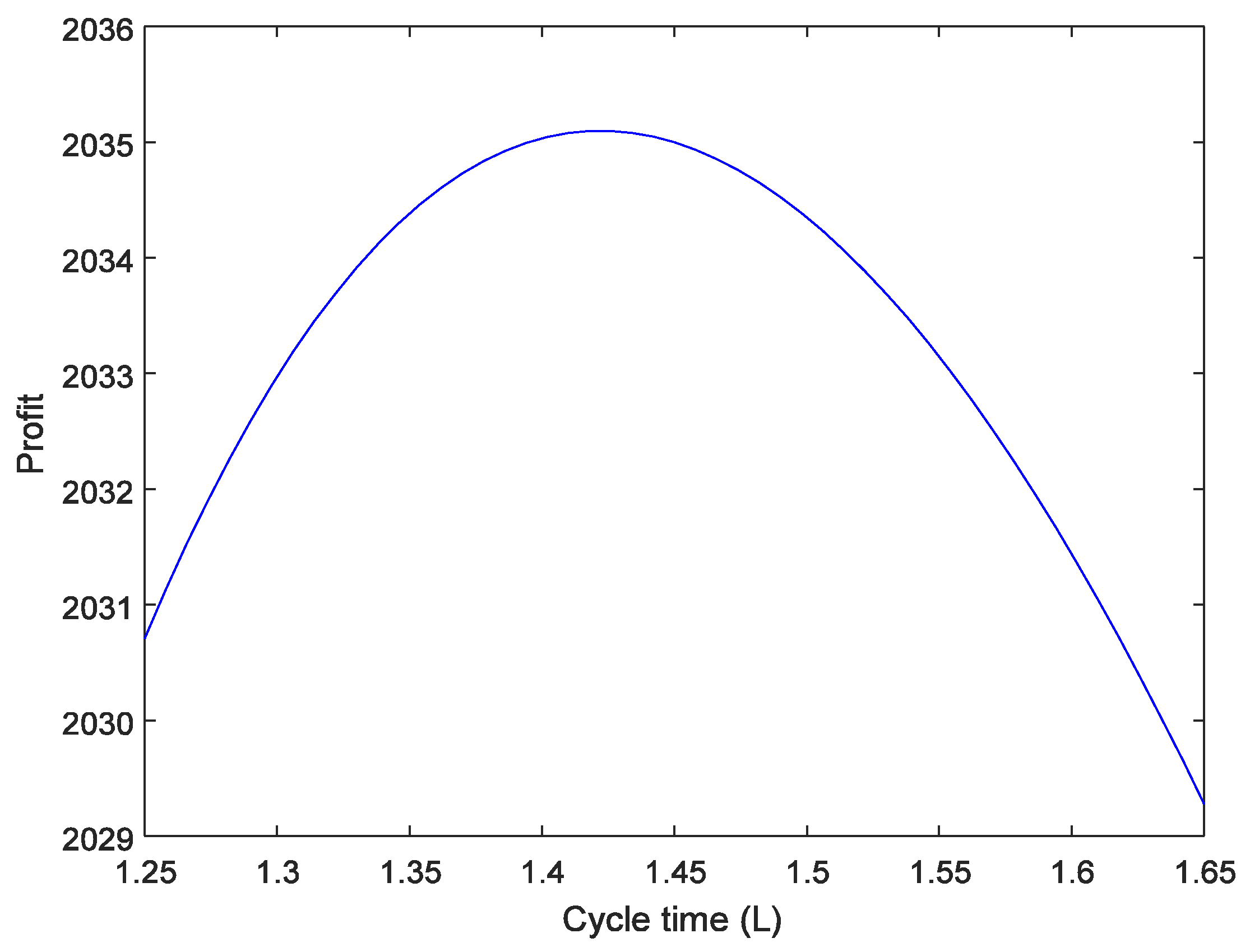
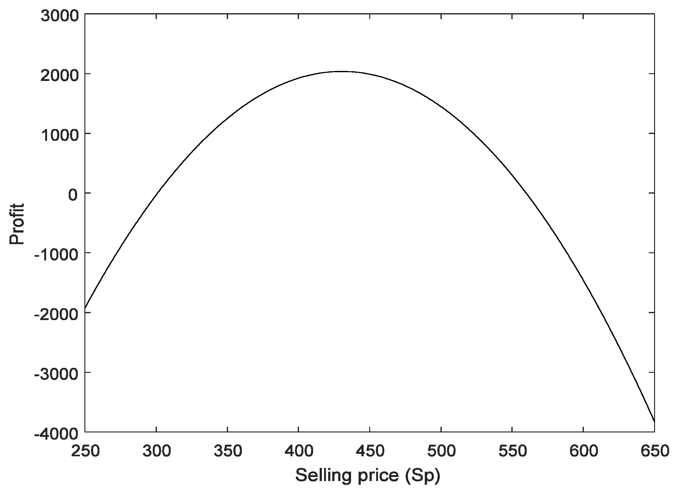
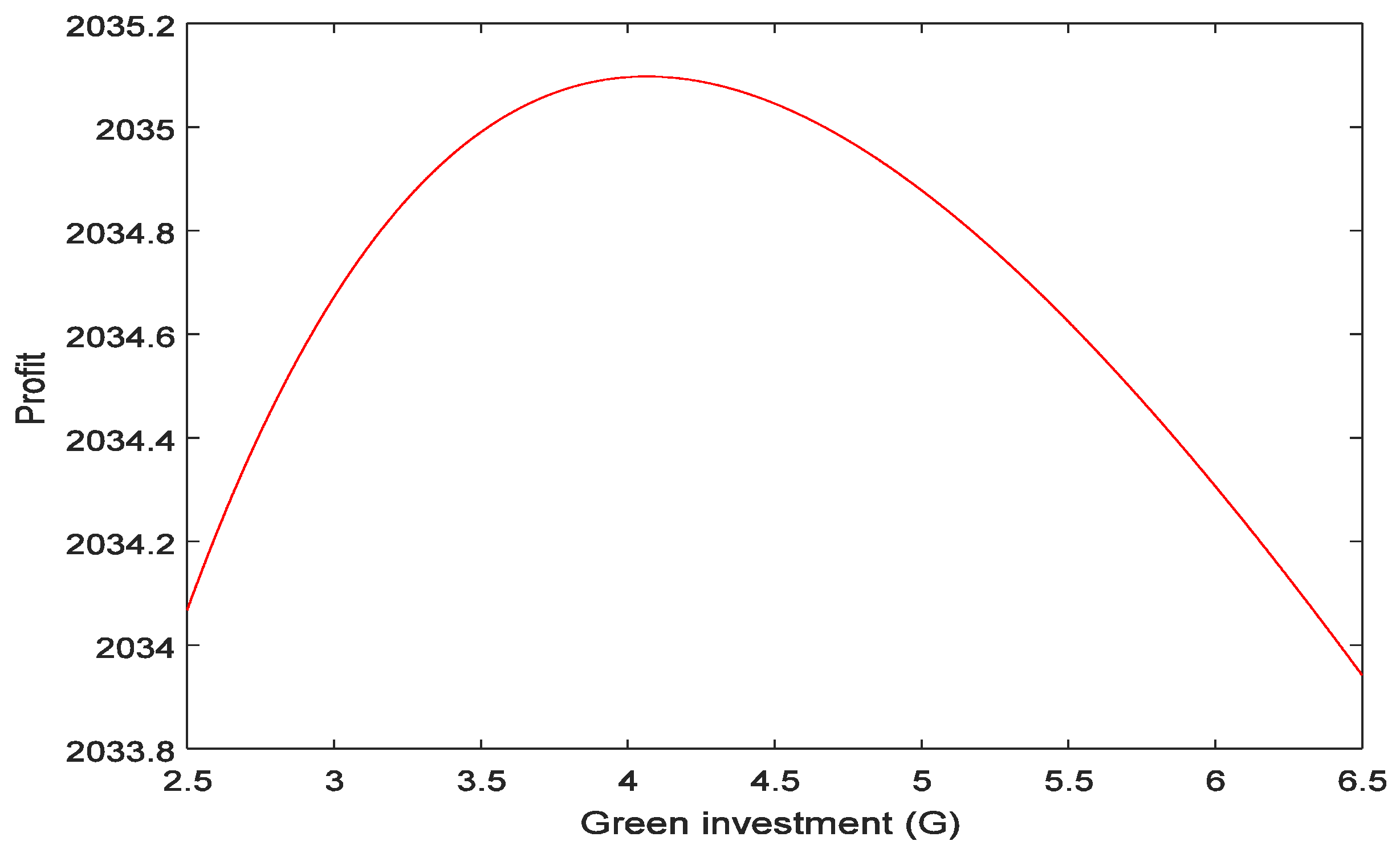
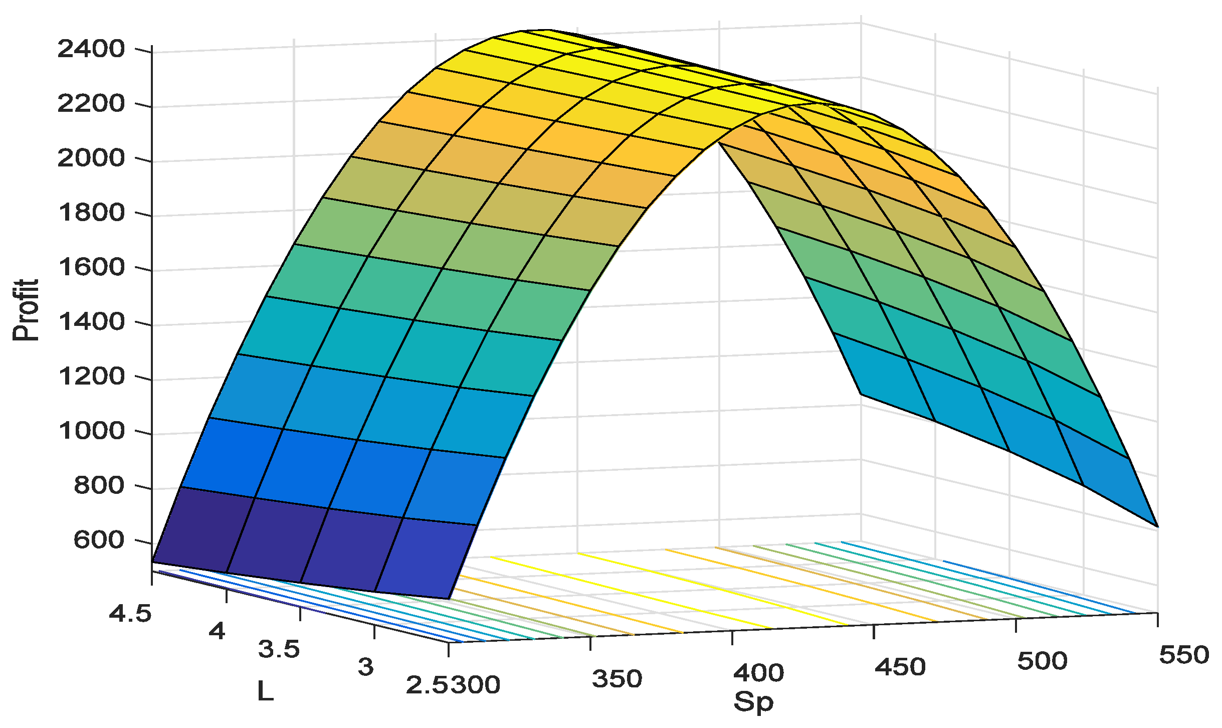
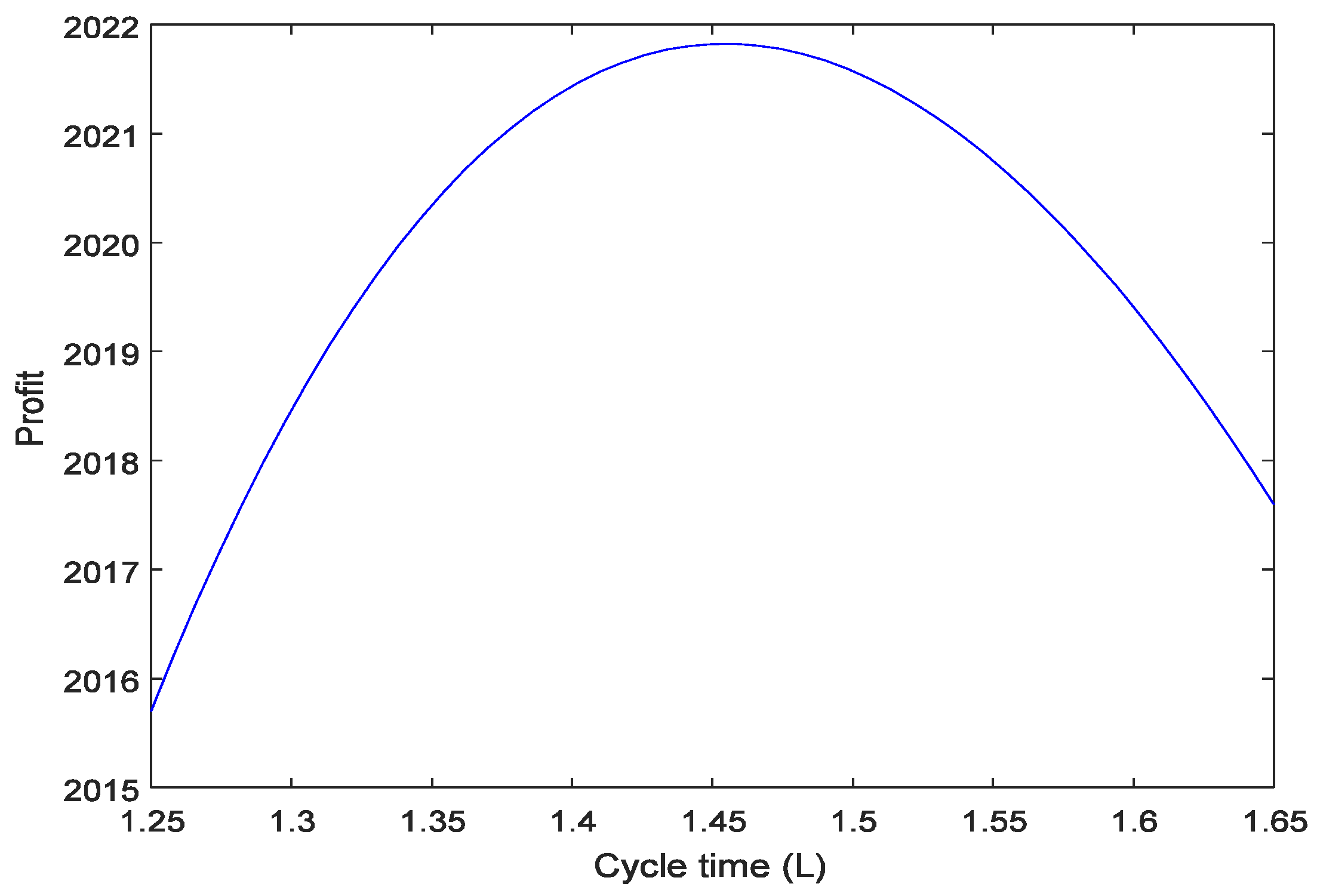
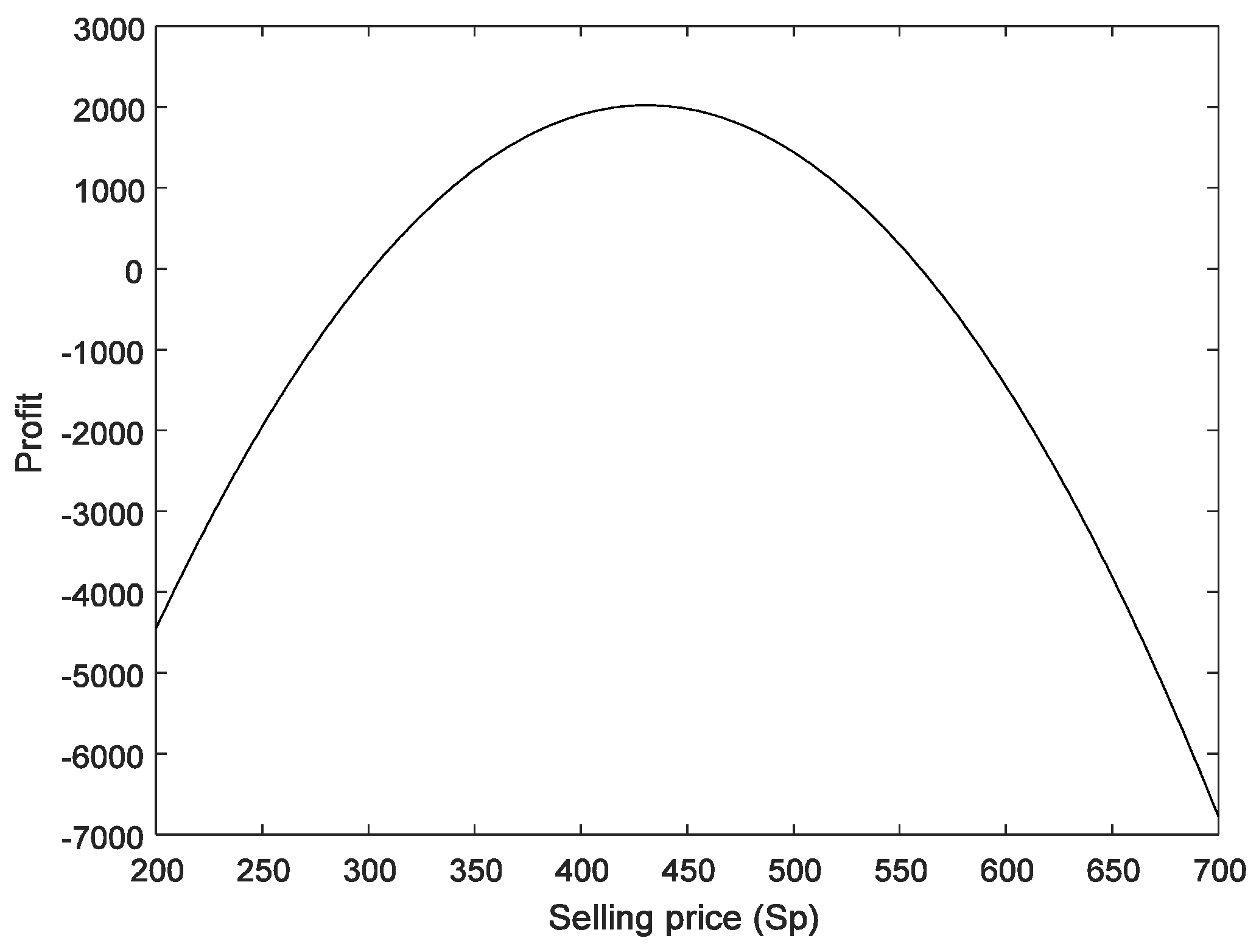
4. Numerical Illustrations and Discussions

This section presents a solution algorithm (Algorithm 1) with some numerical examples continued by a sensitivity analysis, and, finally, we discuss managerial insights regarding the results of this study.

4.1. Algorithm

Algorithm 1. (Solution Algorithm)

Step 1.  Initialize Lingo 17 software to solve this problem, with the preliminary factors. (For example, consider all the mentioned parametric values of Example 1.)

Step 2.  Set the step size of $s_p={\varpi }_1, G={\varpi }_2, L={\varpi }_3$ (say).

Step 3.  Initialize sp = 0, G = 0, L = 0.

Step 4.  Derive the critical points L*, sp*, and G* from Equations (20), (24), and (28).

Step 5.  If G < 0, then contemplate G = 0, and go to Step 7, or else follow Step 6.

Step 6.  Repeat Step 4 until the stable values of sp, L, and G are obtained. Let us guess this value G = G1.

Step 7.  G = Min [G1, Gmax].

Step 8.  Store the optimal value of critical points sp*, L*, and G*.

Step 9.  Now, check the sufficient condition for G* (when sp and L fixed) by following a similar procedure as stated in Corollary 1.

Step 10.  If Step 9 is satisfied, then evaluate at critical points; otherwise, the solution is not feasible.

Step 11.  Stop.

4.2. Numerical Examples

Example 1. 

A set of parametric values concerning the costs, emissions, demand function, deterioration, and investments of the inventory system are collected from a business firm as follows:

g = 60, g₁ = 60, L₁ = 0.3 year, h = 0.1, q = 0.5, γ = $11.526, j = 4, σ = 0.25, ϕ₁ = 0.2, ϕ₂ = 0.25, r = 0.2, A_oc = $800, p_rc = $200, c_scr = $2, h₁ = $6, h₂ = $7, m = 2, n = 1, u = $0.03, v = $0.02, d_st = 100, w_p = 3, n_t = 2, F_ct = $0.4, t_cp = 30, T_c = $1.5, c_fh = 0.8, c_vh = 0.7, n_g = 25, e = 0.6, π = 0.02, and Y = 0.6.

Now, from Corollary 1, one finds $\frac{1}{L^{*}}{\mathsf{\Omega }}_1{\left\{{\varphi }_{1}p\left(\gamma \right)\right\}}^2\left[{\varphi }_{1}p\left(\gamma \right)L^{*}-1\right]+4{\mathsf{\Omega }}_3{\left\{{\varphi }_{1}p\left(\gamma \right)\right\}}^3=114563.6$ and $\frac{2}{L^{*}{}^3}{\mathsf{\Omega }}_2=-257.2964$, which implies that $\frac{1}{L^{*}}{\mathsf{\Omega }}_1{\left\{{\varphi }_{1}p\left(\gamma \right)\right\}}^2\left[{\varphi }_{1}p\left(\gamma \right)L^{*}-1\right]+4{\mathsf{\Omega }}_3{\left\{{\varphi }_{1}p\left(\gamma \right)\right\}}^3>\frac{2}{L^{*}{}^3}{\mathsf{\Omega }}_2$. Thus, employing Corollary 1 to Proposition 1, one has, from Equation (22),${\left[\frac{{\partial }^2\alpha }{\partial L^2}\right]}_{L=L^{*}}=-114820.9 < 0$, which satisfies Proposition 1.

Now, similarly from Corollary 2, one can exploit the result as $\left[\pi Y^2{\Delta }_6\left(1-Y{G}^{*}\right)+6{\pi }^2{Y}^3{\Delta }_7{G}^{*}-2{\pi }^2{Y}^2{\Delta }_7\left(1+Y^2{G}^{*}{}^2\right)\right]=1.474710$, which is greater than zero, to prove Proposition 4. Thus, according to Proposition 4, Equation (29) provides a negative result for the maximum profit of the function ${\left[\frac{{\partial }^2\alpha }{\partial G^2}\right]}_{G=G^{*}}=-1.036963 < 0$. All the conditions are satisfied and, hence, this ensures the optimality of the profit. Therefore, analyzing these data in Lingo software, the optimal solutions are cycle time L* = 1.422 years, selling price s_p* = $430.480, green investment per unit G* = $4.064, and profit α* = $2035.097.

Figure 2, Figure 3, Figure 4, Figure 5 and Figure 6 show the concavity of the profit function with regard to the decision variables of Example 1.

Example 2. 

Now, we have a case when the retailer does not want to take the trouble of transporting items. This means that the customers must bring the products by themselves. In this situation, there will be no carbon emissions for transportation.

For this case, simply ignoring the parameters related to transportation and taking the other parameters as in Example 1, we obtain the following optimal solutions: cycle time L* = 3.57 years, selling price s_p* = $432.270, green investment per unit G* = $3.734, and profit α* = $2428.193.

Figure 7 shows the concavity of the profit function with regard to the decision variables of Example 2.

Example 3. 

For the case when the retailer does not invest in green technology, taking G = 0 and the other parameters as in Example 1, the following optimal solutions are found: cycle time L* = 1.455 years, selling price s_p* = $430.827, and profit α* = $2021.824.

Figure 8 and Figure 9 show the concavity of the profit function with regard to the decision variables of Example 3.

Example 4. 

For the same parametric values as in Example 1 except with j (coefficient of customer’s choice for low carbon emissions), the optimal solutions are provided in

Table 1. Influences of customer’s choice for low carbon emissions on the retailer’s decision.

j	L*	sp*	G*	λ*	Profit (α*)
0	1.448	430.673	1.242	0.0105	2022.424
2	1.434	430.542	3.186	0.0170	2028.214
4	1.422	430.480	4.064	0.0183	2035.097
10	1.386	430.304	5.414	0.0192	2057.208
15	1.355	430.130	6.059	0.0195	2076.320
21	1.317	429.876	6.613	0.0196	2099.737

.

When j = 0, i.e., customers are not concerned about eco-friendly products, the green investment G is much less. With the increase in j, the retailer extends the green investment G. Thus, the emission reduction percentage (λ) increases, for which the customer demand as well as the profit increases.

4.3. Sensitivity Analysis

In this section, a sensitivity analysis was performed in to show the consequences of the esteemed parameter by changing its value from −20% to +20%, provided in

Table 2. Sensitivity analysis with respect to different parameters.

Parameter	% Change	sp*	G*	L*	α*	% Changes in
						sp*	G*	L*	α*
Tc	−20	427.168	4.061	1.296	2071.114	−0.77	−0.08	−8.87	1.77
	−10	428.691	4.061	1.353	2055.223	−0.42	−0.07	−4.88	0.99
	10	431.913	4.069	1.480	2017.875	0.33	0.12	4.08	−0.85
	20	433.239	4.074	1.535	2001.093	0.64	0.25	7.97	−1.67
wp	−20	430.928	3.999	1.580	2098.410	0.10	−1.59	11.08	3.11
	−10	430.699	4.033	1.495	2066.155	0.05	−0.77	5.14	1.53
	10	430.273	4.095	1.358	2005.108	−0.05	0.76	−4.47	−1.47
	20	430.075	4.124	1.302	1976.047	−0.09	1.48	−8.42	−2.90
ϕ1	−20	430.515	4.064	1.424	2035.563	0.008	−0.01	0.16	0.02
	−10	430.498	4.064	1.423	2035.330	0.004	−0.002	0.08	0.01
	10	430.463	4.065	1.421	2034.865	−0.004	0.02	−0.06	−0.01
	20	430.446	4.065	1.420	2034.632	−0.008	0.03	−0.14	−0.02
ϕ2	−20	430.480	4.064	1.422	2035.098	0.00	0.008	0.01	0.00
	−10	430.480	4.064	1.422	2035.098	0.00	0.008	0.01	0.00
	10	430.480	4.064	1.422	2035.097	0.00	0.008	0.01	0.00
	20	430.480	4.064	1.422	2035.097	0.00	0.008	0.01	0.00
r	−20	434.957	3.920	1.796	1935.716	1.04	−3.54	26.29	−4.88
	−10	432.900	3.986	1.613	1984.356	0.56	−1.92	13.41	−2.49
	10	427.412	4.164	1.218	2088.789	−0.71	2.47	−14.31	2.64
	20	422.903	4.309	0.986	2147.114	−1.76	6.03	−30.63	5.50
σ	−20	417.921	4.207	1.244	2365.504	−2.92	3.53	−12.54	16.24
	−10	424.024	4.138	1.330	2203.151	−1.50	1.81	−6.49	8.26
	10	437.084	3.989	1.519	1868.429	1.53	−1.85	6.85	−8.19
	20	444.772	3.899	1.638	1682.148	3.32	−4.06	15.19	−17.34
h1	−20	429.887	4.069	1.423	2060.422	−0.14	0.13	0.07	1.24
	−10	430.183	4.067	1.423	2047.749	−0.07	0.07	0.04	0.62
	10	430.779	4.062	1.422	2022.469	0.07	−0.05	−0.01	−0.62
	20	431.078	4.059	1.422	2009.863	0.14	−0.11	−0.03	−1.24
h2	−20	430.356	4.067	1.418	2035.468	−0.03	0.06	−0.31	0.02
	−10	430.418	4.065	1.420	2035.282	−0.01	0.04	−0.15	0.01
	10	430.542	4.063	1.424	2034.914	0.01	−0.02	0.17	−0.01
	20	430.603	4.062	1.427	2034.730	0.03	−0.05	0.33	−0.02
e	−20	427.754	4.077	1.306	2057.582	−0.63	0.32	−8.17	1.10
	−10	429.251	4.069	1.368	2045.652	−0.29	0.13	−3.78	0.52
	10	431.597	4.061	1.473	2024.925	0.26	−0.09	3.60	−0.50
	20	432.621	4.058	1.522	2015.092	0.50	−0.15	7.02	−0.98
nt	−20	431.528	4.017	1.593	2084.431	0.24	−1.16	12.05	2.42
	−10	431.033	4.040	1.506	2060.373	0.13	−0.59	5.91	1.24
	10	429.947	4.087	1.352	2012.143	−0.12	0.57	−4.92	−1.13
	20	429.133	4.120	1.261	1979.473	−0.31	1.38	−11.34	−2.73
Y	−20	430.489	4.615	1.423	2034.130	0.002	13.56	0.07	−0.05
	−10	430.484	4.321	1.422	2034.656	0.001	6.31	0.03	−0.02
	10	430.477	3.839	1.422	2035.474	−0.001	−5.53	−0.01	0.02
	20	430.474	3.640	1.422	2035.799	−0.001	−10.42	−0.03	0.03

.

Some observations can be made from the sensitivity table, as follows.

(1)

When the carbon emission tax (T_c) increases, the selling price (s_p) of the products increases. Consequently, this also intensifies the green investment (G) and the replenishment cycle (L). In contrast, the profit of the system (α) decreases. In an increasing emission tax situation, the retailer must invest more in controlling the emissions and, thus, increases the selling price to compensate for these expenses. Then, the total lot size requires more time to sell the products, resulting in an increased replenishment cycle; however, this strategy declines the retailer’s profit.

(2)

When the product weight (w_p) increases, the decision for green technology investment also increases to anticipate the increasing emissions from extra fuel in the transportation system. Simultaneously, the selling price and the replenishment cycle decrease. The increasing costs will consequently diminish the retailer’s profit.

(3)

Suppose the deterioration rate of perfect items (ϕ₁) increases. This will decrease the selling price, replenishment cycle, and profit, while green technology investment is relatively constant. The increasing deterioration rate decreases the total profit due to increasing product loss. Due to the risk of deterioration, the retailer decreases the selling price to sell the products quickly to avoid this unavoidable circumstance. However, the change in the deterioration rate of the imperfect items (ϕ₂) does not change the decision variables and the total profit.

(4)

When the discount rate (r) for the defective items increases, the selling price decreases while the profit for the retailer increases. The discount rate and selling price boost the sales and, as a result, this instantly penetrates the profit of the retailer. However, as the discount is a catalyst to increase sales, the retailer invests more in green technology.

(5)

When the amount of imperfect portion (σ) increases, this simultaneously increases the selling price and the replenishment cycle. In contrast, this significantly decreases the retailer’s total profit and highly decreases the need for green investment. An increase in the percentage of imperfect items causes a major loss for the retailer; hence, the retailer may increase the selling price to reduce the impact.

(6)

The holding cost for the perfect items and imperfect items provides a similar sort of observation, except for the replenishment cycle. However, the effect is higher from the perfect items as their percentage is also larger. When per unit holding cost increases, the retailer’s total profit decreases, and, again, the retailer may increase the selling price to reduce the impact.

(7)

When the unit GHG emissions of the truck fuel (e) increase, this results in a decrease in the total profit as it causes higher costs. This also greatly increases the replenishment cycle to reduce the delivery frequency, which will curb the total emissions.

(8)

The profit also declines due to an increase in the number of trips (n_t). In the real case, when the retailer is bound to increase the trip number, this intensifies the transportation costs and the number of carbon emissions; therefore, the retailer needs to invest more in green technology to curb the emissions. In the end, it results in a decrease in profit.

(9)

As we expected, the efficiency of greener technology (Y) helps the retailer to invest less in green technology. However, it does not increase profit significantly. The selling price and replenishment cycle also remain constant.

4.4. Managerial Insights

Important insights that would be helpful for retail businesses can be drawn from this study for the managers of industries. This study showed that the rate of imperfect items had a significant effect on the total profit, which is similar to results found in previous research, such as Vishkaei et al. [16] and Yu and Hsu [17]. Hence, a retailer must keep the rate as low as possible. Careful monitoring and possible collaboration to improve the supplier’s quality performance may help to reduce the impact. In another way, this study recommends managers to offer a discount that is compatible with the other attributes (e.g., the product weight, number of trips, carbon tax, and holding cost) on imperfect items to enhance the sales and, consequently, the profit.

By using the proposed model, a manager can easily determine the optimum selling price to achieve a safe margin in profit. An optimization in the selling price provides an intensification in the demand of the customers and, consequently, to the profits, as seen in Tiwari et al. [36] and Khan et al. [37]. Specifically, this study suggests that the manager should know the situations when the selling price needs to be increased to be compatible with the increase in the rate of imperfect items, emission tax, holding cost, and fuel emission rate.

Green technology investment always provides some relaxation to the managers in curbing environmental effects and attracting more customers toward the business, as shown in Gao et al. [2] and Lou et al. [7]. By implementing the model, a manager can easily understand the optimal investment in green technology. The decision is affected by emission-related parameters, such as the level of the carbon tax, number of deliveries, and product weight; hence, managers must be able to anticipate these parameters. However, the retailer can make the decision for the business when the investment needs to be reduced based on investment efficiency and the increasing rate of imperfect items.

This study comprises preservation technology to maintain the deterioration rate of the inventory. This technology helps managers to preserve the quality of the products to the original conditions, thus, minimizing the loss. Managers can have a sense of how much to invest and the optimum time to curb the deterioration of the products.

5. Conclusions

In this research, we studied a sustainable inventory model with imperfect products, deterioration, and controllable emissions. To make the business more profitable, preservation technology was used to control the deterioration of the products. Theories were developed to support the validity of the model, and numerical illustrations were provided. This study identified several parameters that highly affected the total profit, selling price, green technology investment, and replenishment cycle.

An inspection process was introduced to segregate the imperfect products from the perfect ones. The proposed model considered different realistic holding costs for perfect and imperfect items, which included a fixed and variable part for different types of products. From the proposed framework, it is clear how the inspection process provides benefits from sorting the imperfect goods from the perfect ones. A discount policy was introduced to stimulate the sales of imperfect products, which was outstandingly effective.

This study provides a clear idea of the impacts of a green degree in environmentally conscious customer choices for the purchase of sustainable inventory. These impacts will have a positive effect to promote the green awareness of customers in their social daily life, and when more customers choose high green-degree products, the supplier is encouraged to make those products, which will reduce GHGs, including CO₂. This result elucidates how a suitable green investment can curb the growing carbon emissions in the environment. In the long run, these changes will help to recover the climate and provide other positive impacts, such as improving people’s health.

Certain limitations of the proposed model are also noticeable. It considered transportation as the sole source of carbon emissions; however, future research could incorporate other sources of emissions. The model can be extended in several ways by implementing other carbon-curbing regulations, e.g., cap policies and cap-and-trade policies. A continuous inspection process can be placed irrespective of a single inspection process in a future study. The changes in the demand pattern, e.g., fuzzy demand and stochastic demand, are another possible scope of extensions for this proposed model. Another interesting extension could also include whether the retailer offers a credit policy to its customers.

References

- Intergovernmental Panel on Climate Change (IPCC). Climate Change 2007: The Fourth Assessment Report of the Intergovernmental Panel on Climate Change; Cambridge University Press: Cambridge, UK, 2007. [Google Scholar]
- Gao, X.; Zheng, H.; Zhang, Y.; Golsanami, N. Tax policy, environmental concern and level of emission reduction. Sustainability 2019, 11, 1047. [Google Scholar] [CrossRef]
- Mishra, U.; Wu, J.Z.; Chiu, A.S.F. Effects of carbon-emission and setup cost reduction in a sustainable electrical energy supply chain inventory system. Energies 2019, 12, 1226. [Google Scholar] [CrossRef]
- Mishra, U.; Wu, J.Z.; Tsao, Y.C.; Tseng, M.L. Sustainable inventory system with controllable non-instantaneous deterioration and environmental emission rates. J. Clean. Prod. 2020, 244, 118807. [Google Scholar] [CrossRef]
- Sarkar, B.; Ahmed, W.; Choi, S.B.; Tayyab, M. Sustainable inventory management for environmental impact through partial backordering and multi-trade-credit-period. Sustainability 2018, 10, 4761. [Google Scholar] [CrossRef]
- Tiwari, S.; Daryanto, Y.; Wee, H.M. Sustainable inventory management with deteriorating and imperfect quality items considering carbon emissions. J. Clean. Prod. 2018, 192, 281–292. [Google Scholar] [CrossRef]
- Lou, G.X.; Xia, H.Y.; Zhang, J.Q.; Fan, T.J. Investment strategy of emission-reduction technology in a supply chain. Sustainability 2015, 7, 10684–10708. [Google Scholar] [CrossRef]
- He, Y.; Huang, H. Optimizing inventory and pricing policy for seasonal deteriorating products with preservation technology investment. J. Ind. Eng. 2013, 793568, 1–7. [Google Scholar] [CrossRef]
- Mishra, U.; Tijerina-Aguilera, J.; Tiwari, S.; Cárdenas-Barrón, L.E. Retailer’s joint ordering, pricing, and preservation technology investment policies for a deteriorating item under permissible delay in payments. Math. Probl. Eng. 2018, 6962417, 1–14. [Google Scholar] [CrossRef]
- Saltveit, M.E. Effect of ethylene on quality of fresh fruits and vegetables. Postharvest Biol. Technol. 1999, 15, 279–292. [Google Scholar] [CrossRef]
- Barry, C.S.; Giovannoni, J.J. Ethylene and Fruit Ripening. J. Plant Growth Regul. 2007, 26, 143–159. [Google Scholar] [CrossRef]
- Kazemi, N.; Abdul-Rashid, S.H.; Ghazilla, R.A.R.; Shekarian, E.; Zanoni, S. Economic order quantity models for items with imperfect quality and emission considerations. Int. J. Syst. Sci. Oper. Logist. 2018, 5, 99–115. [Google Scholar] [CrossRef]
- Daryanto, Y.; Christata, B.R.; Kristiyani, I.M. Retailer’s EOQ model considering demand and holding cost of the defective items under carbon emission tax. IOP Conf. Ser. Mater. Sci. Eng. 2020, 847, 012012. [Google Scholar] [CrossRef]
- Rosenblatt, M.J.; Lee, H.L. Economic production cycles with imperfect production processes. IIE Trans. 1986, 18, 48–55. [Google Scholar] [CrossRef]
- Porteus, E.L. Optimal lot sizing, process quality improvement and setup cost reduction. Oper. Res. 1986, 34, 137–144. [Google Scholar] [CrossRef]
- Vishkaei, B.M.; Niaki, S.T.A.; Farhangi, M.; Rashti, M.E.M. Optimal lot sizing in screening processes with returnable defective items. J. Ind. Eng. Int. 2014, 10, 70. [Google Scholar] [CrossRef]
- Yu, H.F.; Hsu, W.K. An integrated inventory model with immediate return for defective items under unequal-sized shipments. J. Ind. Prod. Eng. 2017, 34, 70–77. [Google Scholar] [CrossRef]
- Salameh, M.K.; Jaber, M.Y. Economic production quantity model for items with imperfect quality. Int. J. Prod. Econ. 2000, 64, 59–64. [Google Scholar] [CrossRef]
- Goyal, S.K.; Huang, C.K.; Chen, K.C. A simple integrated production policy of an imperfect item for vendor and buyer. Prod. Plan. Control 2003, 14, 596–602. [Google Scholar] [CrossRef]
- Maddah, B.; Jaber, M.Y. Economic order quantity for items with imperfect quality: Revisited. Int. J. Prod. Econ. 2008, 112, 808–815. [Google Scholar] [CrossRef]
- Teng, H.M.; Hsu, P.H. Revisit economic ordering strategy for items with imperfect quality and backordering. Int. J. Manag. Enterp. Dev. 2013, 12, 251–262. [Google Scholar] [CrossRef]
- Lin, T.Y. An economic order quantity with imperfect quality and quantity discounts. App. Math. Model. 2010, 34, 3158–3165. [Google Scholar] [CrossRef]
- Wahab, M.I.M.; Jaber, M.Y. Economic order quantity model for items with imperfect quality, different holding costs, and learning effects: A note. Comput. Ind. Eng. 2010, 58, 186–190. [Google Scholar] [CrossRef]
- Alamri, A.A.; Harris, I.; Syntetos, A.A. Efficient inventory control for imperfect quality items. Eur. J. Oper. Res. 2016, 254, 92–104. [Google Scholar] [CrossRef]
- Shaikh, A.A.; Khan, M.A.; Panda, G.C.; Konstantaras, I. Price discount facility in an EOQ model for deteriorating items with stock-dependent demand and partial backlogging. Int. Transact. Oper. Res. 2019, 26, 1365–1395. [Google Scholar] [CrossRef]
- Jaggi, C.K.; Goel, S.K.; Mittal, M. Economic order quantity model for deteriorating items with imperfect quality and permissible delay on payment. Int. J. Ind. Eng. Comput. 2011, 2, 237–248. [Google Scholar] [CrossRef]
- Jaggi, C.K.; Mittal, M.; Khanna, A. Effects of inspection on retailer’s ordering policy for deteriorating items with time-dependent demand under inflationary conditions. Int. J. Syst. Sci. 2013, 44, 1774–1782. [Google Scholar] [CrossRef]
- Moussawi-Haidar, L.; Salameh, M.; Nasr, W. Effect of deterioration on the instantaneous replenishment model with imperfect quality items. Appl. Math. Model. 2014, 38, 5956–5966. [Google Scholar] [CrossRef]
- Dye, C.Y. The effect of preservation technology investment on a non-instantaneous deteriorating inventory model. Omega 2013, 41, 872–880. [Google Scholar] [CrossRef]
- Mashud, A.H.M.; Hasan, M.R.; Wee, H.M.; Daryanto, Y. Non-instantaneous deteriorating inventory model under the joined effect of trade-credit, preservation technology and advertisement policy. Kybernetes 2020, 49, 1645–1674. [Google Scholar] [CrossRef]
- Mashud, A.H.M.; Wee, H.M.; Huang, C.V. Preservation technology investment, trade credit and partial backordering model for a non-instantaneous deteriorating inventory. RAIRO-Oper. Res. 2019, in press. [Google Scholar] [CrossRef]
- Hsu, P.H.; Wee, H.M.; Teng, H.M. Preservation technology investment for deteriorating inventory. Int. J. Prod. Econ. 2010, 124, 388–394. [Google Scholar] [CrossRef]
- Dye, C.Y.; Yang, C.T.; Wu, C.C. Joint dynamic pricing and preservation technology investment for an integrated supply chain with reference price effects. J. Oper. Res. Soc. 2017, 69, 811–824. [Google Scholar] [CrossRef]
- Li, G.; He, X.; Zhou, J.; Wu, H. Pricing, replenishment and preservation technology investment decisions for non-instantaneous deteriorating items. Omega 2019, 84, 114–126. [Google Scholar] [CrossRef]
- Mashud, A.H.M. A deteriorating inventory model with different types of demand and fully backlogged shortages. Int. J. Logis. Sys. Manag. 2020, 36, 16–45. [Google Scholar] [CrossRef]
- Tiwari, S.; Cárdenas-Barrón, L.E.; Goh, M.; Shaikh, A.A. Joint pricing and inventory model for deteriorating items with expiration dates and partial backlogging under two-level partial trade credits in supply chain. Int. J. Prod. Econ. 2018, 200, 16–36. [Google Scholar] [CrossRef]
- Khan, M.A.; Shaikh, A.A.; Panda, G.C.; Konstantaras, I.; Taleizadeh, A.A. Inventory system with expiration date: Pricing and replenishment decisions. Comput. Ind. Eng. 2019, 132, 232–247. [Google Scholar] [CrossRef]
- Mishra, V.K.; Singh, L.S.; Kumar, R. An inventory model for deteriorating items with time-dependent demand and time-varying holding cost under partial backlogging. J. Ind. Eng. Int. 2013, 9, 1–5. [Google Scholar] [CrossRef]
- Sicilia, J.; González-De-la-Rosa, M.; Febles-Acosta, J.; Alcaide-López-de-Pablo, D. An inventory model for deteriorating items with shortages and time-varying demand. Int. J. Prod. Econ. 2014, 155, 155–162. [Google Scholar] [CrossRef]
- Tiwari, S.; Wee, H.M.; Sarkar, S. Lot-sizing policies for defective and deteriorating items with time-dependent demand and trade credit. Eur. J. Ind. Eng. 2017, 11, 683–703. [Google Scholar] [CrossRef]
- Mashud, A.H.M.; Wee, H.M.; Huang, C.V.; Wu, J.-Z. Optimal replenishment policy for deteriorating products in a newsboy problem with multiple just-in-time deliveries. Mathematics 2020, 8, 1981. [Google Scholar] [CrossRef]
- Saren, S.; Sarkar, B.; Bachar, R.K. Application of various price-discount policy for deteriorated products and delay-in-payments in an advanced inventory model. Inventions 2020, 5, 50. [Google Scholar] [CrossRef]
- Hasan, M.R.; Mashud, A.H.M.; Daryanto, Y.; Wee, H.M. A non-instantaneous inventory model of agricultural products considering deteriorating impacts and pricing policies. Kybernetes 2020, in press. [Google Scholar] [CrossRef]
- Khakzad, A.; Gholamian, M.R. The effect of inspection on deterioration rate: An inventory model for deteriorating items with advance payment. J. Clean. Prod. 2020, 254, 120117. [Google Scholar] [CrossRef]
- Bonney, M.; Jaber, M.Y. Environmentally responsible inventory models: Non-classical models for a non-classical era. Int. J. Prod. Econ. 2011, 133, 43–53. [Google Scholar] [CrossRef]
- Shi, Y.; Zhang, Z.; Chen, S.C.; Cárdenas-Barrón, L.E.; Skouri, K. Optimal replenishment decisions for perishable products under cash, advance, and credit payments considering carbon tax regulations. Int. J. Prod. Econ. 2020, 223, 107514. [Google Scholar] [CrossRef]
- Taleizadeh, A.A.; Hazarkhani, B.; Moon, I. Joint pricing and inventory decisions with carbon emission considerations, partial backordering and planned discounts. Ann. Oper. Res. 2020, 290, 95–113. [Google Scholar] [CrossRef]
- Daryanto, Y.; Wee, H.M.; Widyadana, G.A. Low carbon supply chain coordination for imperfect quality deteriorating items. Mathematics 2019, 7, 234. [Google Scholar] [CrossRef]
- Yang, D.; Xiao, T.; Huang, J. Dual-channel structure choice of an environmental responsibility supply chain with green investment. J. Clean. Prod. 2019, 210, 134–145. [Google Scholar] [CrossRef]
- Taleizadeh, A.A.; Alizadeh-Basban, N.; Sarker, B.R. Coordinated contracts in a two-echelon green supply chain considering pricing strategy. Comput. Ind. Eng. 2018, 124, 249–275. [Google Scholar] [CrossRef]
- Mishra, U.; Wu, J.Z.; Sarkar, B. Optimum sustainable inventory management with backorder and deterioration under controllable carbon emissions. J. Clean. Prod. 2021, 279, 123699. [Google Scholar] [CrossRef]
- Datta, T.K. Effect of green technology investment on a production-inventory system with carbon tax. Adv. Oper. Res. 2017, 4834839, 1–12. [Google Scholar] [CrossRef]