Variational Inference over Nonstationary Data Streams for Exponential Family Models †
by
 , , , and
Andrés R. Masegosa
1,* ,
,
Darío Ramos-López
2,
Antonio Salmerón
1,
Helge Langseth
3 and
Thomas D. Nielsen
4 1
Department of Mathematics and Center for Development and Transfer of Mathematical Research to Industry (CDTIME), University of Almería, 04120 Almería, Spain
2
Department of Applied Mathematics, Materials Science and Engineering, and Electronic Technology, Rey Juan Carlos University, 28933 Móstoles, Spain
3
Department of Computer Science, Norwegian University of Science and Technology, 7491 Trondheim, Norway
4
Department of Computer Science, Aalborg University, 9220 Aalborg, Denmark
*
Author to whom correspondence should be addressed.
†
This paper is an extended version of our previous work “Bayesian models of data streams with hierarchical power priors”, presented at the International Conference on Machine Learning 2017 Conference.
Mathematics 2020, 8(11), 1942; https://doi.org/10.3390/math8111942
Submission received: 8 October 2020
/
Revised: 26 October 2020
/
Accepted: 27 October 2020
/
Published: 3 November 2020
(This article belongs to the Section Probability and Statistics)
Abstract
:In many modern data analysis problems, the available data is not static but, instead, comes in a streaming fashion. Performing Bayesian inference on a data stream is challenging for several reasons. First, it requires continuous model updating and the ability to handle a posterior distribution conditioned on an unbounded data set. Secondly, the underlying data distribution may drift from one time step to another, and the classic i.i.d. (independent and identically distributed), or data exchangeability assumption does not hold anymore. In this paper, we present an approximate Bayesian inference approach using variational methods that addresses these issues for conjugate exponential family models with latent variables. Our proposal makes use of a novel scheme based on hierarchical priors to explicitly model temporal changes of the model parameters. We show how this approach induces an exponential forgetting mechanism with adaptive forgetting rates. The method is able to capture the smoothness of the concept drift, ranging from no drift to abrupt drift. The proposed variational inference scheme maintains the computational efficiency of variational methods over conjugate models, which is critical in streaming settings. The approach is validated on four different domains (energy, finance, geolocation, and text) using four real-world data sets.
1. Introduction
One core problem in Bayesian statistics is the computation of posterior probability over the parameters (and the latent variables) of a model given a data set. In most relevant cases, the computation of this posterior probability is not feasible and requires the use of approximate inference algorithms [1,2]. Moreover, in many real-life settings, the data set is not static but arrives sequentially, in a streaming fashion. Computing the Bayesian posterior probability over the parameters (and the latent variables) of a model, in this case, is even more challenging. First, it requires the ability to handle a posterior distribution conditioned on an unbounded data set. Secondly, the posterior probability has to be updated frequently, at every time step, imposing restrictions over the speed of computation of the posterior probability. Finally, the classical i.i.d. (independent and identically distributed, or data exchangeability) assumption does not hold because the underlying data distribution may drift/change from one time step to the next. This last issue is known in the machine learning literature as learning from data streams that exhibit concept drift [3] in the sense that the underlying generative process may contain both gradual and abrupt changes.
In this paper, we look at the common setting in many real-world problems, where data arrives as a sequence of (potentially large) batches. Specifically, each batch is associated with a new time step and the data points within a batch are assumed to be i.i.d. However, the underlying distribution generating the batches may change from one time step to the next. For illustration, in Section 6, we will apply a probabilistic topic model [4] to identify the main topics of research papers published over a sequence of years. New papers are submitted yearly; hence, every year, the probabilistic model must be updated to infer the topics of that year’s papers. One approach could be to discard all data from previous years, but that would result in a loss of relevant data that could potentially have been used to draw more accurate inferences about the current year’s topic distribution (research topics typically span multiple years). On the other hand, we also have to take into account that the underlying distribution of the papers may change from one year to the next following the development of the research field. As another example domain, we will model the financial profile of customers asking for a loan/mortgage from a financial institution [5]. In this example, we update the financial profile of the customers on a monthly basis while simultaneously keeping in mind that the occurrence of exogenous events (like an economic crisis) may strongly affect the customers and therefore induce a drift in the underlying data distribution. Other situations similar to the ones above arise in many different real-life settings.
Standard temporal models [6] have the potential to capture the underlying temporal dynamics of the data set. However, for the problems addressed in this paper, temporal models are not readily applicable. The reason for this is two-fold. First, the set of objects differs from one time step to the next. For example, a new set of papers is submitted to a conference every year. Thus, temporal modeling needs to be applied at the level of the parameters in the model, not at the objects themselves. Secondly, drift (both gradual and abrupt) in the underlying distributions is not easily modelled with a stationary transition model as would typically be the case in temporal models. Instead, we will employ an implicit transition model to model the temporal dynamics, thus sidestepping the problem of specifying an explicit stationary transition distribution.
The approach presented in this paper is applicable to domains that, at each time point, can be described by a conjugate exponential family model. These models are widely used in probabilistic modeling [7,8] and include popular models like latent Dirichlet allocation (LDA) models [4] to uncover the hidden topics in a text corpora, a mixture of (multivariate) Gaussian models to discover hidden clusters in data [9], and probabilistic principal component analysis for revealing a low-dimensional representation of the data [10]. See, for instance, [9,11,12] for detailed reviews and applications of these models in data mining and machine learning settings.
Exact Bayesian inference is intractable for the model-class proposed in this paper, partly due to the implicit transition model and partly due to the high dimensionality of the parameters/latent variables in the model. We therefore resort to approximate Bayesian inference methods, and owing to the potential real-time requirements imposed by the streaming domains, we focus on variational methods (see [13] for an introduction). Markov Chain Monte Carlo methods (MCMC) [1,2], although widely used in Bayesian statistics, are not as computationally efficient as variational methods, especially in the presence of large datasets or complex models [13]. Moreover, variational inference can be performed very efficiently in conjugate exponential family models by exploiting properties of this model family.
The rest of the paper is organized as follows. Section 2 discusses related works, and Section 3 introduces preliminaries relevant for the remainder of the paper. In Section 4, we introduce an implicit transition model that works as an off-the-self parameter transition scheme to model both gradual and abrupt changes in the data distribution. Section 5 positions the transition model in a hierarchical Bayesian setting to model the rate of change of the data stream as an unobserved mechanism. Section 5 also includes the derivation of an ad hoc variational inference algorithm [13], based on a novel lower-bound of the data log-likelihood function for the proposed model family (i.e., a conjugate exponential model with an implicit transition scheme). As a consequence, the proposed approximate inference scheme is deterministic and scales to large data streams. Section 6 empirically evaluates the appropriateness of our approach using both synthetic and real-life data (covering energy, finance, geolocation, and text data), showing promising results. We conclude in Section 7, where the main conclusions and future works are discussed.
2. Related Work
Making inferences from nonstationary data streams has been extensively studied in statistics. Time series models [14] is a classic example of models that could be assumed relevant for this problem, but as we are not dealing with temporal data (where the the same set of objects are observed at each time step), this model class is not applicable in our situation. Work by [15,16] is closer to ours, but these contributions focus on simpler model classes (like generalized linear models without latent variables), and due to this simplicity, they do not consider variational inference.
Methods for change point detection [17,18] are also related to our situation. However, where these methods consider abrupt changes in the data stream, our method is able to deal with both abrupt and smooth changes in the distribution. Additionally, the main focus of change point detection methods is the detection of points where the changes occur, while our goal is to have a statistical model that accurately models the data at each time step by continuously adapting the model parameters.
Learning from nonstationary data streams has also been extensively studied in the machine learning literature, especially in the context of classification and clustering [3,19,20,21]. One of the main techniques employed in this area has been exponential forgetting [22,23]. Here, each new observation is initially assigned a weight (or “importance”) equal to 1, followed by an exponential decrease of the weight at each subsequent time step. In this way, older observations are less relevant than newer ones when the model is learned, thereby accounting for potential drift in the data stream. The main problem with this approach is to quantify the so-called exponential forgetting rate, which is usually determined by the analyst on a trial-and-error basis. In the present work, we provide a sound approach based on Bayesian methods to automatically adjust the exponential forgetting rate and show the advantages of this strategy empirically.
Bayesian modeling of nonstationary data streams for general probabilistic inference has not been extensively studied so far. An online variational inference method, which exponentially forgets old data, was proposed by Honkela and Valpola [24], but similarly to [22,23], this approach suffers from the problem of setting the exponential forgetting rate. Another proposal, called population variational Bayes (PVB), was introduced by [25]. It builds directly on the stochastic variational inference (SVI) algorithm [26]. SVI assumes the existence of a fixed data set observed in a sequential manner and, in particular, that this data set has a known finite size. This is unrealistic when modeling data streams. PVB addresses the problem by using the frequentist notion of a population distribution, , which is assumed to generate the data stream by repeatedly sampling M data points at a time; here, M parameterizes the size of the population and helps control the variance of the population posterior. By artificially having high variance in the posterior (i.e., by choosing a small value for M), PVB is able to accommodate drift in the data set. Unfortunately, M must be specified by the user, and no clear rule exists for specifying it. Furthermore, McInerney et al., [25] shows that the optimal value for M may differ between data stream. The streaming variational Bayes (SVB) algorithm by [27] also tries to address Bayesian inference in data streams. SVB builds on a Bayesian recursive updating approach but does not provide a mechanism for dealing with concept drift. In Section 6, we will show that our proposed method, which does not rely on hyperparameters that are hard to tune, outperforms these closely related approaches on several real-world data sets.
The so-called power prior approach [28] has also been studied in the context of data aggregation for Bayesian modeling. Power priors provide a sound mechanism for Bayesian updating in light of new data and introduces partial forgetting of older observations. The approach enjoys nice theoretical properties [29] but depends on a hyperparameter (set by the analyst) to control the forgetting rate. Our work builds partially on the power prior model but extends this model with a Bayesian model of the forgetting mechanism, thereby dispensing of the analyst-specified hyperparameter.
A modeling approach based on time-series models for concept drift using implicit transition models was pursued by [30,31]. Unfortunately, the implicit transition model also depends on a hyperparameter determining the forgetting factor, which has to be manually set. Our work also partially builds on this approach and establishes novel connections between the implicit transition models [30,31], power priors [28], and exponential forgetting [22,23].
Many other contributions have proposed an ad hoc extension to specific statistical models in order to deal with nonstationary data streams [32,33], including dynamic extensions of latent Dirichlet allocation (LDA) models [34,35,36]. However, none are so far applicable to general conjugate exponential family models. Moreover, most of these contributions rely on complex and tailor-made inference mechanisms, instead of variational inference (which is well understood for conjugate exponential models).
3. Preliminaries
3.1. Conjugate Exponential Models
Let denote a set of observed variables, denote a set of latent variables, and denote the parameters of the model. Let also denote a hyperparameter vector.
We assume that the joint distribution of our statistical model factorizes into a product of local terms and a global term:
This kind of factorization is quite usual in many statistical models [26], for example, the case of the Bayesian mixture of Gaussian, where each latent variable is a categorical variable defining the component to which each data point belongs. We also consider the special case when there are no latent variables; this case would cover models like Bayesian linear regression. Figure 1a provides a graphical description of these model family in terms of probabilistic graphical models with plateau notation [11].
We further assume that the (conditional) distributions defining the statistical model belong to the conjugate exponential family [37]. This model family has been largely studied and covers a wide range of probability distributions such as multinomial, normal, gamma, Dirichlet, beta, etc. According to this assumption, the functional form of the conditional distribution of the local variables given the parameters has the well-known exponential family form [37]:
where the scalar functions and are the base measure and the log-normalizer, respectively, and the vector function is the sufficient statistics vector. Moreover, the prior distribution also belongs to the exponential family and has the following structure:
where the sufficient statistics are and the hyperparameter has two components , where the first component has the same dimension as and encodes the prior belief about the distribution over and the second component is a scalar and encodes the strength in our prior belief [38]. This second parameter is also known in the literature [39] as the equivalent sample size of the prior distribution ().
Our inference goal is to approximate the posterior distribution over the parameters and latent variables given the following observations:
However, this posterior is intractable in general due to the integral in the denominator (i.e., the evidence integral), and we therefore have to resort to approximate inference algorithms such as variational inference. These (and other) inference algorithms benefit enormously when the complete conditional distribution of the parameters and the latent variables belongs to the exponential family [26]. Therefore, we make this extra assumption about the model class (Note however, that the presented approach also applies to the more general conjugate exponential family.), which states that the conditional distribution over and given the rest of the variables has the same functional form as the priors:
where the vector function denotes the natural parameter vectors of the conditional probability distributions.
Therefore, computing the full posterior reduces to updating the natural parameters of the prior. Moreover, the equivalent sample size of the posterior () is equal to the equivalent sample size of the prior () plus the size of the observations.
3.2. Variational Inference
Variational inference is a deterministic technique for finding a tractable posterior distribution, denoted by q, which approximates the true posterior, , that is often intractable to compute. More specifically, by letting be a set of possible approximations of this posterior, variational inference solves the following optimization problem for any model in the conjugate exponential family:
where denotes the Kullback–Leibler divergence between two probability distributions.
In the mean field variational approach, the approximation family is assumed to fully factorize. Following the notation of Hoffman et al. [26], we have that
Furthermore, each factor of the variational distribution is assumed to belong to the same family as the model’s complete conditionals:
It can be seen that parameterizes the variational distribution of while plays the same role for the variational distribution of .
To solve the minimization problem in Equation (4), the variational approach exploits the transformation:
where is a lower bound of since is nonnegative. This lower bound can be written as
We introduce and in ’s notation to make explicit the function’s dependency on , the data sample, and , the natural parameters of the prior over . As is constant, and minimizing the term is equivalent to maximizing the lower bound. Equation (6) shows the trade-off involved in the lower-bound. The first term measures the model’s fit to the data and favors variational posterior mass concentrated around the maximum likelihood estimate. The second and third terms are regularization terms and favor variational posteriors close to their respective prior distributions.
This lower bound can be maximized, for example, by a coordinate ascent method that iteratively updates each individual variational distribution while holding the others fixed. As shown in [26], these iterative updating equations have the following closed-form solutions:
where and denote the expected value according to and , respectively. If the number of data points is large, alternative scalable methods can also be used [26,40].
3.3. Variational Inference over Data Streams
As commented in the previous section, we envision a situation where the data stream is defined by a sequence of data batches generated at discrete points in time and where each batch is composed by a set of data samples, . As new batches arrive, we want to update the posterior distribution over the parameters of the model. This can be addressed by applying a Bayesian recursive approach:
Hence, updating the posterior at time t reduces to a problem of computing a posterior over conditional on the data given that gets a prior equal to , i.e., the posterior in the previous time step.
When the above posterior is intractable to compute, we can use the streaming variational Bayes (SVB) algorithm [27]. This algorithm translates the above recursive updating approach to the variational settings described in the previous sections. Firstly, it approximates the posterior in the previous time step with a variational approximation, , so that the new posterior is expressed as
This posterior is still intractable due to integration. We therefore use variational inference to compute a new approximation to the posterior at time t. The variational parameters are given as the solution to the optimization problem:
which, similarly to the static case (see Equation (6)), can be solved by a coordinate ascent method that iteratively updates each individual variational distribution while holding the others fixed. The end result is defined by the following closed-form solutions:
where and denote the expected value according to and , respectively.
3.4. Exponential Forgetting in Variational Inference
Exponential forgetting is a classic technique [19] that allows to gradually forget past data and to put more focus on more recent data samples when learning from a nonstationary data stream. This idea is usually implemented by exponentially down-weighting the loss function term associated with each data sample so that data samples closer in time have more impact on the model that older data samples.
In probabilistic terms, exponential forgetting is achieved by using a log-likelihood function of the following form:
where is the exponential decay weight and is a constant term. By using a small value, we aggressively forget old data samples. However, values close to 1 tend to mildly forget previous data samples.
Similarly, in Bayesian learning settings [24], we can use this scheme to compute the posterior:
This scheme also applies to variational learning by considering this exponential down-weighted log-likelihood instead of the standard data log-likelihood, as used by [24]. Then, the lower bound function has the following form:
where denotes the natural parameters of a non-informative prior, .
The updating equation of the coordinate gradient ascent algorithm described in Equation (7) can now be expressed as follows [41]:
The main point here is to highlight how, at the convergence point, the variational solution exponentially down-weights the contribution (i.e., the expected sufficient statistics) of old data samples.
Exponential forgetting also addresses the problem of Bayesian learning over unbounded data streams. According to Equation (7), one of the components of the parameter corresponds to the equivalent sample size of the variational posterior (). In this case, this value can be computed as
If , then converges to a finite number:
avoiding the problem of having a degenerated Bayesian posterior distribution in the presence of an unbounded data stream. As noted in [30,42], this schema approximates a posterior distribution conditioned on the last data samples of the stream.
Stochastic varitional inference (SVI) [26] is a widely used variational learning algorithm for dealing with large data sets. Population variational Bayes [25] is a simple modification of SVI used when the total size of the data set is unknown. When these algorithms are applied in data streaming settings, they use a constant learning rate (It is usually set to small values like 0.1 or 0.01.), and the sequential updating equation of the global variational parameters can be written as
where S is equal the total size of the data set. This size is equal to N in the case of SVI or to the size of the population M in the case of PVB. By expanding this equation, we find that
The above equation highlights that SVI and PVB also exponentially down-weight old data samples, with a forgetting rate of (compare the above equation with Equation (12)). Therefore, this is one of the mechanisms that these two methods use to adapt to drifts in the nonstationary data stream.
In the case of the PVB method, the parameter M helps to adapt to drifts in the data set through the effect it has on computing , as discussed by [25]. However, when the model does not contain local random variables, the variational parameters do not exist and, then, the size of the population does not play any role in adapting to drifts in the data stream.
4. Implicit Transition Models
In order to extend the model in Figure 1a to data streams, we may introduce a transition model to explicitly model the evolution of the parameters over time, enabling estimation of the predictive density at time t:
However, this approach introduces two problems. First, in nonstationary domains, we may not have a single transition model or the transition model may be unknown. Secondly, if we seek to position the model within the conjugate exponential family in order to be able to compute the gradients of in closed form, we need to ensure that the distribution family for is its own conjugate distribution, thereby severely limiting the model’s expressive power (e.g., we cannot assign a Dirichlet distribution to ).
Rather than explicitly modeling the evolution of the parameters as in Equation (16), we instead follow a similar approach to Kárny [31] and Ozkan et al. [30] by defining the time evolution model implicitly by constraining the maximum divergence over consecutive parameter distributions. Specifically, by defining
one can restrict the space of possible distributions , supported by an unknown transition model, by the constraint
We then propose to approximate by the distribution having minimum Kullback–Leibler divergence w.r.t. (with respect to) a prior density . This approach ensures that we will not underestimate the uncertainty in the parameter distribution. The following result shows how this constraining optimization problem has an amenable solution.
Theorem 1
Proof.
The proof can be found in Appendix A. □
This approach defines transition models without having to make explicit assumptions about the parametric family. In consequence, it provides a generic off-the-self mechanism for defining transition models. In subsequent subsections, we provide an intuitive interpretation of this approach by establishing a direct relationship with exponential forgetting and power prior [28] approaches, which has been previously use to deal with nonstationary data streams. We deviate from the original formulation given in Kárny [31] and Ozkan et al. [30], which proposes to approximate by the distribution having maximum entropy under the constraint in Equation (18). However, in this case, they require that is defined as an invariant measure (i.e., has to be constant w.r.t. any density ). Note that, in case we employ a prior satisfying this property, Theorem 1 also chooses the maximum entropy distribution.
In our streaming data setting, we follow the assumed density filtering approach [43] and the SVB approach [27] and use the approximation where is the variational distribution calculated in the previous time step. Using this approximation in Equations (16) and (17), we can express in terms of , in which case, Equation (19) becomes
which we use as the prior density for time step t. Now, if belongs to the same family as , then will stay within the same family and have natural parameters , where are the natural parameters of . Therefore, we can write
where is the base measure, which does not depend on any parameter. Thus, under this approach, the transitioned posterior remains within the same exponential family, so we can enjoy the full flexibility of the conjugate exponential family (i.e., computing gradients of the function in closed form), an option that would not be available if one were to explicitly specify a transition model as in Equation (16).
Therefore, at each time step, we simply have to solve the following variational problem, where only the prior changes with respect to the original SVB approach:
We shall refer to the method outlined in this section as SVB with power priors (SVB-PP). The term power prior [28] will be explained in Section 4.2.
4.1. Exponential Forgetting as Implicit Transition Models
In this section, we show that the exponential forgetting mechanism used in variational inference, as described in Section 3.4, is an implicit transition model with constant forgetting rate .
The updating equation detailed in Equation (7) to optimize the lower-bound function described in Equation (6) can be easily adapted to optimize the lower-bound associated to the implicit transition models given in Equation (22). This new updating equation for implicit transition models can be expressed as follows:
Expanding the above equation, we have
which exactly matches exponentially down-weighting scheme of old data samples given in Equation (12). Therefore, it is clear that the classic technique of exponential forgetting, which was usually supported by heuristic arguments, has a sound interpretation in terms of implicit transition models.
4.2. Power Priors as Implicit Transition Models
Power priors [28] is a widely used class of informative priors for dealing with situations in which historical data are available. Let denote a previously obtained data set, and let be our current data set. According to the power priors scheme [28], the posterior probability over the model parameters should be computed as
where is a scalar parameter down-weighting the likelihood of historical data relative to the likelihood of the current data.
As stated in the following lemma, power priors can also be interpreted as implicit transition models.
Lemma 1.
Proof.
The proof can be found in Appendix A. □
This connection allows us to introduce well-known results of power priors [29], finding that
where denotes the set of all possible densities over . Citing [29], “power priors minimize the convex combination of KL (Kullback–Leibler) divergences between two extremes: one in which no historical data is used and the other in which the historical data and current data are given equal weight.”
5. Hierarchical Power Priors
In the approach taken by Ozkan et al. [30] (and, by extension, SVB-PP), the forgetting factor is user-defined. In this paper, we instead pursue a (hierarchical) Bayesian approach and introduce a prior distribution over , allowing the distribution over (and thereby the forgetting mechanism) to adapt to the data stream.
5.1. A Hierarchical Prior over the Forgetting Rate
In this section, we extend the model in Figure 1a to also account for the dynamics of the data stream being modeled. We shall assume here that only the parameters in Figure 1a are time-varying, which we will indicate with the subscript t, i.e., . The resulting model can be illustrated as in Figure 1b. We shall refer to models of this type as hierarchical power prior (HPP) models.
We will show in Section 5.3 that the exponential and normal distributions, both of which truncated to the interval [0,1], are valid alternatives as prior distributions, . The densities of these distributions have the following forms:
where represents the standard normal cumulative distribution function, (can be outside the interval ), and . Since the natural parameters of the normal distribution are , it is sometimes convenient to parameterize in terms of the precision (the reciprocal of the variance). Using the precision, the natural parameters become . Notice that precision appears in both components.
Figure 2 plots examples of both densities for different values of the parameters. The truncated exponential allows to model a uniform prior and priors that either favors values close to 1 (i.e., non-forgetting past data) or values close to 0 (i.e., forgetting past data). The truncated normal distribution when using a mean equal to 0.5 tends to favor non-extreme values (i.e., partial forgetting of past data), where the variance parameter defines the strength of this belief.
For later use, we also detail here the equation for computing the expected value of for both distributions:
where is the mean parameter parameter of the truncated exponential, and are the parameters of the truncated normal distribution in , and and are respectively the probability density function and the cumulative distribution function of the standard normal distribution.
5.2. The Double Lower Bound
For updating the model distributions, we pursue a variational approach where we seek to maximize the evidence lower bound in Equation (5) for time step t. However, since the model in Figure 1b does not define a conjugate exponential distribution due to the introduction of , we cannot maximize directly. Instead, we will derive a (double) lower bound (with ) and use this lower bound as a proxy for updating the rules of the variational posteriors.
First, by instantiating the lower bound in Equation (5) for the HPP model, we obtain
where is the variational parameter of the variational distribution of . For ease of presentation, we shall sometimes drop from the subscript and the explicit specification of the parameters when this is otherwise clear from the context.
We now define the double lower bound as
which, according to Theorem 2, provides a lower bound for .
Theorem 2.
Let be as defined in Equation (31). Then,
Proof.
The proof can be found in Appendix A. □
Even though Equation (31) defines an alternative objective function, when we compare this double lower bound with Equation (6), we can observe that the double lower bound still has the intuitive interpretation of the standard lower bound in terms of data fitting and Kullback–Leibler (KL) regularization. The only difference is that the KL regularization term associated to appears now as a convex combination of two KL terms, one regularizing with respect to and the other regularizing with respect to , whith , acting as a combination factor.
Rather than seeking to maximize , we will instead maximize ; see Equation (31). Thus, maximizing w.r.t. the variational parameters and also maximizes . By the same observation, we also have that the (natural) gradients are consistent relative to the two bounds, as stated by the next corollary.
Corollary 1.
The same result holds for .
Proof.
The proof can be found in Appendix A. □
Thus, updating the variational parameters and in HPP models can be done in the same way as for regular conjugate exponential models of the form in Figure 1. A pseudo-code description of the updating process can be found in Algorithm 1 when is assumed to follow a truncated exponential distribution.
| Algorithm 1 Streaming variational Bayes (SVB) with Hierarchical Power Priors (SVB-HPP). |
| Input: A data batch xt, the variational posterior in previous time step λt−1. |
| Output: (λt, ϕt, ωt), a new update of the variational posterior. |
| 1: λt ← λt−1. |
| 2: . |
| 3: Randomly initialize ϕt. |
| 4: repeat |
| 5: (λt, ϕt) = arg minλt,ϕt |
| 6: |
| 7: Update according to Equation (28) or Equation (29). |
| 8: until convergence |
| 9: return (λt,ϕt,ωt) |
In order to update , we rely on , which we can maximize using the natural gradient w.r.t. [44] and which can be calculated in closed form for a restricted distribution family for , as stated in the following result.
Lemma 2.
Assuming that the first component of the sufficient statistics function for is the identity function, i.e., , it holds that
Proof.
The proof can be found in Appendix A. □
From the above lemma, we can easily deduce that the truncated exponential distributions, for which the sufficient statistics are , and the truncated normal distribution, for which the sufficient statistics are , satisfy the criteria to be considered as hierarchical priors for .
The problem of the above result is that, for , the optimal is just equal to the the prior value, i.e., . In the case of the truncated normal, which has a two-dimensional natural parameter vector, it would imply that the variance of the posterior , denoted by , will be equal to the variance of prior, denoted by , which has to be set manually (We dropped the t-index in for simplicity.). To address the issue of having to manually fix the variance of the truncated normal prior, , we employ an empirical Bayes approach and consider as another free parameter of the double lower bound that we want to optimize. Therefore, we need to compute the gradient of the double lower bound w.r.t. this parameter:
where is the natural parameter vector of the truncated normal prior, and and denote the mean of the truncated normal prior and posterior over , respectively. We set to 0.5, trying to define a non-informative and symmetric prior.
Note that, in this case, we have a plain gradient instead of a natural gradient w.r.t. . Also, note that there is no closed-form solution for the stationary point of . To optimize along this direction, we use a simple gradient ascent approach with backtracking line-search to set the learning rate.
5.3. Towards a Measure of Concept Drift
Observe that the form of the natural gradient of given in Lemma 2 has an intuitive semantic interpretation in terms of measure of concept drift. If we follow a coordinate ascent algorithm, at every iteration, we should set
Specifically, using the constant as a threshold, we see that, if the uniform prior is closer to the variational posterior at time t, in terms of KL divergence than the variational posterior at the previous time step (i.e., ), then we will get a negative value for .
This in turn implies that , according to Equations (28) and (29) (plotted in Figure 3), which means that we have a higher degree of forgetting for past data. If , then and less past data is forgotten. Figure 3 (left) graphically illustrates this trade-off, while Figure 4 shows a particular example of this situation using Gaussian posterior distributions.
The difference between the use of a truncated normal over a truncated exponential is that, with the former, the relation between and can be tuned by a change in the precision of the truncated normal prior, as it is graphically illustrated in Figure 3 (right). By using a prior with higher precision, we impose a stronger belief about the fact that values are close to neither 1 nor 0. In this way, the approach has the possibility to enforce smooth drift regimes.
5.4. The Multiple Hierarchical Power Prior Model
In this section, we propose a modification of our HPP model to deal with complex concept drift patterns which involve only a part of the model. For example, let us consider the application of an LDA model [4] for tracking over time the evolution of topics in a text corpus. Under these settings, a drift could eventually affect only a subset of the topics. Using our current approach, we might detect this drift and forget part of the data to adapt to the new situation and to learn the new topics. However, if some topics have not changed, we are losing information that could provide better estimations for these topics.
We propose an immediate extension of HPP, which include multiple power priors , one for each parameter . In this model, the s are pair-wise independent. The latter ensures that optimizing can be performed as above, since the variational distribution for each can be updated independently of the other variational distributions over for . This extended model allows local model substructures to have different forgetting mechanisms, thereby extending the expressiveness of the model. We shall refer to this extended model as a multiple hierarchical power prior (MHPP) model.
6. Results
In this section we will evaluate the following methods:
- Streaming variational Bayes (SVB) as described in Section 3.3.
- Four versions of Population Variational Bayes (PVB) (We do not compare with SVI because SVI is a special case of PVB when M is equal the total size of the stream.) resulting from combining the values of the population size parameter (Section 6.1) and (Section 6.2) with the learning rate values and . In the four cases, the mini-batch size was set to 1000. Note that, however, for the LDA case, we set rather than in Section 6.2 and use a mini-batch size of 1000 instead of .
- Two versions of the SVB method with power priors (SVB-PP) or fixed exponential forgetting (as described in Section 4.1) with or .
- Three versions of our method based on the SVB method with adaptive exponential forgetting using hierarchical power priors (as described in Section 5):
- SVB-HPP-Exp using a single shared with a truncated exponential distribution as a prior over with (i.e., close to uniform).
- SVB-MHPP-Exp using separate for each parameter (as described in Section 5.4) with truncated exponential distributions as priors over each with .
- SVB-MHPP-Norm using also separate for each parameters but with truncated normal distributions as priors over each . In this case, we use and learn the variance using the empirical Bayes approach described at the end of Section 5.2.
The underlying variational inference method used in the experiments is the variational message passing (VMP) algorithm [41] for all models; VMP was terminated after 100 iterations or if the relative increase in the lower bound fell below ( for LDA). We considered non-informative priors, i.e., flat Gaussians, flat Gamma, or uniform Dirichlet (full details in Appendix B). For the LDA model [4], we use standard priors for this model which include a Dirichlet prior over topics with , where denotes the size of the vocabulary and another Dirichlet prior over topics assignments with . Variational parameters were randomly initialized using the same seed for all methods.
6.1. Evaluation Using an Artificial Data Set
First, we illustrate the behavior of the different approaches in a controlled experimental setting: We produced an artificial data stream by generating 100 samples (i.e., ) from a Binomial distribution at each time step. We artificially introduced concept drift by changing the parameter p of the Binomial distribution: for the first 30 time steps, then for the following 30 time steps, and finally for the last 40 time steps. The data stream was modeled using a beta-binomial model.
Parameter estimation:Figure 5 shows the evolution of for the different methods. We recognize that SVB simply generates a running average of the data, as it is not able to adapt to the concept drift. The results from PVB strongly depend on the learning rate , where the highest learning rate, which results in the more aggressive forgetting, works better in this example. Recall, however, that has to be hand-tuned to achieve optimal performance. As expected, the choice of the size of the population M for SVB does not have an impact because the present model has no local hidden variables (cf. Section 4.1). SVB-PP yields results almost identical to PVB when matches the learning rate of PVB (i.e., ). Finally, SVB-HPP provides the best results, almost mirroring the true model.
Equivalent sample size of the posterior ():Figure 6 (left) gives the evolution of the equivalent sample size of the posterior, , for the different methods (For this model, is simply computed by summing the components of defining the beta posterior.). of PVB is always given by the constant M. For SVB, monotonically increases as more data is used, while SVB-PP exhibits convergence to the limiting value computed in Equation (13). A different behaviour is observed for SVB-HPP: It is automatically adjusted. Notice that the values for this model are to be read off the alternative y-axis. We can detect the concept drift by identifying where ESS rapidly declines.
Evolution of expected forgetting factor: In Figure 6 (right), the series denoted “” shows the evolution of for the artificial data set. Notice how the model clearly identifies abrupt concept drift at time steps and . The series denoted “” illustrates the evolution of the parameter when we increase the batch size to 1000 samples. We recognize a more confident assessment about the absence of concept drift as more data is made available.
6.2. Evaluation Using Real Data Sets
For this evaluation, we consider four real data sets from four different domains:
Electricity market [45]: The data set describes the electricity market of two Australian states. It contains 45,312 instances of 6 attributes, including a class label comparing change of the electricity price related to a moving average of the last 24 h. Each instance in the data set represents 30 min of trading; during our analysis, we created batches such that contains all information associated with month t.
The data is analyzed using a Bayesian linear regression model. The binary class label is assumed to follow a Gaussian distribution in order to fit within the conjugate model class. Similarly, the marginal densities of the predictive attributes are also assumed to be Gaussian. The regression coefficients are given Gaussian prior distributions, and the variance is given a Gamma prior. Note that the overall distribution does not fall inside the conditional conjugate exponential family [26]; hence, we do not apply SVI (and PVB) in this setting.
GPS [46,47,48]: This data set contains GPS trajectories (time-stamped x and y coordinates), totalling more than 4.5 million observations. To reduce the data size, we kept only one out of every ten measurements. We grouped the data so that contains all data collected during hour t of the day, giving a total of 24 batches of this stream.
Here, we employ a model with one independent Gaussian mixture model per day of the week, each mixture with 5 components. This enables us to track changes in the users’ profiles across hours of the day and to monitor how the changes are affected by the day of the week.
Finance [5]: The data contains monthly aggregated information about the financial profile of around customers over 62 (nonconsecutive) months. Three attributes were extracted per customer in addition to a class-label indicating whether the customer will default within the next 24 months.
We fit a naïve Bayes model to this data set, where the distribution at the leaf nodes is a 5-component mixture of Gaussians. The distribution over the mixture node is shared by all attributes but not between the two classes of customers.
NIPS [36]: This data set consists of the abstracts of published papers in the NIPS (Neural Information Processing Systems) conference between 1987 and 2015 (5804 documents in total). The data was preprocessed by choosing the most relevant individual terms across the whole dataset. This was done by ordering the words (11,463 in total) by their importance in the dataset, using the TF-IDF (term frequency-inverse document frequency) metric. The top 10 words after this filtering were “policy", “image", “kernel", “network", “neurons", “training", “graph", “images", “matrix", and “tree", while the last 5 words in the ranking were “ralf", “ciated", “havior", “references", and “abstract". Only the top 100 words were kept, according to this criterion. In this way, we removed words that were not significant to tracking the concept drift in this data set. The documents were grouped by year, yielding a total of 29 batches of documents of different sizes. An LDA model with ten topics was employed to analyze the vocabulary and to detect changes in the evolution of the major topics of the papers of this conference every year. Note that the temporal extension of this model involves dealing with dynamics at the Dirichlet distributions over the topics. As commented in Section 2, there have been many previous approaches trying to deal with this problem [34,35,36], but none of them were applicable to general conjugate exponential family models and, in general, rely on much more complex inference schemes.
To evaluate the different methods discussed, we use the test marginal log-likelihood (TMLL). Specifically, each data batch is randomly split into a train data set, , and a test data set, , containing two thirds and one third of the data batch, respectively. Then, TMLLt is computed as (For LDA, refers to the number of words in the test set; we then compute the so-called per-word perplexity.).
A detailed description of all models, including their structure and their variational families, is given in Appendix B.
6.3. Discussion of Results
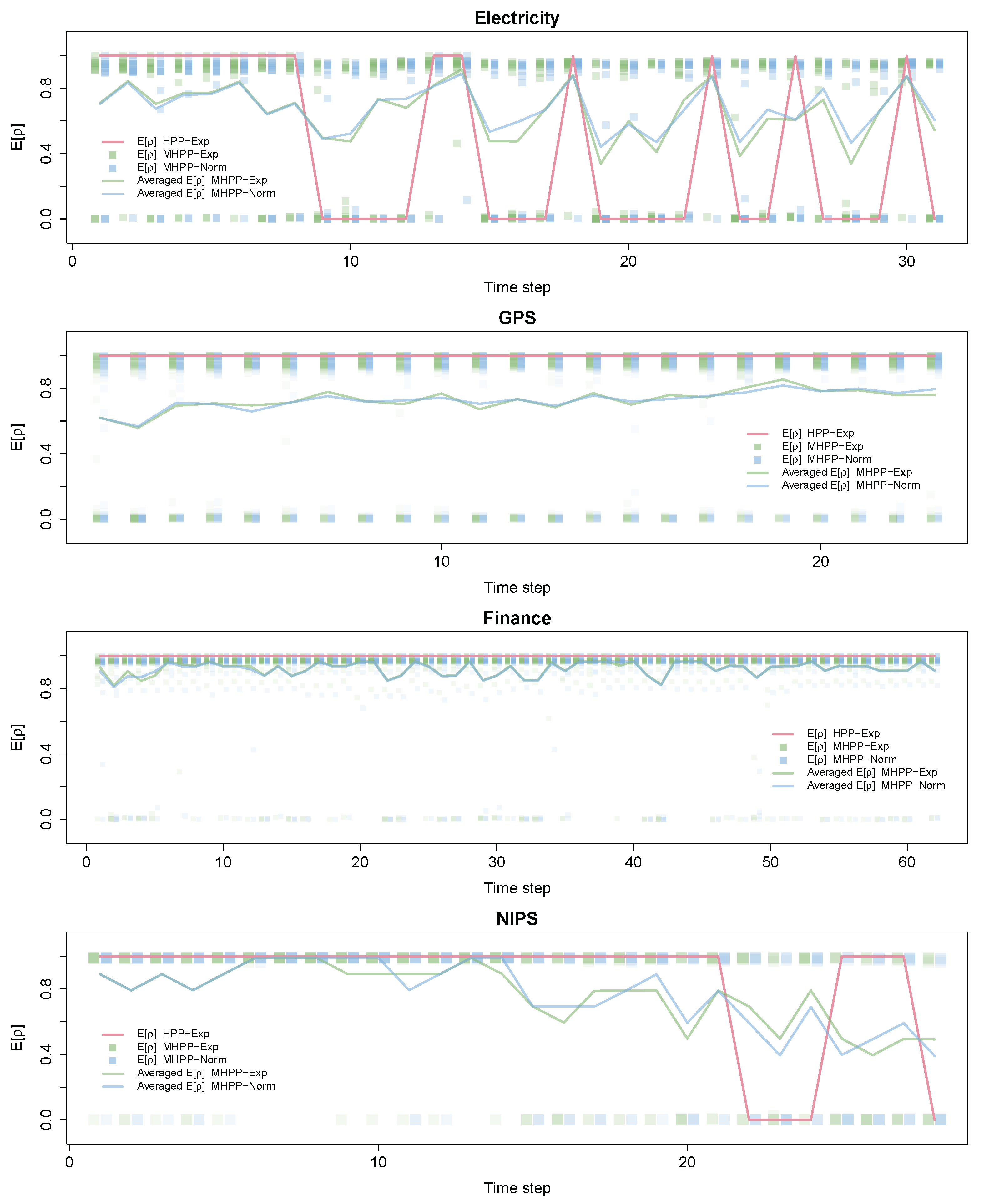
In this first part, we will highlight how the basic versions of SVB-HPP and SVB-MHPP outperform the rest of the approaches in most of the cases. Figure 7 shows for each method the difference between its TMLLt and that obtained by SVB (which is considered the baseline method). To improve readability, we only plot the results of the best performing method inside each group of methods. Figure 8 shows the development of over time for SVB-HPP-Exp, SVB-MHPP-Exp, and SVB-MHPP-Norm. For SVB-HPP-TExp, we only have one -parameter, and its value is given by the solid line. SVB-MHPP utilizes one for each variational parameter. (The numbers of variational parameters are 14, 78, 33, and 10 for the electricity, GPS, financial, and NIPS models, respectively.) In this case, we plot at each point in time to indicate the variability between the different estimates throughout the series. We also report the average of the values at every time step. Finally, we compute the aggregated test marginal log-likelihood measure for each method and report these values in Table 1.
For the electricity data set, we can see that the two proposed methods (SVB-HPP and SVB-MHPP) perform the best, as shown in Table 1. According to Figure 7 (electricity plot), all models are comparable during the first nine months, which is a period where our models detected no or very limited concept drift. However, after this period, both SVB-HPP and SVB-MHPP detected substantial drift and were able to adapt better than the other methods, which appeared unable to adjust to the complex concept drift structure in the latter part of the data. SVB-HPP and SVB-MHPP continued to behave at a similar level, mainly because when drift happened, it typically involved a high proportion of the parameters of the model (see the electricity plot in Figure 8).
For the GPS data set, we can observe how the SVB-MHPP perfoms quite well (see Table 1), particularly towards the end of the series (see the GPS plot in Figure 7). We can see in Figure 8 (GPS plot), that a significant proportion of the model parameters drifted (i.e., ) at all times, while another proportion of the parameters showed a quite stable behavior (-values above ). This complex pattern is not properly captured by SVB-HPP, which ends up assuming no concept drift. PVB with and does well here, but it strongly depends on the hyperparameters, as in fact any other hyperparameter combination yields poorer results (see Table 1).
The financial data set shows a different behavior. As can be seen in Figure 7 (Finance plot), during the first months, no major differences among the methods were found. However, after month 30, SVB-PP with is superior. Looking at the -values of SVB-MHPP in Figure 8 (Finance plot), we observe that there is remarkable concept drift in some of the parameters over the first few months. However, only a few parameters exhibit noteworthy drift after the first third of the sequence. Apparently, the simple SVB-PP approach has the upper hand when drift is constant and fairly limited, at least when the optimal forgetting factor has been identified.
In the case of the NIPS data set, we see again that HPP approaches capture drift in the data. As can be seen in Figure 7 (NIPS plot), SVB-HPP hardly detects any drift in the first 20 years and performs quite similarly to SVB (i.e., relative performance close to zero). However, in the last 10 years, SVB-HPP clearly outperforms SVB because it detects two strong drifts at years 23 and 29. Therefore, at these time steps, the whole LDA model is almost reestimated from scratch. In this case, SVB-MHPP is able to capture more fine-grained drifts in the data, as can been deduced from the -values of SVB-MHPP in Figure 8 (NIPS plot). Mainly, it detects changes in some topics while other topics remain constant over time. This allows SVB-MHPP to outperform SVB-HPP during some periods.
We have also observed that there are no major differences between SVB-MHPP-Exp and SVB-MHPP-Norm. Therefore, it seems that the inclusion of alternative priors does not have a big impact on the performance, at least if the variance parameter of the truncated normal is fixed automatically using an empirical Bayes approach. However, this is something that may require further investigations.
We conclude this section by highlighting that the performances of SVB-PP and PVB strongly depends on the hyperparameters of the model, cf. Table 1. As an example, consider SVB-PP and how its performance varies by changing the parameter. Similarly, PVB’s performance is sensitive both to (see in particular the results for the GPS data) and M (financial data). These hyperparameters are hard to fix, as their optimal values depend on data characteristics (see McInerney et al. [25] and Broderick et al. [27] for similar conclusions). We, therefore, believe that the fully Bayesian formulation is an important strong point of our approach.
7. Conclusions
In this paper, we have introduced a novel Bayesian approach for learning general latent variable models from nonstationary data streams. For this purpose, we introduce implicit transition models as a general method for transitioning the parameters of a latent variable model. We also show that previous approaches like exponential forgetting and power priors can be seen as specific cases of this general transition model. However, these approaches are only able to model slowly changing data streams. Our approach is able to handle both abrupt and gradual drifts in the data stream by explicitly modeling the rate of change of the data stream. For this purpose, we introduce a novel hierarchical prior which allows the model to adapt to the different drifts that one can encounter in a data stream. We then develop an efficient variational inference scheme that optimizes a novel lower bound of the likelihood function.
As future work, we aim to provide a sound approach to semantically characterize concept drift by inspecting the values provided by SVB-MHPP and to investigate the effects in variational approximation introduced by the use of the double lower bound approximation.
Author Contributions
Conceptualization, A.R.M., A.S., H.L., and T.D.N.; methodology, A.R.M., D.R.-L., A.S., H.L., and T.D.N.; software, A.R.M. and D.R.-L.; validation, A.R.M. and D.R.-L.; formal analysis, A.R.M., D.R.-L., A.S., H.L., and T.D.N.; investigation, A.R.M., D.R.-L., A.S., H.L., and T.D.N.; resources, A.S., H.L., and T.D.N.; data curation, A.R.M. and D.R.-L.; writing—original draft preparation, A.R.M.; writing—review and editing, A.R.M., D.R.-L., A.S., H.L., and T.D.N.; visualization, D.R.-L.; supervision, A.S., H.L., and T.D.N.; project administration, A.S., H.L., and T.D.N.; funding acquisition, A.S. All authors have read and agreed to the published version of the manuscript.
Funding
This research was funded by the Spanish Ministry of Economy and Competitiveness through projects TIN2015-74368-JIN and TIN2016-77902-C3-3-P and by ERDF funds and by the Ministry of Science and Innovation through the project PID2019-106758GB-C32. A.M., D.R.L., and A.S. thank the support from the Center for Development and Transfer of Mathematical Research to Industry CDTIME (University of Almería). D.R.L. thanks also the research group FQM-229 (Junta de Andalucía) and the “Campus de Excelencia Internacional del Mar” CEIMAR (University of Almería).
Conflicts of Interest
The authors declare no conflict of interest.
Appendix A. Proofs
Proof of Theorem 1.
(The proof follows [30].) To solve the constrain optimization problem, we define the following Lagrangian:
where the second component corresponds to the constrain imposing that q must be a valid density and that the last term is the constraint given in Equation (18).
Taking a derivative w.r.t. to and regrouping, we have
By setting the partial derivative to zero and regrouping, we have
If we exponentiate both arguments, we get the first Karush–Kuhn–Tucker condition:
The rest of Karush–Kuhn–Tucker conditions are
If , then we have that and satisfy Equations (A1)–(A4). If not, there must exist a satisfying that because we have that is smooth w.r.t. to ; when , we have that ; and when , we have that . Then, Equations (A1)–(A4) are also satisfied by this value. Finally, we can deduce Equation (19) by setting . □
Proof of Lemma 1.
Translate the recursive Bayesian updating approach of power priors into an equivalent two time slice model, where is given a prior distribution and is a Dirac delta function. The distribution in this model is equivalent to , which, in turn, is equivalent (up to proportionality) to . Note that the last term can alternatively be expressed as . □
Proof of Theorem 2.
It follows from Equations (30) and (31) that
According to Equation (21), if we ignore the base measure, we can write
Since is convex [49], we have
which combined with Equation (21) gives
Finally, by exploiting the mean field factorization of q and by using the exponential family form of and , we get the desired result. □
Proof of Corollary 1.
The first equality follows immediately from Equation (30) because the difference does not depend on and . The second equality holds because the difference between the natural gradients of and is equal to
According to Equation (19), the above difference is null if we make the parameter of the term equal to . □
Proof of Lemma 2.
Firstly, by ignoring the terms in (Equation (31)) that do not involve , we get
As we have assumed that the sufficient statistics function for and contains the identity function (), we have
where the subindex refers to those subindexes different from 1.
Using the standard equality of exponential family distributions, , we have
We can now find the natural gradient by premultiplying by the inverse of the Fisher information matrix, which for the exponential family corresponds to the inverse of the Hessian of the log-normalizer:
Then, by introducing inside the expectation, we get the difference in Kullbach–Leibler divergence . □
Appendix B. Probabilistic Models Used in the Experimental Evaluation
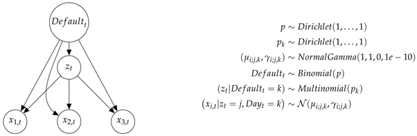
We provide a (simplified) graphical description of the probabilistic models used in the experiments. We also detail the distributional assumptions of the parameters, which are then used to define the variational approximation family.
Appendix B.1. Electricity Model

Appendix B.2. GPS Model

Appendix B.3. Financial Model
References
- Hastings, W.K. Monte Carlo sampling methods using Markov chains and their applications. Biometrika 1970, 57, 97–109. [Google Scholar] [CrossRef]
- Gelfand, A.E.; Smith, A.F. Sampling-based approaches to calculating marginal densities. J. Am. Stat. Assoc. 1990, 85, 398–409. [Google Scholar] [CrossRef]
- Gama, J.; Žliobaitė, I.; Bifet, A.; Pechenizkiy, M.; Bouchachia, A. A survey on concept drift adaptation. ACM Comput. Surv. 2014, 46, 1–37. [Google Scholar] [CrossRef]
- Blei, D.M.; Ng, A.Y.; Jordan, M.I. Latent Dirichlet allocation. J. Mach. Learn. Res. 2003, 3, 993–1022. [Google Scholar]
- Borchani, H.; Martínez, A.M.; Masegosa, A.R.; Langseth, H.; Nielsen, T.D.; Salmerón, A.; Fernández, A.; Madsen, A.L.; Sáez, R. Modeling concept drift: A probabilistic graphical model based approach. In International Symposium on Intelligent Data Analysis; Springer: Cham, Switzerland, 2015; pp. 72–83. [Google Scholar]
- Rabiner, L.R.; Juang, B.H. An introduction to hidden Markov models. IEEE ASSP Mag. 1986, 3, 4–16. [Google Scholar] [CrossRef]
- Bishop, C.M. Latent variable models. In Learning in Graphical Models; Springer: Dordrecht, The Netherlands, 1998; pp. 371–403. [Google Scholar]
- Blei, D.M. Build, compute, critique, repeat: Data analysis with latent variable models. Annu. Rev. Stat. Its Appl. 2014, 1, 203–232. [Google Scholar] [CrossRef] [Green Version]
- Bishop, C.M. Pattern Recognition and Machine Learning; Springer: New York, NY, USA, 2006. [Google Scholar]
- Tipping, M.E.; Bishop, C.M. Probabilistic principal component analysis. J. R. Stat. Soc. Ser. B Stat. Methodol. 1999, 61, 611–622. [Google Scholar] [CrossRef]
- Koller, D.; Friedman, N. Probabilistic Graphical Models: Principles and Techniques; MIT Press: Cambridge, MA, USA, 2009. [Google Scholar]
- Murphy, K.P. Machine Learning: A Probabilistic Perspective; MIT Press: Cambridge, MA, USA, 2012. [Google Scholar]
- Blei, D.M.; Kucukelbir, A.; McAuliffe, J.D. Variational inference: A review for statisticians. J. Am. Stat. Assoc. 2017, 112, 859–877. [Google Scholar] [CrossRef] [Green Version]
- Hamilton, J.D. Time Series Analysis; Princeton University Press: Princeton, NJ, USA, 1994; Volume 2. [Google Scholar]
- Triantafyllopoulos, K. Inference of dynamic generalized linear models: On-line computation and appraisal. Int. Stat. Rev. 2009, 77, 430–450. [Google Scholar] [CrossRef]
- Chen, X.; Irie, K.; Banks, D.; Haslinger, R.; Thomas, J.; West, M. Scalable Bayesian Modeling, Monitoring, and Analysis of Dynamic Network Flow Data. J. Am. Stat. Assoc. 2018, 113, 519–533. [Google Scholar] [CrossRef] [Green Version]
- Aminikhanghahi, S.; Cook, D.J. A survey of methods for time series change point detection. Knowl. Inf. Syst. 2017, 51, 339–367. [Google Scholar] [CrossRef] [PubMed] [Green Version]
- Adams, R.P.; MacKay, D.J. Bayesian online changepoint detection. arXiv 2007, arXiv:0710.3742. [Google Scholar]
- Gaber, M.M.; Zaslavsky, A.; Krishnaswamy, S. Mining data streams: A review. ACM Sigmod Rec. 2005, 34, 18–26. [Google Scholar] [CrossRef]
- Aggarwal, C.C. Data Streams: Models and Algorithms; Springer: New York, NY, USA, 2007; Volume 31. [Google Scholar]
- Gama, J.; Rodrigues, P.P. An overview on mining data streams. In Foundations of Computational, Intelligence; Springer: Berlin/Heidelberg, Germany, 2009; Volume 6, pp. 29–45. [Google Scholar]
- Aggarwal, C.C. Managing and Mining Sensor Data; Springer: New York, NY, USA, 2013. [Google Scholar]
- Papadimitriou, S.; Sun, J.; Faloutsos, C. Streaming pattern discovery in multiple time-series. In Proceedings of the 31st International Conference on Very Large Data Bases, VLDB Endowment, Trondheim, Norway, 30 August–2 September 2005; pp. 697–708. [Google Scholar]
- Honkela, A.; Valpola, H. On-line variational Bayesian learning. In Proceedings of the 4th International Symposium on Independent Component Analysis and Blind Signal Separation, Nara, Japan, 1–4 April 2003; pp. 803–808. [Google Scholar]
- McInerney, J.; Ranganath, R.; Blei, D. The population posterior and Bayesian modeling on streams. In Advances in Neural Information Processing Systems 28; Curran Associates, Inc.: Montreal, QC, Canada, 2015; pp. 1153–1161. [Google Scholar]
- Hoffman, M.D.; Blei, D.M.; Wang, C.; Paisley, J. Stochastic variational inference. J. Mach. Learn. Res. 2013, 14, 1303–1347. [Google Scholar]
- Broderick, T.; Boy, N.; Wibisono, A.; Wilson, A.C.; Jordan, M.I. Streaming variational Bayes. In Advances in Neural Information Processing Systems 26; Curran Associates, Inc.: Lake Tahoe, NV, USA, 2013; pp. 1727–1735. [Google Scholar]
- Ibrahim, J.G.; Chen, M.H. Power prior distributions for regression models. Stat. Sci. 2000, 15, 46–60. [Google Scholar]
- Ibrahim, J.G.; Chen, M.H.; Sinha, D. On optimality properties of the power prior. J. Am. Stat. Assoc. 2003, 98, 204–213. [Google Scholar] [CrossRef]
- Ozkan, E.; Smidl, V.; Saha, S.; Lundquist, C.; Gustafsson, F. Marginalized adaptive particle filtering for nonlinear models with unknown time-varying noise parameters. Automatica 2013, 49, 1566–1575. [Google Scholar] [CrossRef]
- Kárnỳ, M. Approximate Bayesian recursive estimation. Inf. Sci. 2014, 285, 100–111. [Google Scholar] [CrossRef]
- Shi, T.; Zhu, J. Online Bayesian passive-aggressive learning. J. Mach. Learn. Res. 2017, 18, 1–39. [Google Scholar]
- Williamson, S.; Orbanz, P.; Ghahramani, Z. Dependent Indian buffet processes. In Proceedings of the Thirteenth International Conference on Artificial Intelligence and Statistics, Sardinia, Italy, 13–15 May 2010; pp. 924–931. [Google Scholar]
- Blei, D.M.; Lafferty, J.D. Dynamic topic models. In Proceedings of the 23rd International Conference on Machine Learning, Pittsburgh, PA, USA, 25–29 June 2006; pp. 113–120. [Google Scholar]
- Williamson, S.; Wang, C.; Heller, K.; Blei, D. The IBP compound Dirichlet process and its application to focused topic modeling. In Proceedings of the 27th International Conference on Machine Learning, Haifa, Israel, 21–24 June 2010. [Google Scholar]
- Perrone, V.; Jenkins, P.A.; Spano, D.; Teh, Y.W. Poisson random fields for dynamic feature models. J. Mach. Learn. Res. 2017, 18, 1–45. [Google Scholar]
- Brown, L.D. Fundamentals of Statistical Exponential Families: With Applications in Statistical Decision Theory; Institute of Mathematical Statistics: Hayward, CA, USA, 1986. [Google Scholar]
- Bernardo, J.M.; Smith, A.F. Bayesian Theory; John Wiley & Sons: New York, NY, USA, 2009; Volume 405. [Google Scholar]
- Heckerman, D.; Geiger, D.; Chickering, D.M. Learning Bayesian networks: The combination of knowledge and statistical data. Mach. Learn. 1995, 20, 197–243. [Google Scholar] [CrossRef] [Green Version]
- Masegosa, A.R.; Martinez, A.M.; Langseth, H.; Nielsen, T.D.; Salmerón, A.; Ramos-López, D.; Madsen, A.L. Scaling up Bayesian variational inference using distributed computing clusters. Int. J. Approx. Reason. 2017, 88, 435–451. [Google Scholar] [CrossRef]
- Winn, J.M.; Bishop, C.M. Variational message passing. J. Mach. Learn. Res. 2005, 6, 661–694. [Google Scholar]
- Olesen, K.G.; Lauritzen, S.L.; Jensen, F.V. aHUGIN: A system creating adaptive causal probabilistic networks. In Proceedings of the Eighth International Conference on Uncertainty in Artificial Intelligence, Stanford, CA, USA, 17–19 July 1992; Morgan Kaufmann Publishers Inc.: San Francisco, CA, USA, 1992; pp. 223–229. [Google Scholar]
- Lauritzen, S.L. Propagation of probabilities, means, and variances in mixed graphical association models. J. Am. Stat. Assoc. 1992, 87, 1098–1108. [Google Scholar] [CrossRef]
- Sato, M.A. Online model selection based on the variational Bayes. Neural Comput. 2001, 13, 1649–1681. [Google Scholar] [CrossRef]
- Harries, M. Splice-2 Comparative Evaluation: Electricity Pricing; NSW-CSE-TR-9905; School of Computer Siene and Engineering, The University of New South Wales: Sydney, Australia, 1999. [Google Scholar]
- Zheng, Y.; Li, Q.; Chen, Y.; Xie, X.; Ma, W.Y. Understanding mobility based on GPS data. In Proceedings of the 10th International Conference on Ubiquitous Computing, UbiComp ’08, Seoul, Korea, 21–24 September 2008; ACM: New York, NY, USA, 2008; pp. 312–321. [Google Scholar] [CrossRef]
- Zheng, Y.; Zhang, L.; Xie, X.; Ma, W.Y. Mining interesting locations and travel sequences from GPS trajectories. In Proceedings of the 18th International Conference on World Wide Web, WWW ’09, Madrid, Spain, 20–24 April 2009; ACM: New York, NY, USA, 2009; pp. 791–800. [Google Scholar] [CrossRef] [Green Version]
- Zheng, Y.; Xie, X.; Ma, W.Y. GeoLife: A collaborative social networking service among user, location and trajectory. IEEE Data Eng. Bull. 2010, 33, 32–39. [Google Scholar]
- Wainwright, M.J.; Jordan, M.I. Graphical models, exponential families, and variational inference. Found. Trends® Mach. Learn. 2008, 1, 1–305. [Google Scholar] [CrossRef] [Green Version]
Figure 1.
The left figure (a) displays a graphical representation of the probabilistic model examined in this paper (see Section 3.1). The right figure (b) includes a temporal evolution model for as described in Section 5. The graphical notation corresponds to probabilistic graphical models with plateau notation [11]. Under this notation, a random variable is represented by a node, and it is conditionally dependent on those random variables with a node pointing to it. The nodes within the box denote random variables that are replicated for every data sample.
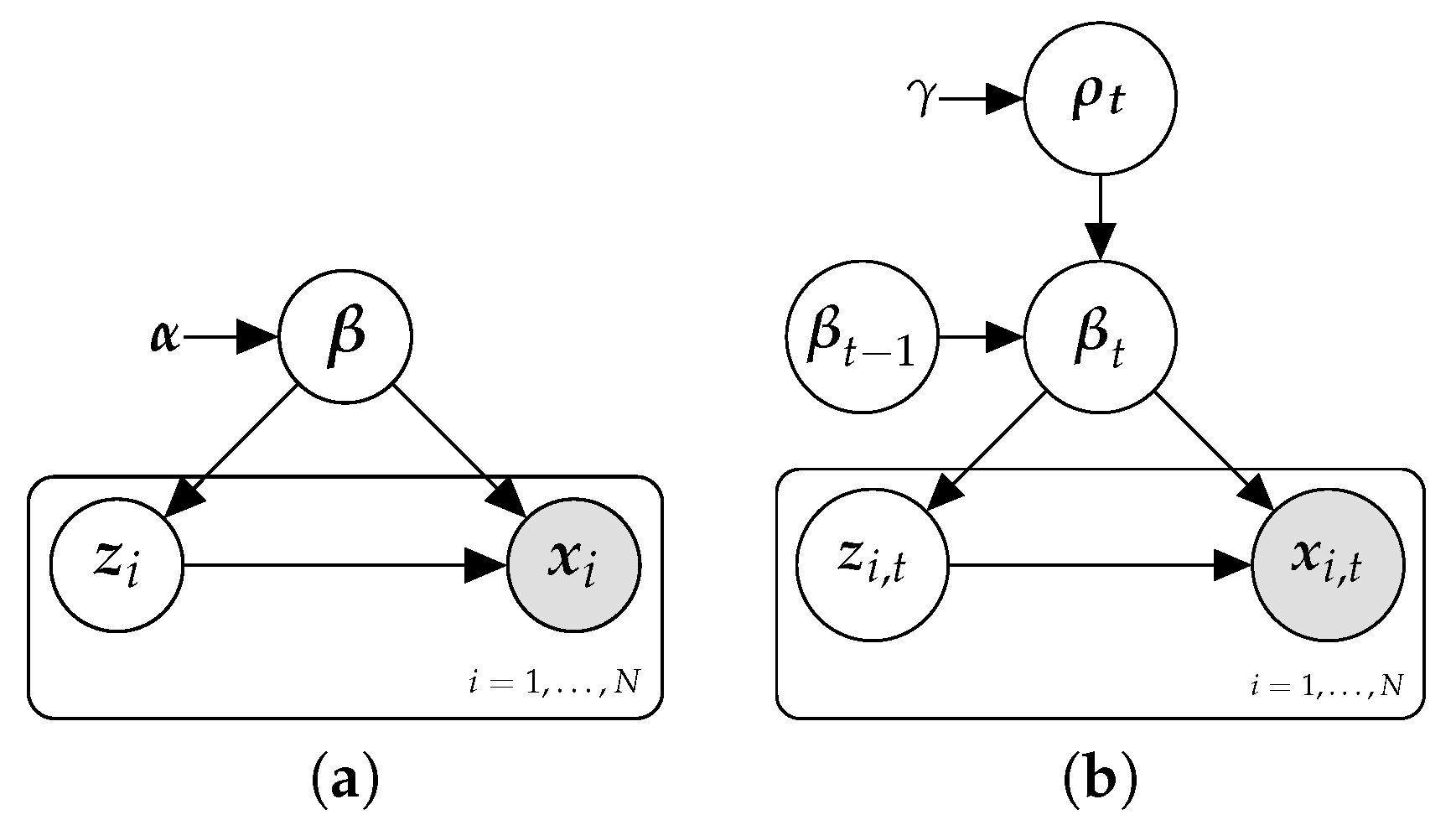
Figure 2.
Density functions of the truncated exponential and the truncated normal distributions, respectively, for different values of their parameters.
Figure 2.
Density functions of the truncated exponential and the truncated normal distributions, respectively, for different values of their parameters.
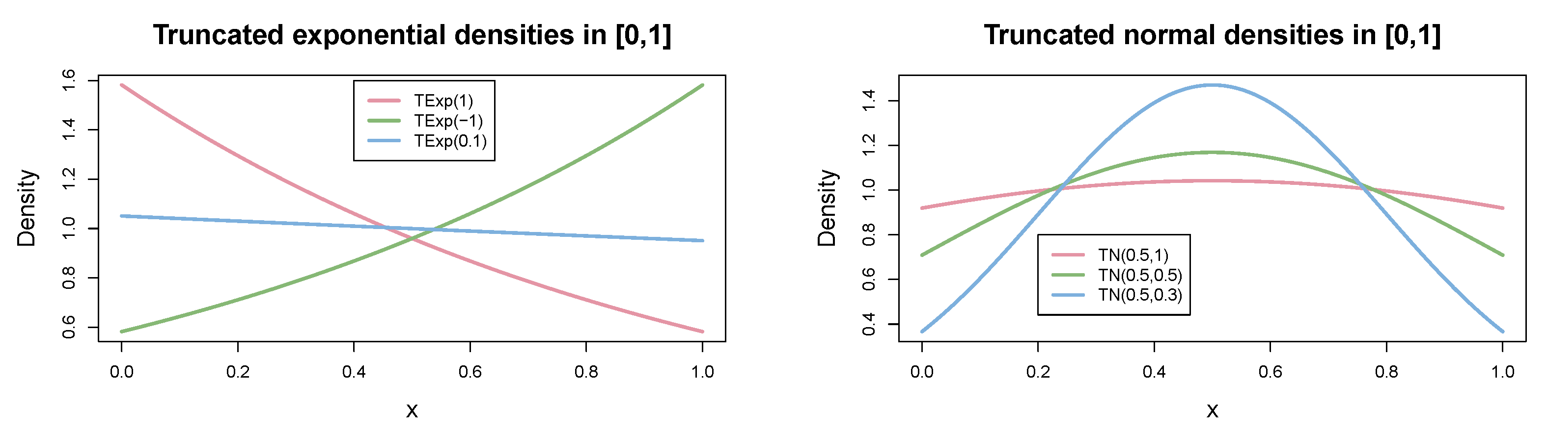
Figure 3.
The relationship between and according to Equation (28) (left) and Equation (29) (right): see Section 5.3 for details.
Figure 3.
The relationship between and according to Equation (28) (left) and Equation (29) (right): see Section 5.3 for details.
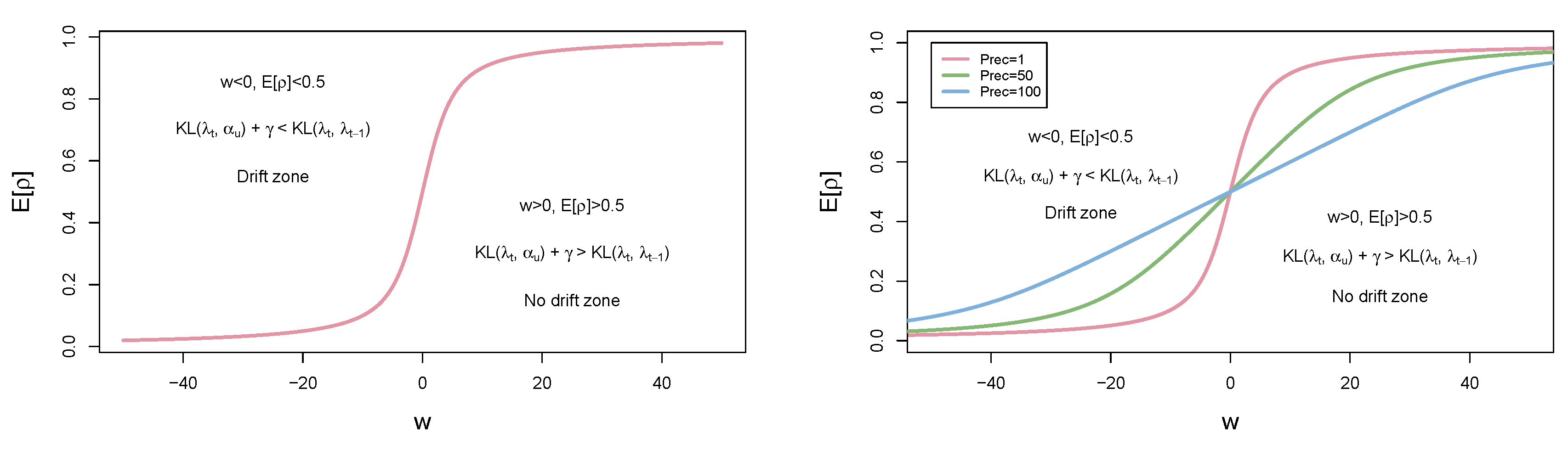
Figure 4.
Example with Gaussian posterior distribution are shown. Two possible situations: no concept drift (left) when is closer to than to (in terms of KL divergence); otherwise (right), there is concept drift. See Section 5.3 for details.
Figure 4.
Example with Gaussian posterior distribution are shown. Two possible situations: no concept drift (left) when is closer to than to (in terms of KL divergence); otherwise (right), there is concept drift. See Section 5.3 for details.

Figure 5.
in the beta-binomial model artificial data set: note that PVB-1000-0.1 overlaps with SVB-PP-0.9 and PVB-1000-0.01 overlaps with SVB-PP-0.99. The exact value is denoted with red circles.
Figure 5.
in the beta-binomial model artificial data set: note that PVB-1000-0.1 overlaps with SVB-PP-0.9 and PVB-1000-0.01 overlaps with SVB-PP-0.99. The exact value is denoted with red circles.

Figure 6.
The results for the beta-binomial model artificial data set. Left panel: The equivalent sample size of the posterior, , for the different methods; the values for SVB-HPP are shown on the right y-axis. Right panel: The expected values of , , for batches of size 100 and 1000, respectively.
Figure 6.
The results for the beta-binomial model artificial data set. Left panel: The equivalent sample size of the posterior, , for the different methods; the values for SVB-HPP are shown on the right y-axis. Right panel: The expected values of , , for batches of size 100 and 1000, respectively.
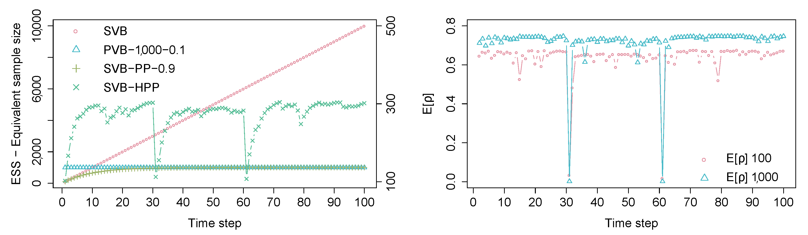
Figure 7.
Results of the TMLLt improvement over SVB for the competing methods for the four real data sets.
Figure 7.
Results of the TMLLt improvement over SVB for the competing methods for the four real data sets.
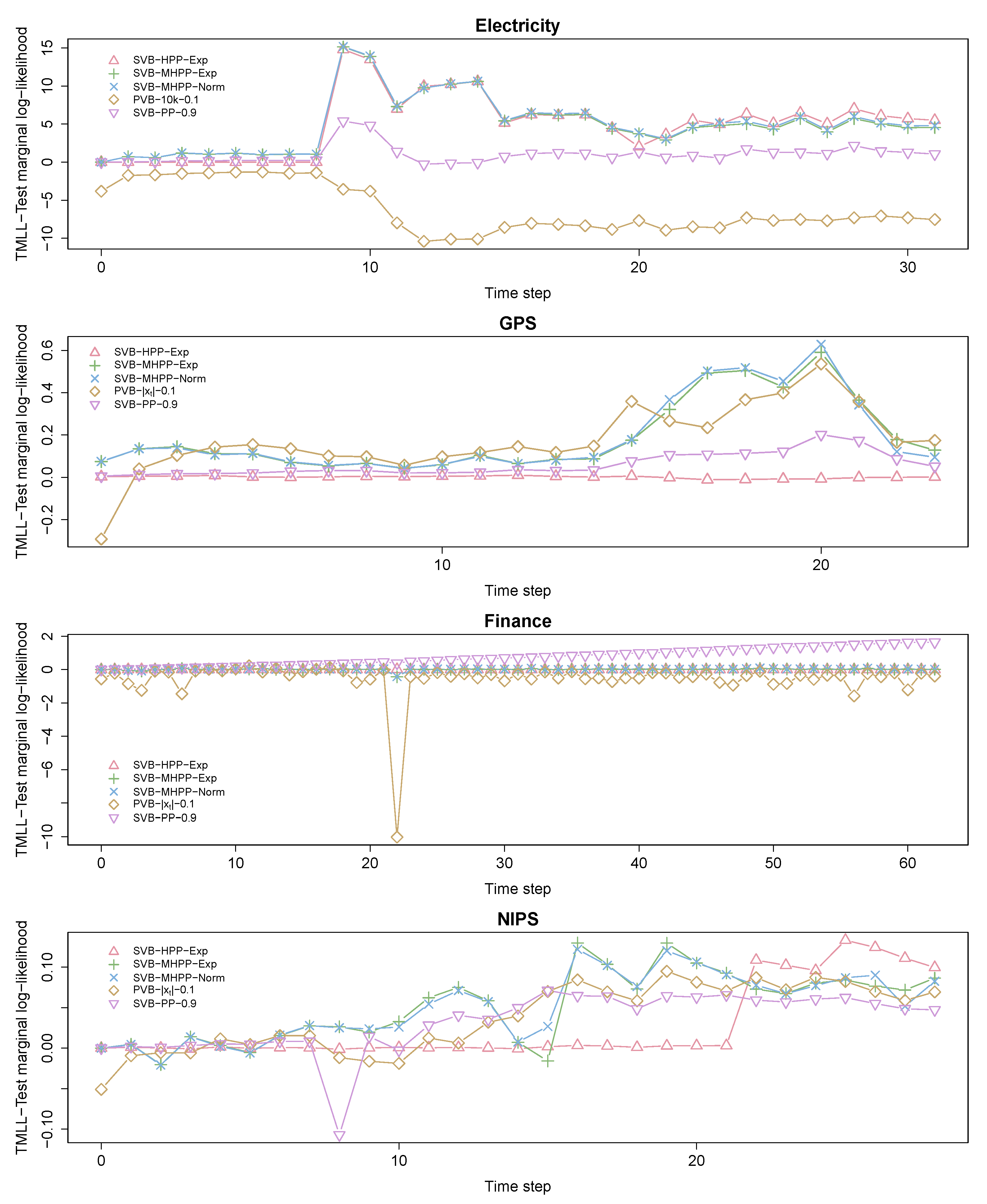
Figure 8.
Evolution of for SVB-HPP and SVB-multiple hierarchical power prior (MHPP).

Table 1.
Aggregated test marginal log-likelihood: maximum values for each data set are boldfaced.
| Data Set | SVB | PVB | SVB-PP | SVB-HPP | SVB-MHPP | |||||
|---|---|---|---|---|---|---|---|---|---|---|
| (1) | (2) | (3) | (4) | Exp | Exp | Norm | ||||
| Electricity | −44.91 | −51.01 | −52.19 | −51.11 | −61.70 | −43.92 | −44.80 | −40.05 | −40.02 | −39.91 |
| GPS | −1.98 | −2.10 | −2.77 | −1.97 | −4.49 | −1.94 | −1.97 | −1.97 | −1.86 | −1.86 |
| Finance | −19.84 | −22.29 | −22.57 | −20.40 | −20.73 | −19.05 | −19.78 | −19.83 | −19.83 | −19.82 |
| NIPS | −4.07 | −4.04 * | −4.21 * | −4.01 | −4.12 | −4.02 | −4.06 | −4.01 | −4.00 | −4.00 |
Population variational Bayes (PVB) parameters: (1) ; (2) ; (3) ; and (4) . (*) For NIPS, was used in (1) and (2).
Publisher’s Note: MDPI stays neutral with regard to jurisdictional claims in published maps and institutional affiliations. |
© 2020 by the authors. Licensee MDPI, Basel, Switzerland. This article is an open access article distributed under the terms and conditions of the Creative Commons Attribution (CC BY) license (http://creativecommons.org/licenses/by/4.0/).
Share and Cite
MDPI and ACS Style
Masegosa, A.R.; Ramos-López, D.; Salmerón, A.; Langseth, H.; Nielsen, T.D. Variational Inference over Nonstationary Data Streams for Exponential Family Models. Mathematics 2020, 8, 1942. https://doi.org/10.3390/math8111942
AMA Style
Masegosa AR, Ramos-López D, Salmerón A, Langseth H, Nielsen TD. Variational Inference over Nonstationary Data Streams for Exponential Family Models. Mathematics. 2020; 8(11):1942. https://doi.org/10.3390/math8111942
Chicago/Turabian StyleMasegosa, Andrés R., Darío Ramos-López, Antonio Salmerón, Helge Langseth, and Thomas D. Nielsen. 2020. "Variational Inference over Nonstationary Data Streams for Exponential Family Models" Mathematics 8, no. 11: 1942. https://doi.org/10.3390/math8111942
Note that from the first issue of 2016, this journal uses article numbers instead of page numbers. See further details here.