Abstract
The snap-off is an instability phenomenon that takes place during the immiscible two-phase flow in porous media due to competing forces acting on the fluid phases and at the interface between them. Different theoretical approaches have been proposed for the development of mathematical models that describe the dynamics of a fluid/fluid interface in order to analyze the snap-off mechanism. The models studied here are based on the “small-slope” approach and were derived from the mass conservation and other governing equations of two-phase flow at pore scale in circular capillaries for pure and complex interfaces. The models consist of evolution equations; highly nonlinear partial differential equations of fourth order in space and first order in time. Although the structure of the models for each type of interface is similar, different numerical techniques have been employed to solve them. Here, we propose a unifying numerical framework to solve the group of such models. Such a framework is based on the Fourier pseudo-spectral differentiation method which uses the Fast Fourier Transform (FFT) and the inverse FFT (IFFT) algorithms. We compared the solutions obtained with this method to the results reported in the literature in order to validate our framework. In general, acceptable agreements were obtained in the dynamics of the snap-off.
1. Introduction
When a fluid displaces another in a porous media, different displacement mechanisms may occur depending on the local flow conditions. The displacement may occur in a piston-like regime, at which one phase is fully pushed by the other, or the displacing liquid may leave a thin film at the wall forming an interface between the two fluids. If the capillary forces are strong enough, the thin film attached to the wall may form a liquid collar and could break up the displacing phase into separate ganglia due to surface tension. This instability phenomenon is known as snap-off (Figure 1). The occurrence of snap-off is determined by competing forces acting on the fluid phases and at the interface between them: the capillary pressure difference that drives the wetting phase towards the constriction, the shear stress at the interface that resists the capillary driven flow and the squeezing process of the non-wetting phase [1].
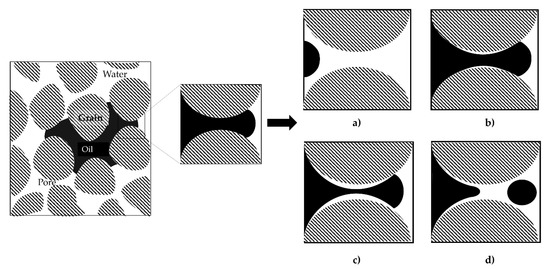
Figure 1.
Snap-off phenomenon illustration in a water wet porous media which contains residual oil ganglia (in black). Snap-off occurs when: (a) the front of the non-wetting phase flows near the pore throat; (b) Then the wetting phase is displaced by the non-wetting one, leaving a thin film at the wall; (c) A liquid collar of the wetting phase grows due to the capillary pressure difference at the crest and the capillary throat; (d) The collar breaks up the displacing phase due to the surface tension and a separate ganglion is formed.
The snap-off phenomenon is important to many industrial and technological areas such as biofluid dynamics, CO2 geological sequestration, oil recovery, microfluidic devices and chemical engineering. This phenomenon has been studied both experimentally and theoretically for viscous (drops) and inviscid (bubbles) fluids. This paper is focused on the theoretical approach. According to Deng et al., [2] the theoretical snap-off studies typically have two goals: development of models which describe the evolution of the interface between the fluids until snap-off is achieved and the definition of a snap-off criterion. The interface evolution models are used to test snap-off criteria and quantify the snap-off time.
Different approaches have been proposed for the development of mathematical models that describe the dynamics of a fluid/fluid interface [3,4,5,6,7,8]. Here we focused on the models that describe the drop and bubble snap-off in circular capillaries by means of an evolution equation derived from the conservation of mass equation and the small-slope approach [9,10]. This approach consists in the improvement of the approximation of the Young–Laplace equation; that is, in the balance of the pressure forces that have their expression in the curvature of the interface. The small slope approach assumes small capillary and Reynolds numbers, which allow the flow in the capillary to be approximated as Poiseuillean flow. Furthermore, it is assumed that the radius of the pore wall varies to a small extent relative to the axial distance, so lubrication approximation applies [11]. The models derived under this approach have been solved with diverse numerical techniques.
Hammond [12] performs a nonlinear analysis based on lubrication theory in order to examine the core-annular flow instability in straight and circular capillaries. The analysis results in a nonlinear thin-film evolution equation. To solve this model, he used the Method of Lines (MOL), which consists of replacing the spatial derivatives with finite differences that generate a system of coupled ordinary differential equations (ODE) for the time evolution of the gas–liquid interface; the ODE system is solved with the Gear’s method.
Gauglitz and Radke [9,10] extended the Hammond’s evolution equation by making higher order corrections in the thin-film analysis; this resulted in the small-slope approximation. The small-slope equations have a more complex mathematical form compared to the thin-film ones; this is due to a better approximation of the Young–Laplace equation. To analyze the film breakup in both straight and constricted cylindrical capillaries, they implement the Galerkin Finite Element (GFE) method to solve their model. They used Hermite cubic basis functions, and the time derivatives are discretized with the Crank–Nicholson procedure. The resulting system of algebraic equations is solved by iterations with the Newton–Raphson method.
Zhang et al. [13] solved the Gauglitz and Radke (GR) model for straight capillaries by using the MATLAB “pdepe” solver. However, they had to do a reduction of order transformation in order to adapt the problem to the algorithm requirements. The “pdepe” algorithm solves the initial boundary value problems for parabolic-elliptic partial differential equations (PDE) in 1-D using the MOL, where the spatial variable is discretized according with Skeel and Berzins [14] with Petrov–Galerkin’s approach. This results in a system of ordinary differential equations that are solved using a variable-step, variable-order algorithm based on the numerical differentiation formulas of orders 1 to 5 [15].
Recently, Hoyer et al. [16] extended the GR model including elastic interfacial stress to analyze the behavior of the breakup process in complex interfaces. The interfacial elasticity makes the surface stress anisotropic, which has a direct effect on the pressure along the liquid film. For inelastic cases, the Hoyer and coworkers (HAC) model becomes a more accurate formulation since the GR model linearizes the logarithmic terms and discards the film thickness terms of an order greater than three (thin-film assumption). Such discrimination can generate important differences, for example, in snap-off time (close to a factor of 2) when the models are tested at high capillary numbers. To solve their model, suitable for the case of dispersed drop viscosity much lower than the continuous phase, they used an explicit Euler first order finite difference method, also known as Forward Euler (FE).
Additionally, Beresnev and Deng [17] developed an evolution equation that describes the temporal evolution in a fluid–fluid interface for arbitrary viscosities in the presence of base flow. The Beresnev and Deng (BD) model is solved with the MOL framework implemented in Mathematica [18]. Furthermore, they validate their model with Computational Fluid Dynamics (CFD) experiments in two commercial models: FLUENT and COMSOL. To discretize the governing equations of flow, FLUENT uses the finite volume element method, while COMSOL use finite elements; for tracking the interface position the first uses the volume-of-fluid method and the second one the level-set method. Note that the computing time in the case of BD model is in the order of minutes, while CFD experiments took at least 1 day per scenario.
It is from this general review, that we can appreciate that there is great diversity in the schemes traditionally used to solve the models of the different interfaces reported (gas–liquid elastic, gas–liquid and liquid–liquid). This situation may be considered as restrictive when it is necessary to assess the effects of different fluids in a two-phase flow system under instability conditions. We, therefore, propose a unifying pseudo-spectral differentiation framework in which the most important reported models are solved. To validate our framework, we compare the solutions obtained using this method with those reported by our reference authors utilizing other numeric techniques.
This article is divided into four parts. Section 2, called Materials and Methods, first presents the geometry of the problem. Later, some considerations to derive the evolution equations from the governing equations of flow at pore-scale are briefly presented. Since the formulation of each model has its own particularities that depend on the fluid/fluid system, the main assumptions considered to represent the rheological nature of each type of interface are also mentioned. Then the models are presented in their dimensionless form, as well as the corresponding boundary and initial conditions. The last part of this section is dedicated to present Fourier pseudo-spectral differentiation method. Following that, Section 3 includes the results of the evaluation of the models using the framework proposed here, as well as a comparison with those reported in the literature. Section 4 contains the conclusions of our research.
2. Materials and Methods
2.1. Geometry of the Problem
The porous structure of a reservoir presents complex geometric shapes; among these, the presence of constrictions in the capillary channels called pore throats is found. Constricted pore geometry is typical of natural core-annular flows and can determinate the fluid breakup occurrence. During core-annular flow, the pores have a preference to be wetted by one of the phases, either water or oil, whereby one layer of the wetting phase will be present between the pore-wall and the non-wetting phase. This fluids configuration and geometry are schematized in Figure 2.
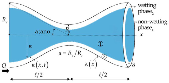
Figure 2.
Geometric diagram that shows circular constricted capillaries and the configuration of the liquid phases. The main geometric elements are the radius of the capillary ; the throat radius , and the length of the capillary . The configuration of the phases consists of a core-annular flow, in which the external phase (with subscript 2), with constant thickness and viscosity , wet the wall of a pore described by ; and the internal phase, with viscosity , is surrounded by the external phase, with which it shares the interface The volumetric flow , moves from left to right.
This basic geometry of the porous medium, consisting of a circular capillary with one or more constrictions, has been used to study the mechanism of drop breakup during the immiscible two-phase flow at pore-scale. Although any smooth function can be used to represent this particular geometry, a sinusoidal function is typically used [17]:
where is the radial coordinate of the capillary wall, refers to the axial coordinate, is the ratio between the throat () and capillary () radii and is a geometric parameter which represents the ratio between the capillary radius () and half of the capillary length , .
2.2. Governing Equations
The governing equations for a two-phase flow at pore scale are the simplified Navier–Stokes equations (momentum equation) using the lubrication approximation for incompressible and laminar flow in cylindrical coordinates, the conservation of mass, continuity and the Young–Laplace law derived under small-slope approach [17]:
where is the pressure, subscripts 1 and 2 denote, respectively, the non-wetting and wetting phase, is the dynamic viscosity, the radial coordinate, is the axial velocity, the temporal variable, the total volumetric flow rate in the capillary, is the capillary pressure, the radius of interface and the surface tension.
The drop breakup problem needs to determine the interface position change over time , thus the equations that govern the two-phase flow at pore scale are combined to establish an evolution equation that describes the interface dynamics. The evolution equation is derived from the mathematical expression of the conservation of mass (Equation (3)), which relates the change rate of the volume of some of the phases with the volumetric flow differential, which can be written in the form:
In order to close the evolution equation, the volume flux of the non-wetting phase is required to be explicitly expressed through the interface position . The evolution equation derived from this process will depend on the nature of the fluid phases, though its own particularities are further detailed in Section 2.3.1.
2.3. Drop and Bubble Snap-Off Models
In this section, we present the reported model’s equations that describe the snap-off dynamics in circular capillaries for elastic gas–liquid, gas–liquid and liquid–liquid interfaces. Even if original works can be consulted for further details of mathematical procedure for models derivation [9,10,16,17], it is important to specify the physical assumptions taken for such derivation.
2.3.1. General Considerations for the Derivation of Models
In general terms, the evolution equations that describe the temporal evolution of the interface are basically obtained by solving the simplified incompressible Navier–Stokes equations (momentum equation) for cylindrical core-annular geometry (Equation (2)); with which the velocity profiles of the wetting and non-wetting phases are obtained. The velocity profiles are integrated to obtain the volume flow rates. The resultant formulations are combined with the continuity and Young–Laplace equations (Equations (4) and (5)) to obtain an explicit expression of the volume flux through the interface position , which is finally substituted in the conservation equation (Equation (6)).
Depending on the core phase nature, two approaches can be distinguished: (1) those that consider an inviscid core fluid and constant zero pressure (GR and HAC models) (2) those in which a viscous core liquid is studied (BD model). For both cases, non-slip (solid wall) at the surface of the capillary () and balance of forces at the interface are postulated as boundary conditions. Additionally, this model assumes that the interface is infinitesimally thin and in a state of physic-chemical and mechanical equilibrium; therefore, no transport phenomena occurs.
In the first approach, since the viscosity of the non-wetting phase is null (), shear stress of the core is neglected ; consequently . In Hoyer and coworkers formulation [16] for elastic interfaces, surfaces stress () in axial () and transversal () directions are included as function of the surface tension , the dilational interfacial elasticity and the corresponding surface strains and (defined by geometric relationships). Note that for inelastic cases , the surface stress becomes . At the interface the liquid film shear stress is balanced by the net surfaces stress in axial direction, then: . Furthermore, a constant zero pressure is assumed for inviscid core (), thus explicit expressions based on the interface curvature for the capillary pressure can be used: for inelastic case the Young–Laplace equation becomes ; while for an elastic interface the expression is .
For fluid arbitrary viscosities (), the velocity profile of the core is equal to that of the annular film at the interface (); additionally no variation of the radial velocity derivative on the axes is postulated . In this case the assumption of constant zero pressure in the core is no longer valid, and Laplace’s law would only provide a relative pressure difference between the two fluids, it is expressed as: .
The nondimensionalizing is performed according with:
where * denotes dimensionless variables and is the film thickness. For the viscous core case, the dimensionless equations use the viscosity of the non-wetting phase instead of the wetting phase , and the dimensionless time is
2.3.2. Inviscid Core Fluid Models
Hoyer and coworkers (HAC) model for an elastic behavior of a gas–liquid interface, encapsulated in parameter, is denoted by the following formulation [16]:
if , i.e., for inelastic interface, it then results in an extension of the GR model [16]:
The Gauglitz and Radke model (GR) for the gas-liquid interface is [10]:
here the second factor on the derivative corresponds to an approximation of the equivalent term in the HAC model. For straight capillaries, i.e., , the GR model results in:
2.3.3. Viscous Core Fluid Models
The Beresnev and Deng model (BD) for liquid–liquid interfaces is [17]:
2.4. Initial and Boundary Conditions
The models presented here consist of fourth order partial differential equation in space and first order in time. A uniform film thickness is assumed as an initial condition in all cases. For the HAC and GR models, fourth boundary conditions are required, while in BD model periodic boundary conditions are postulated.
2.4.1. Initial Conditions
The initial conditions are related to the residual film of liquid wetting the adjacent wall of the capillary that is formed when it is displaced by the non-wetting fluid. When the invading phase is gas (HAC and GR models), Bretherton’s theory [19] predicts the dimensionless thickness of the wetting film as a power law of the capillary number
Beresnev et al. [20] developed a hydrodynamic theory and performed microfluidic experiments for two liquids core-annular flow (BD model). They concluded that Bretherton’s equation does not apply to liquid–liquid displacement. Deng et al. [21] used these experimental measurements and fitted them to propose an empirical equation in order to predict the film thickness under these flow conditions:
2.4.2. Boundary Conditions
For HAC and GR models, the two first boundary conditions are related with the assumption that the bubble is centered at the neck of the throat, consequently the problem is considered symmetric. Thus the interface profile should be perpendicular to the plane and no flow at the pore neck is imposed; i.e., the first and third derivatives are equal to zero at :
The rest of the boundary conditions are imposed away of the constriction, at a distance , where no movement in the interface is detected, thus:
Periodic boundary conditions for the BD model are imposed, that is, the interface radius is equal at the boundaries for all simulation time:
It should be noted that with this boundary conditions gas-liquid models describe a symmetric interface evolution that reduced the computing to the middle of the domain, while the liquid–liquid formulation does not specify symmetry, this implies a calculation on the entire domain.
2.5. Numerical Procedures
The models presented in Section 2.3.2 and Section 2.3.3 consist in highly non-linear partial differential equations, fourth order in space and first order in time, whose analytical solution can be very complex if no simplifications are made. To solve such equations several numerical techniques have been proposed, which range from the simple Forward Euler method to the use of powerful solvers implemented in commercial software. We have thus proposed a unifying framework based on Fourier pseudo-spectral differentiation method to solve the group of exposed models.
Fourier-Based Pseudo-Spectral (FPS) Differentiation Method
The finite differences differentiation method approximates the derivatives of a function in a node of interest, where the accuracy order is related to the numbers of nodes involved in the differentiation formula: two nodes for a second-order accuracy , four nodes for a , etc. From a matricial point of view, the accuracy order determines the density of the differentiation matrix: to a second-order accuracy approximation corresponds a tridiagonal differentiation matrix, to an pentadiagonal matrix. The spectral methods have their basis in taking this process to the limit, i.e., it works with differentiation matrix of N-order of accuracy , where N is the total number of nodes, although this implies a dense matrix [22].
In the spectral collocation method (also known as pseudo-spectral), the unknown solution to the differential equation is expanded as a global interpolant, such as trigonometric or polynomial interpolant [23]. Since the geometry of our problem consists of a periodic domain (sinusoidal) and periodic boundary conditions are used, it results adequate for the use of a global trigonometric interpolant based on the compute of the Discrete Fourier Transform (DFT) and the inverse DFT (IDFT).
The DFT of a periodic function, in the domain divided on nodes spaced for a distance period , wave numbers entire multiples of , is stablished by:
for all ; where is the DFT, is the imaginary unit and is the variable in the Fourier space or wave number. While the inverse Fourier transform is defined as:
To compute the DFT and IDFT we used the Cooley and Tukey [24] algorithms, known as Fast Fourier Transform (FFT) and the inverse FFT (IFFT) implemented on MATLAB. Figure 3 shows a diagram with a flowchart that illustrates the steps followed to perform the pseudo-spectral differentiation method [25]. The procedure used to obtain the n-order spatial derivative of the dimensionless interface position at time , , on the domain , begins with the compute of the DFT by the FFT (). Subsequently the n-order derivative of is performed on the Fourier space by using the associated wave numbers . Finally, the derivative is obtained via the IFFT.
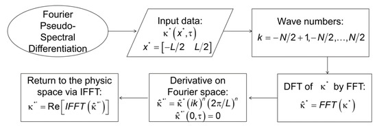
Figure 3.
Flowchart followed to perform the Fourier based pseudo-spectral (FPS) differentiation method.
Once obtained the n-order spatial derivatives of the interface position that intervene on the evolution equations (Equations (8)–(12)), the first order temporal derivative is determined using a forward finite difference, in such a way that the equation becomes explicit and the solution of next time step can be estimated.
3. Results and Discussion
This section has the objective of validating our unifying numerical framework. For this purpose, we evaluated some representative cases of the models studied here in order to compare the results obtained with the Fourier-based pseudo-spectral (FPS) differentiation method to those reported in the literature with other numerical techniques.
To solve the HAC model for gas–liquid elastic interfaces (Equation (8)) the authors used the Forward Euler (FE) method [16]. Here, we focused on those results that show the effect of the interfacial elasticity [26], encapsulated in the dimensionless parameter . The HAC model is evaluated in a geometry defined by , . The initial condition is defined by . First, Figure 4 shows the evolution of the interface radius over time at the center of the capillary for cases where values are (a) less than and (b) greater than the unit. In first case () snap-off occurs, but not in second case (). While in Figure 5, it is related to the interface profiles moments before the end of the simulation for different values of .

Figure 4.
Comparison of the interface radius evolution at the center of capillary throat () obtained with Forward Euler (FE)  and FPS
  methods for the HAC model (gas–liquid elastic interface). The results correspond to case: , , (a) (b) .
and FPS methods for the HAC model (gas–liquid elastic interface). The results correspond to case: , , (a) (b) .
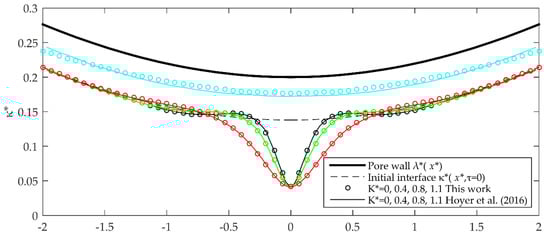
Figure 5.
Profiles of the gas–liquid elastic interfaces obtained through the HAC model, solved with FE ( ) and FPS (
 ) methods where , , and
  ;
;  ;
;  ;
;  .
.
) and FPS () methods where , , and ; ; ; .
The solutions reported for the GR model [10] (gas–liquid interfaces), represented by Equation (10), were obtained using the GFE method, which are compared to those obtained by this work with the FPS method. Figure 6 shows the interface evolution profiles at different dimensionless times, for the same geometry used on the previous case but with initial conditions defined by . In the case of a straight capillary, the GR model is evaluated for a dimensionless initial film thickness and a dimensionless wavelength of fastest growing disturbance of . In Figure 7 we compared the evolution of the interface profiles reported by Gauglitz and Radke [9] using the Galerkin FE method, to those obtained with the MATLAB “pdepe” solver by Zhang et al. [13] and to the results of this work applying the FPS method.

Figure 6.
Gas–liquid interface evolution profiles with Galerkin-FE ( ) and FPS (
 ) methods for the Gauglitz and Radke (GR) model are compared. The results shown correspond to: , and at different unidimensional times:
  ;
;  ;
;  .
.
) and FPS () methods for the Gauglitz and Radke (GR) model are compared. The results shown correspond to: , and at different unidimensional times: ; ; .

Figure 7.
Profiles that show the evolution of the gas-liquid interface obtained by solving the GR model for straight capillaries, with the FPS method ( ) and its comparison with those reported by Gauglitz and Radke (1988) with Galerkin-FE (
 ) and Zhang et al. (2016) with MATLAB solver (
 ), for and . The profiles are shown for:
  ;
;  ;
;  .
.
) and its comparison with those reported by Gauglitz and Radke (1988) with Galerkin-FE () and Zhang et al. (2016) with MATLAB solver (), for and . The profiles are shown for: ; ; .
Regarding the viscous core fluid case, the BD model for liquid–liquid interfaces (Equation (12)) is first evaluated for a base case defined by , , , and different values of . This base case is used by the BD model authors to validate the numerical solutions obtained with the MOL implemented on Mathematica [18] through the comparison of the solutions obtained by numerical simulations performed on CFD commercial codes. Here, we compare the results of Beresnev and Deng [17] with those obtained on this work with the FPS method (see Figure 8). The snap-off time for the cases that appear in Figure 8 are: (a) (b) (c) . Beresnev and Deng (Figure 3 in [14]) reported , respectively.
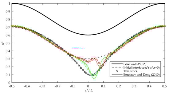
Figure 8.
Liquid–liquid interface profiles obtained with the BD model solved with the MOL ( ) and the FPS (
 ) methods. The results correspond to the simulations performed with , , , and the geometric slopes:
  ;
;  ;
;  .
.
) and the FPS () methods. The results correspond to the simulations performed with , , , and the geometric slopes: ; ; .
After these comparisons, the BD model is evaluated for two specific cases depicted in Figure 9. The first inspects a geometric break-up criterion (Equation (6) in [23]); the geometric slope overcomes the upper limit of such criterion () with the rest of parameters maintained. This means that, in theory, the snap-off is inhibited. In one of the profiles shown in Figure 9 it may be appreciated that the FPS reproduces this situation, i.e., snap-off does not occur and the wetting liquid film decreases its thickness. The second case in Figure 9 corresponds to a reversed viscosity ratio, that is the most viscous liquid is now the wetting phase, thus: . The rest of the parameters are those of the base case, but with and ; this last parameter corresponds with the geometry in case of Figure 8c. In fact, this case tries to demonstrate that even in most unfavorable conditions for drop breakup (displaced wetting phase more viscous than the non-wetting phase and a low flow regime), the breakup occurs if the geometrical criterion of rupture is met. Although, it should be noted that the effect of these “unfavorable” flow conditions is reflected on the snap-off time ; since this is increased from to . Beresnev and Deng (Figure 3c and Figure 7 in [14]) report for these cases , respectively.
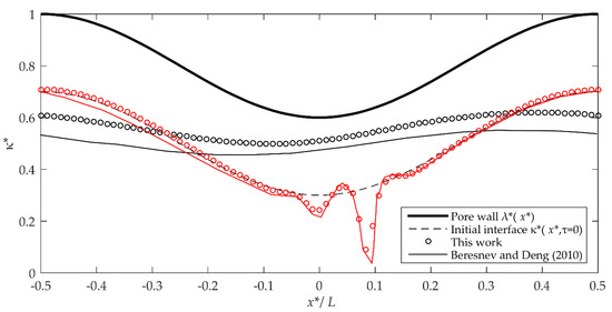
Figure 9.
Liquid–liquid interface profiles obtained with the BD model solved with the MOL ( ) and the FPS (
 ) methods. The results correspond to the simulations performed with , and
  ; , and
  . In both cases, and .
) and the FPS () methods. The results correspond to the simulations performed with , and ; , and . In both cases, and .
As it may be observed on the series of Figure 4, Figure 5, Figure 6, Figure 7, Figure 8 and Figure 9, there is an acceptable agreement between the results of the snap-off dynamics obtained in this work and those reported on the literature. The small deviations on snap-off time and form of the interface can be related with the arbitrary definition of breakup time. Regarding the differences in the interface evolution of inviscid and viscous core fluid, it should be noted that in the first case the forms of the interface are axisymmetric, in addition to the fact that a single breaking point is observed (Figure 5 and Figure 6). While in the second case the results show a more varied interface dynamics, both in non-symmetrical forms and in the presence, in some configurations, of more than one breaking point (Figure 8 and Figure 9). This can be explained by the high non-linearity of the BD model (Equation (12)) and the periodic boundary conditions imposed (Equation (19)).
It is important to remark that the small-slope based models assume , so the smaller , the better the approximation. On Beresnev et al. (Table III in [23]), for example, it is clear that the order of the ratio between the theoretical and experimental snap-off times decreases for greater values of the slope wall; recalling the assumption of small slope built into the theory. This situation is observed too if we compare the snap-off time () of the cases of Figure 8 with those reported of CFD experiments () (Figure 3 in [14]); the ratios for are (a) (b) (c) , respectively.
4. Conclusions
The snap-off mechanism in circular capillaries was studied here from a theoretical approach. Particularly, we focused on the models reported that are based on the small-slope approach [9,10] for gas–liquid elastic, gas–liquid and liquid–liquid interfaces, mainly: GR, HE and BD models [9,10,16,17]. Although the rheology of each interface implies important considerations on the formulation of the models, their structures are similar: evolution equations described by highly nonlinear partial differential equations of fourth order in space and first order in time (Equations (8)–(12)). According to the reviewed literature, different mathematical techniques have been employed to solve such models, from the Forward Euler simple method to the use of powerful solvers implemented in commercial software.
We thus present a unifying framework to solve the group of referred models. This framework is based on Fourier pseudo-spectral (FPS) differentiation method and uses the Fast Fourier Transform (FFT) and the inverse FFT (IFFT), as is schematized in Figure 3. To demonstrate the effectiveness of our framework we evaluate some of the most representative model cases studied here and compared the results that we obtained with those reported in the literature. As it can be seen in Figure 4, Figure 5, Figure 6, Figure 7, Figure 8 and Figure 9 there is an acceptable agreement between the results of the snap-off dynamics (shape of the interface profile and snap-off time). The fact that the FPS differentiation method turns out to be suitable for the solution of the models studied here, may be related with the periodic domain of the problem, which results adequate to implement the trigonometric interpolant used in the pseudo-spectral method.
Finally, it is important to mention that despite the fact that the snap-off phenomenon was studied here by mathematical modelling, most of the exposed models (except the HAC model) have been validated experimentally [9,10,13,27,28]. Furthermore, it should be noted that a series of simplifications are made on the models’ formulations, so future research might focus on overcoming these limitations.
Author Contributions
Conceptualization, A.Q., E.G.-S., and C.F.; methodology, A.Q., C.F., C.C., and E.G.-S.; software, A.Q. and C.M.; investigation, A.Q.; writing—original draft preparation, A.Q.; writing—review and editing, A.Q., C.F. and C.C. All authors have read and agreed to the published version of the manuscript.
Funding
This research was funded by the National Council for Science and Technology (CONACYT) in Mexico, grant number 25345.
Conflicts of Interest
The authors declare no conflict of interest.
References
- Peña, T.; Carvalho, M.; Alvarado, V. Snap-off of a liquid drop immersed in another liquid flowing through a constricted capillary. Alche J. 2009, 55, 1993–1999. [Google Scholar] [CrossRef]
- Deng, W.; Cardenas, M.B.; Bennett, P.C. Extended Roof snap-off for a continuous nonwetting fluid and an example case for supercritical CO2. Adv. Water Resour. 2014, 64, 34–46. [Google Scholar] [CrossRef]
- Tsai, T.; Miksis, M.J. Dynamics of a drop in a constricted capillary tube. J. Fluid Mech. 1994, 274, 197–217. [Google Scholar] [CrossRef]
- Kouris, C.; Tsamopoulos, J. Core-annular flow in a periodically constricted circular tube. Part 2. Nonlinear dynamics. J. Fluid Mech. 2002, 470, 181–222. [Google Scholar] [CrossRef]
- Armstrong, R.; Berg, S.; Dinariev, O.; Evseev, N.; Klemin, D.; Koroteev, D.; Safonov, S. Modeling of pore-scale two-phase phenomena using density functional hydrodynamics. Transp. Porous Med. 2016, 112, 577–607. [Google Scholar] [CrossRef]
- Roman, S.; Abu-Al-Saud, M.O.; Tokunaga, T.; Wan, J.; Kovscek, A.R.; Tchelepi, H.A. Measurements and simulation of liquid films during drainage displacements and snap-off in constricted capillary tubes. J. Colloid Interface Sci. 2017, 507, 279–289. [Google Scholar] [CrossRef]
- Starnoni, M.; Pokrajac, D. Numerical study of the effects of contact angle and viscosity ratio on the dynamics of snap-off through porous media. Adv. Water Resour. 2018, 111, 70–85. [Google Scholar] [CrossRef]
- Meng, Y.; Li, X.; He, M.; Jiang, M. A semi-analytical model research of liquid collar shape and coalescence in pore throat during snap-off. Arab. J. Geosci. 2019, 12, 468. [Google Scholar] [CrossRef]
- Gauglitz, P.; Radke, C. An extended evolution equation for liquid film breakup in cylindrical capillaries. Chem. Eng. Sci. 1988, 43, 1457–1465. [Google Scholar] [CrossRef]
- Gauglitz, P.; Radke, C. The dynamics of liquid film breakup in constricted cylindrical capillaries. J. Colloid Interface Sci. 1990, 134, 14–40. [Google Scholar] [CrossRef]
- Middleman, S. Modeling Axisymmetric Flows: Dynamics of Films, Jets, and Drops; Academic Press: San Diego, CA, USA, 1995. [Google Scholar]
- Hammond, P. Nonlinear adjustment of a thin annular film of viscous fluid surrounding a thread of another within a circular cylindrical pipe. J. Fluid Mech. 1983, 137, 363–384. [Google Scholar] [CrossRef]
- Zhang, H.; Nikolov, A.; Feng, J.; Wasan, D. The dynamics of the annular liquid layer inside a cylindrical capillary. Phys. Fluids 2016, 28, 024107. [Google Scholar] [CrossRef]
- Skeel, R.D.; Berzins, M. A method for the spatial discretization of parabolic equations in one space variable. Siam J. Sci. Stat. Comput. 1990, 11, 1–32. [Google Scholar] [CrossRef]
- Shampine, L.F.; Reichelt, M.W. The matlab ode suite. SIAM J. Sci. Comput. 1997, 18, 1–22. [Google Scholar] [CrossRef]
- Hoyer, P.; Alvarado, V.; Carvalho, M. Snap-off in constricted capillary with elastic interface. Phys. Fluids 2016, 28, 012104. [Google Scholar] [CrossRef]
- Beresnev, I.; Deng, W. Theory of breakup of core fluids surrounded by a wetting annulus in sinusoidally constricted capillary channels. Phys. Fluids 2010, 22, 012105. [Google Scholar] [CrossRef]
- Knapp, R. A Method of Lines Framework in Mathematica1. JNAIAM 2008, 3, 43–59. [Google Scholar]
- Bretherton, F. The motion of long bubbles in tubes. J. Fluid Mech. 1961, 10, 166–188. [Google Scholar] [CrossRef]
- Beresnev, I.; Gaul, W.; Vigil, R.D. Thickness of residual wetting film in liquid-liquid displacement. Phys. Rev. E 2011, 84, 026327. [Google Scholar] [CrossRef]
- Deng, W.; Balhoff, M.; Cardenas, M.B. Influence of dynamic factors on nonwetting fluid snap-off in pores. Water Resour. Res. 2015, 51, 9182–9189. [Google Scholar] [CrossRef]
- Trefethen, L.N. Spectral Methods in Matlab; SIAM: Philadelphia, PA, USA, 2000. [Google Scholar]
- Weideman, J.A.; Reddy, S.C. A MATLAB differentiation matrix suite. ACM Trans. Math. Softw. 2000, 26, 465–519. [Google Scholar] [CrossRef]
- Cooley, J.W.; Tukey, J.W. An algorithm for the machine calculation of complex Fourier series. Math. Comput. 1965, 19, 297–301. [Google Scholar] [CrossRef]
- Csáti, Z. Fourier Differentiation. Available online: http://www.mathworks.com/matlabcentral/fileexchange (accessed on 15 August 2020).
- Hoyer, P.; Alvarado, V. Stability of liquid bridges with elastic interface. RSC Adv. 2017, 7, 49344–49352. [Google Scholar] [CrossRef]
- Beresnev, I.; Gaul, W.; Vigil, R.D. Forced instability of core-annular flow in capillary constrictions. Phys. Fluids 2011, 23, 072105. [Google Scholar] [CrossRef]
- Gauglitz, P.; St. Laurent, C.; Radke, C. Experimental determination of gas-bubble breakup in a constricted cylindrical capillary. Ind. Eng. Chem. Res. 1988, 27, 1282–1291. [Google Scholar] [CrossRef]
Publisher’s Note: MDPI stays neutral with regard to jurisdictional claims in published maps and institutional affiliations. |
© 2020 by the authors. Licensee MDPI, Basel, Switzerland. This article is an open access article distributed under the terms and conditions of the Creative Commons Attribution (CC BY) license (http://creativecommons.org/licenses/by/4.0/).