1. Introduction
The Markowitz mean-variance portfolio selection problem has been initially considered in [
1] in a single-period model. In this framework, investement decision rules are made according to the objective of maximizing the expected return of the portfolio for a given financial risk quantified by its variance. The Markowitz portfolio is widely used in the financial industry due to its intuitive formulation and the fact that it produces, by construction, portfolios with high Sharpe ratios (defined as the ratio of the average of portfolio returns over their volatility), which is a key metric used to compare investment strategies.
The mean-variance criterion involves the expected terminal wealth in a nonlinear way due to the presence of the variance term. In a continuous-time dynamic setting, this induces the so-called time inconsistency problem and prevents the direct use of the dynamic programming technique. A first approach, from [
2], consists of embedding the mean-variance problem into an auxiliary standard control problem that can be solved by using stochastic linear-quadratic theory. Some more recent approaches rely on the development of stochastic control techniques for McKean–Vlasov (MKV) type control problems. MKV control problems are problems in which the equation of the state process and the cost function involve the law of this process and/or the law of the control, possibly in a non-linear way. The mean-variance portfolio problem in continuous-time is a McKean–Vlasov control problem of the linear-quadratic type. The state diffusion, which represents the wealth of the portfolio, involves the state process and the control in a linear way while the cost involves the terminal value of the state and the square of its expectation due to the variance criterion. In [
3], the authors solved the mean-variance problem as a McKean–Vlasov control problem by deriving a version of the Pontryagin maximum principle. More recently, [
4] developed a general dynamic programming approach for the control of MKV dynamics and applied it for the resolution of the mean-variance portfolio selection problem. In [
5], the mean-variance problem is viewed as the MKV limit of a family of controlled many-component weakly interacting systems. These prelimit problems are solved by standard dynamic programming, and the solution to the original problem is obtained by passage to the limit.
A frequent criticism addressed to the mean-variance allocation is its sensitivity to the estimation of expected returns and covariance of the stocks and the risk of a poor out-of-sample performance. Several solutions to these issues have been considered. An approach consists of using a more sophisticated model than the Black–Scholes model, in which the parameters are stochastic or ambiguous and to take decisions under the worst-case scenario over all conceivable models. Robust mean-variance problems have thus been considered in the economic and engineering literature, mostly on single-period or multi- period models; see, e.g., [
6,
7,
8]. In a continuous-time setting, ref. [
9] have developed a robust approach by studying the mean-variance allocation with a market model where the model uncertainty affects the covariance matrix of multiple risky assets. In [
10], the authors study the problem of utility maximization under uncertain parameters in a model where the parameters of the model do not evolve freely within a given range, but are constrained via a penalty function. Let us also mention uncertain volatility models in [
11,
12] for robust portfolio optimization with expected utility criterion. Another approach is to rely on the shrinking of the portfolio weights or of the wealth invested in each risky asset in order to obtain a more sparse or more stable portfolio. In [
13], the authors find single-period portfolios that perform well out-of-sample in the presence of estimation error. Their framework deals with the resolution of the traditional minimum-variance problem with the additional constraint that the norm of the portfolio-weight vector must be smaller than a given threshold. In [
14], the authors study a one-period mean-variance problem in which the mean-variance objective function is regularized with a weighted elastic net penalty. They show that the use of this penalty can be justified by a robust reformulation of the mean-variance criterion that directly accounts for parameter uncertainty. In the same spirit, in [
15],
-norm regularized models are used to seek near-optimal sparse portfolios.
In this paper, we investigate the mean-variance portfolio selection in continuous time with a tracking error penalization. This penalization represents the distance between the optimized portfolio composition and the composition of a reference portfolio with the same wealth but fixed weights that have been chosen in advance. Typical reference portfolios widely used in the financial industry are the equal weights, the minimum variance and the equal risk contribution (ERC) portfolios. The equal weights portfolio studied, e.g., in [
16], is a portfolio where all the wealth of the investor is invested in risky assets and divided equally between the different assets. The minimum variance portfolio is a portfolio where all the wealth is invested in risky assets and portfolio weights are optimized in order to attain the minimal portfolio volatility. The ERC portfolio, presented in [
17] and in the monography [
18], is totally invested in risky assets and optimized such that the contributions of each asset to the total volatility of the portfolio are equal. The mix of the mean-variance and of this tracking error criterion can be interpreted in two different ways: (i) From a first viewpoint, it is a procedure to regularize and robustify the mean-variance allocation. By choosing reference portfolio weights which are not based on the estimation of market parameters, or which are less sensible to estimation error, the allocation obtained is more robust to parameters estimation error than the standard mean-variance one. (ii) From a second viewpoint, this optimization permits to mimic an allocation corresponding to the reference portfolio weights while improving its Sharpe ratio via the consideration of the mean-variance criterion.
We tackle this problem as a McKean–Vlasov linear-quadratic control problem and adopt the approach developed in [
19], where the authors give a general method to solve this type of problems by means of a weak martingale optimality principle. We obtain explicit solutions for the optimal portfolio strategy and value function, and provide asymptotic expansions of the portfolio strategy and efficient frontier for small values of the portfolio tracking error penalization parameter. We then compare the Sharpe ratios obtained by the standard mean-variance portfolio, the penalized one and the reference portfolio in two different ways. First, we compare these performances on simulated market data with misspecified market parameters. Different magnitudes of parameter misspecifications are used to illustrate the impact of the parameter estimation error on the performance of the different portfolios. In a second time, we compare the performances of these portfolios on a backtest based on historical market data. In these tests, we shall consider three reference portfolios cited above: the equal weights, the minimum variance and the equal risk contribution (ERC) portfolios. Finally, we will also consider the case where the reference portfolio weights are all equal to zero. This case corresponds to a shrinking of the wealth invested in the different risky assets along the investment horizon.
The rest of the paper is organized as follows.
Section 2 formulates the mean-variance problem with tracking error. In
Section 3, we derive explicit solutions for this control problem and provide expansion of this solution for small values of the tracking error penalization parameter.
Section 4 is devoted to the applications of those results and to the comparison of the mean-variance, penalized and reference portfolio for the different reference portfolios presented above. We show the benefit of the penalized portfolio compared to the standard mean-variance portfolio and the different reference portfolios on simulated and historical data in terms of Sharpe ratio and the lower sensitivity of the penalized portfolio to parameter estimation error.
2. Results
Throughout this paper, we fix a finite horizon
T∈
, and a complete probability space
on which a standard
-adapted
d-dimensional Brownian motion
W=
is defined. We denote by
the set of all
-valued, measurable stochastic processes
adapted to
such that
. We consider a financial market with price process
, composed of one risk-free asset, assumed to be constant equal to one, i.e.,
≡ 1, and
d risky assets on a finite investment horizon
. These assets price processes
satisfy the following stochastic differential equation:
where
is the appreciation rate, and
is the volatility matrix of the
d stocks. We denote by
the covariance matrix. Throughout this paper, we will assume that the following nondegeneracy condition holds
for some
, where
is the
identity matrix.
Let us consider an investor with total wealth at time
denoted by
, starting from some initial capital
> 0. It is assumed that the trading of shares takes place continuously and transaction cost and consumptions are not considered. We define the set of admissible portfolio strategies
=
as
where
represents the total market value of the investor’s wealth invested in the
ith asset at time
t. The dynamics of the self-financed wealth process
X=
associated to a portfolio strategy
∈
is then driven by
Given a risk aversion parameter
, and a reference weight
∈
, the objective of the investor is to minimize over admissible portfolio strategies a mean-variance functional to which is added a running cost:
This running cost represents a running tracking error between the portfolio composition of the investor and the reference composition of a portfolio of same wealth and constant weights . The matrix is symmetric positive definite and is used to introduce an anisotropy in the portfolio composition penalization. The penalization , which we will call “tracking error penalization", is introduced in order to ensure that the portfolio of the investor does not move away too much from this reference portfolio with respect to the distance .
The mean-variance portfolio selection with tracking error is then formulated as
and an optimal allocation given the cost
will be given by
We complete this section by recalling the solution to the mean-variance problem when there is no tracking error running cost, and which will serve later as benchmark for comparison when studying the effect of the tracking error with several reference portfolios.
Remark 1 (Case of no tracking error). When , it is known, see e.g., [2] that the optimal mean-variance strategy is given bywhere is the wealth process associated to . The vector , which depends only on the model parameters of the risky assets, determines the allocation in the risky assets. In the sequel, we study the quantitative impact of the tracking error running cost on the optimal mean-variance strategy.
3. Solution Allocation with Tracking Error
Our main theoretical result provides an analytic characterization of the optimal control to the mean-variance problem with tracking error.
Theorem 1. There exist a unique pair solution to the system of ODEswhere . The optimal control for problem (3) is then given bywithand is the wealth process associated to . Moreover, we have Proof. Given the existence of a pair
solution to (
5), the optimality of the control process in (
6) follows by the weak version of the martingale optimality principle as developed in [
19]. The arguments are recalled in
Appendix A.
Here, let us verify the existence and uniqueness of a solution to the system (
5).
- (i)
We first consider the equation for
K, which is a scalar Riccati equation. The equation for
K is associated to the standard linear-quadratic stochastic control problem:
where
is the controlled linear dynamics solution to
By a standard result in control theory ([
20] Ch. 6, Thm. 6.1, 7.1, 7.2), there exists a unique solution
to the first equation of system (
5) (more,
if
is nonzero). In this case, we have
.
- (ii)
Given
K, we consider the equation for
. This is also a scalar Riccati equation. By the same arguments as for the
K equation, there exists a unique solution
to the second equation of (
5), provided that
for some
. We already have that
. From the fact that
, together with the nondegeneracy condition on the matrix
, we have that
. Since
> 0, and under the nondegeneracy condition of matrix
, we can use the Woodbury matrix identity to obtain
- (iii)
Given
, the equation for
Y is a linear ODE, whose unique continuous solution is explicitly given by
- (iv)
Given
,
R can be directly integrated into
□
We can see from the expression of the optimal control (
6) that the allocation in the risky assets has two components. One component is determined by the vector
with leverage
, and the second one by the vector
with leverage
. Computing the average wealth
=
associated to
, we can express the control
as a function of the initial wealth of the investor
and the current wealth
where we set
and
.
Remark 2. In the case when Γ
is the null matrix, Γ
= , we see that the first component of the optimal control (7) vanishes,and the system of ODES (5) of becomeswhich yields the explicit forms We get , and . The first line of the optimal control equation vanishes and the second line can be rewritten as Computing the integral in this expression, we recover the optimal control of the classical mean-variance problem (4). Remark 3(Limit offor). If we consider Γ
in the form , the optimal control can be rewritten as We show in Appendix D that and are bounded functions of the penalization parameter γ, thus . We rewrite asand we get that . Thus the second term of (8) vanishes and we getwhich corresponds to the reference portfolio. Remark 4(Expansion for). We take . Since the covariance matrix Σ
is symmetric, there exists an invertible matrix and a diagonal matrix such that . We can then rewrite the matrix aswithwhere is the i-th diagonal value of the diagonal matrix D. From the nondegeneracy condition of the covariance matrix, we have . As , we want to write the Taylor expansion of the diagonal elements of the inverse matrix equal to . We have that , thus . We can then write the Taylor expansion of the matrix askeeping only the terms up to the linear term in γ. Putting this expression in the differential equation of K, and keeping only the terms up to the linear term in γ, we get the differential equationwhere we set . We look for a solution to this equation of the form Putting this expression in the differential Equation (9), we get two differential equations, for the leading order and the linear order in γ respectivelywhich yield the explicit solutionwhere is the solution to the differential equation in the unpenalized case. From the expansion for K, we can write the expansion of the differential equation for Λ
up to the linear term in γ. We use the expansionand we get the following expansion of the differential equation of Λ
As before, we look for a solution of this differential equation of the form Plugging this expression into the Equation (10), we get the two following differential equations The first differential equation yields the solution . Replacing by this value in the second differential equation, we get the equationand obtain the solution We can also compute the first order expansion of where we setand we have The last expansion we need to compute before rewritting the optimal control is the expansion of . We can rewritewith As shown in Appendix B, we can rewrite the optimal controlwhere we set , and with We see that for , we recover the classical mean-variance optimal control. For non-zero values of γ, we see that a mix of three different portfolio allocations is obtained. The weight of the allocation is modified and two allocations and appear with weights and .
From this expansion of the control , we can compute the first order asymptotic expansion in γ of the equation giving the relation between the variance of the terminal wealth of the portfolio and its expectation. In the classical mean-variance case, this equation is called the efficient frontier formula. As shown in Appendix C, with the tracking error penalization, the first order asymptotic expansion in γ gives The leading order term corresponds to the efficient frontier equation of the classical mean-variance allocation computed in [2], and thus for , we recover this classical result. The linear term in γ contains contributions of the three perturbative allocations. A modification of "leverage" of the original mean-variance allocation and two different allocations and . 4. Applications and Numerical Results
In this section, we apply the results of the previous section and study the allocation obtained by considering four different static portfolios as reference. First, we shall study these allocations on simulated data, in the case of misspecified parameters. The misspecification of parameters means that the market parameters used to compute the portfolio allocations are different from the ones driving the stocks prices. This study allows us to estimate the impact of the estimation error on the portfolio performance. For a second time, we perform a backtest and run the different portfolios on real market data. To simplify the presentation, we will assume now that the tracking error penalization matrix is in the form
with
. With this simplification, we have
and we can rewrite the system of ODEs (
5) and the optimal control (
6) as
and
where
We will consider three different classical allocations as reference portfolio.
Equal-weights portfolio: in this classical equal-weights portfolio, the same capital is invested in each asset, thus
where
d is the number of risky assets considered and
is the vector of ones.
Minimum variance portfolio: the minimum variance portfolio is the portfolio which achieves the lowest variance while investing all its wealth in the risky assets. The weight vector of this portfolio is equal to
These weights correspond to the one-period Markowitz portfolio when every asset expected return is taken equal to 1. In that case, only the portfolio variance is relevant and is minimized during the optimization process.
ERC portfolio: the equal risk contributions (ERC) portfolio, presented in [
17] and in the monograph [
18] is constructed by choosing a risk measure and computing the risk contribution of each asset to the global risk of the portfolio. When the portfolio volatility is chosen as the risk measure, the principle of the ERC portfolio lays in the fact that the volatility function satisfies the hypothesis of Euler’s theorem and can be reduced to the sum of its arguments multiplied by their first partial derivatives. The portfolio volatility
of a portfolio with weights vector
can then be rewritten as
The term under the sum
, corresponding to the
i-th asset, can be interpreted as the contribution of this risky asset to the total portfolio volatility. The equal risk contribution allocation is then defined as the allocation in which these contributions are equal for all the risky assets of the portfolio,
for every
. The equal risk contribution allocation is thus obtained when the portfolio weights
are given by
With this risk measure, the ERC portfolio weights can be expressed in a closed-form only in the case where the correlations between every couple of stocks are equal, that is
, with the additional assumption that
. Under these assumptions, and with the constaint that
, the weights of this portfolio are equal to
where
is the volatility of the
i-th asset.
In the general case, the weights of the ERC portfolio do not have a closed form and must be computed numerically by solving the following optimization problem
Control shrinking (zero portfolio): this is the portfolio where all weights are equal to zero, for all i. This case corresponds to a shrinking of the controls of the penalized allocation, in the same spirit as the shrinking of regression coefficients in the Ridge regression (or Tikhonov regularization).
4.1. Performance Comparison with Monte Carlo Simulations
In this section we compare, for each reference portfolio, the classical dynamic mean-variance allocation, the reference portfolio and the “tracking error" penalized portfolio. In a real investment situation, expected return and covariance estimates are noisy and biased. Thus, in order to compare the three portfolios and observe the impact of adding a tracking error penalization in the mean-variance allocation, we will run Monte Carlo simulations, assuming that the real-world expected returns
and covariances
are equal to reference expected returns
and covariances
plus some noise:
with the volatilties
and correlations
and
where the covariance matrix
is obtained from
and
. The noise follows a standard normal distribution
and
is its magnitude. We use Monte Carlo simulations to estimate the expected Sharpe ratio of each portfolio, equal to the average of the portfolio daily returns
R divided by the standard deviation of those returns:
.
We consider an investment horizon of one year, with 252 business days and a daily rebalancing of the portfolio. The risk aversion parameter
is chosen so that the targeted annual return of the classical mean-variance allocation is equal to
, thus
according to [
2]. The initial wealth of the investor
is chosen equal to 1 and we choose the penalization parameter
. Indeed, as the value of
depends on the value of the stocks expected return and covariance matrix and on the targeted return, and can be very big, we express
a function of this
in order for the penalization to be relevant and non-negligible.
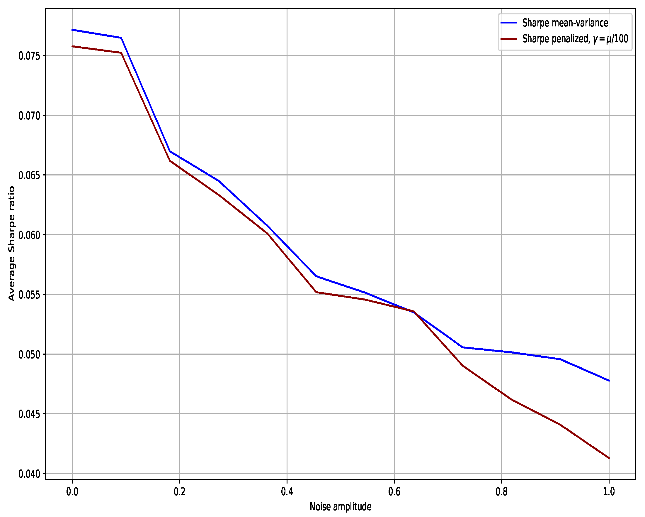
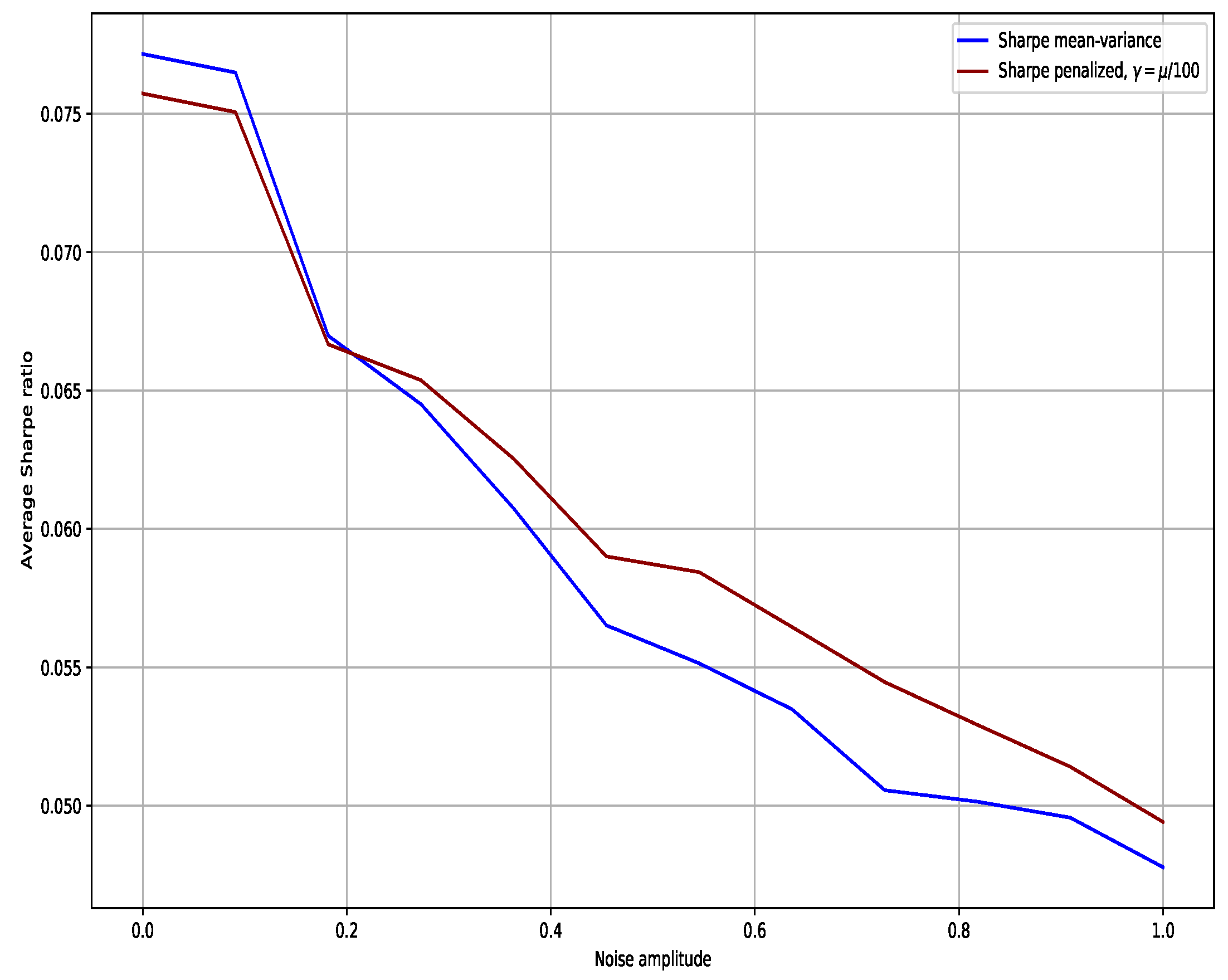
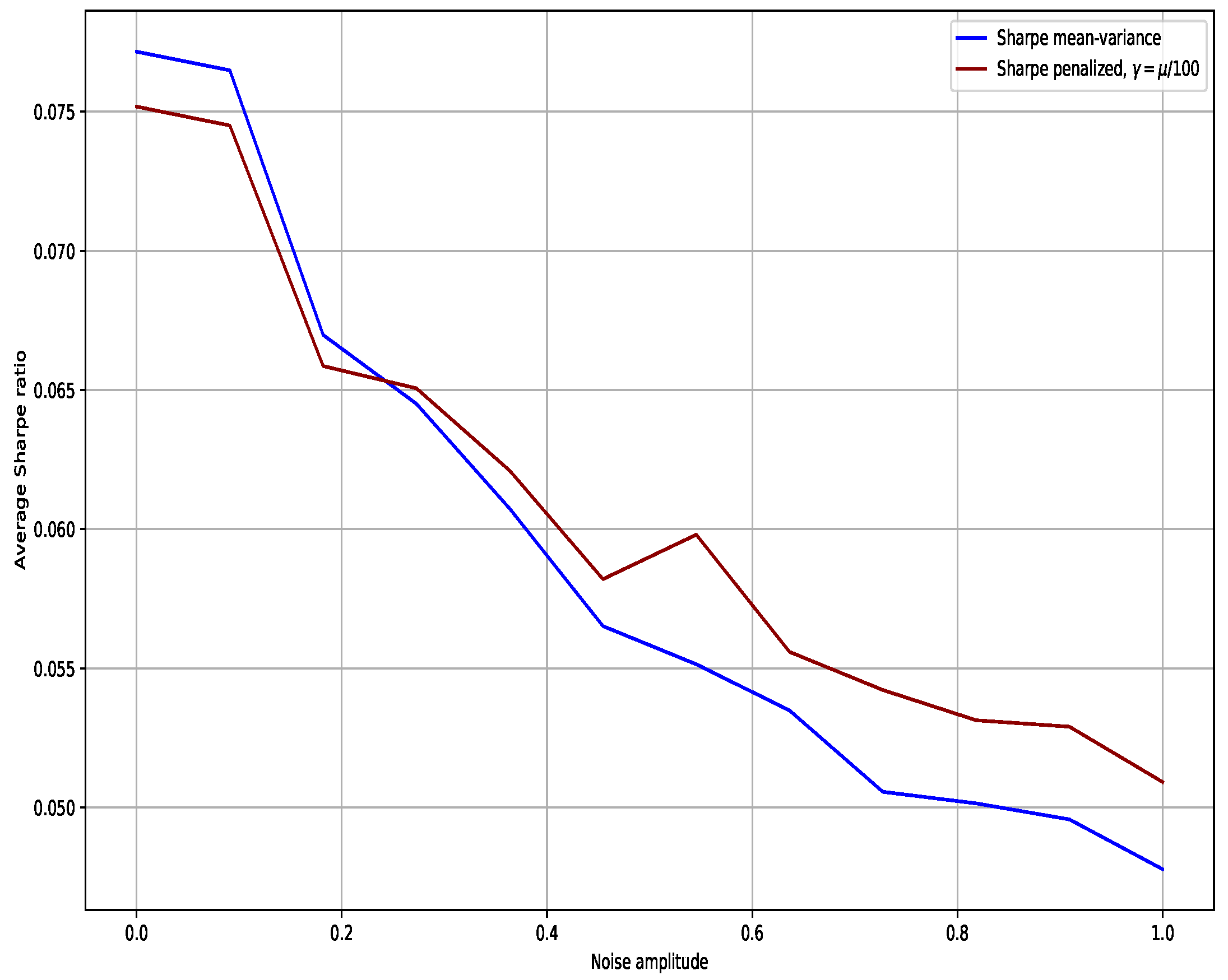
For each reference portfolio, we compare the reference portfolio, the classical mean-variance allocation and the penalized one for values of noise amplitude ranging from 0 to 1. For each value of , we run 2000 scenarios and we plot the graphs of the average Sharpe ratio as a function of .
On the
Figure 1,
Figure 2,
Figure 3 and
Figure 4, we can see that in the four cases, the mean-variance and the penalized portfolios are superior to the reference. In the case where the equal weights portfolio is chosen as reference, the penalized portfolio’s Sharpe ratio is lower than the mean-variance one for small values of
. For
greater than approximately 0.25, the penalized portfolio’s Sharpe ratio becomes larger and the gap with the mean-variance’s Sharpe tends to increase with
. The same phenomenon occurs in the case where the ERC portfolio is chosen as reference, with a smaller gap between the mean-variance and penalized portfolios’ Sharpe ratios. When the minimum variance portfolio is chosen as reference, the penalized portfolio’s Sharpe ratio is lower than the one of the mean-variance portfolio for all
in the interval
. This is certainly due to the sensitivity of the minimum variance portfolio to the estimator of the covariance matrix. Finally, in the case of the control shrinking, the Sharpe ratio of the penalized portfolio is significantly higher that the Sharpe ratio of the mean-variance portfolio, for every value of the noise amplitude
in the interval
.
Equal-weights reference portfolio
Minimum-variance reference portfolio
ERC reference portfolio
Control shrinking (zero reference)
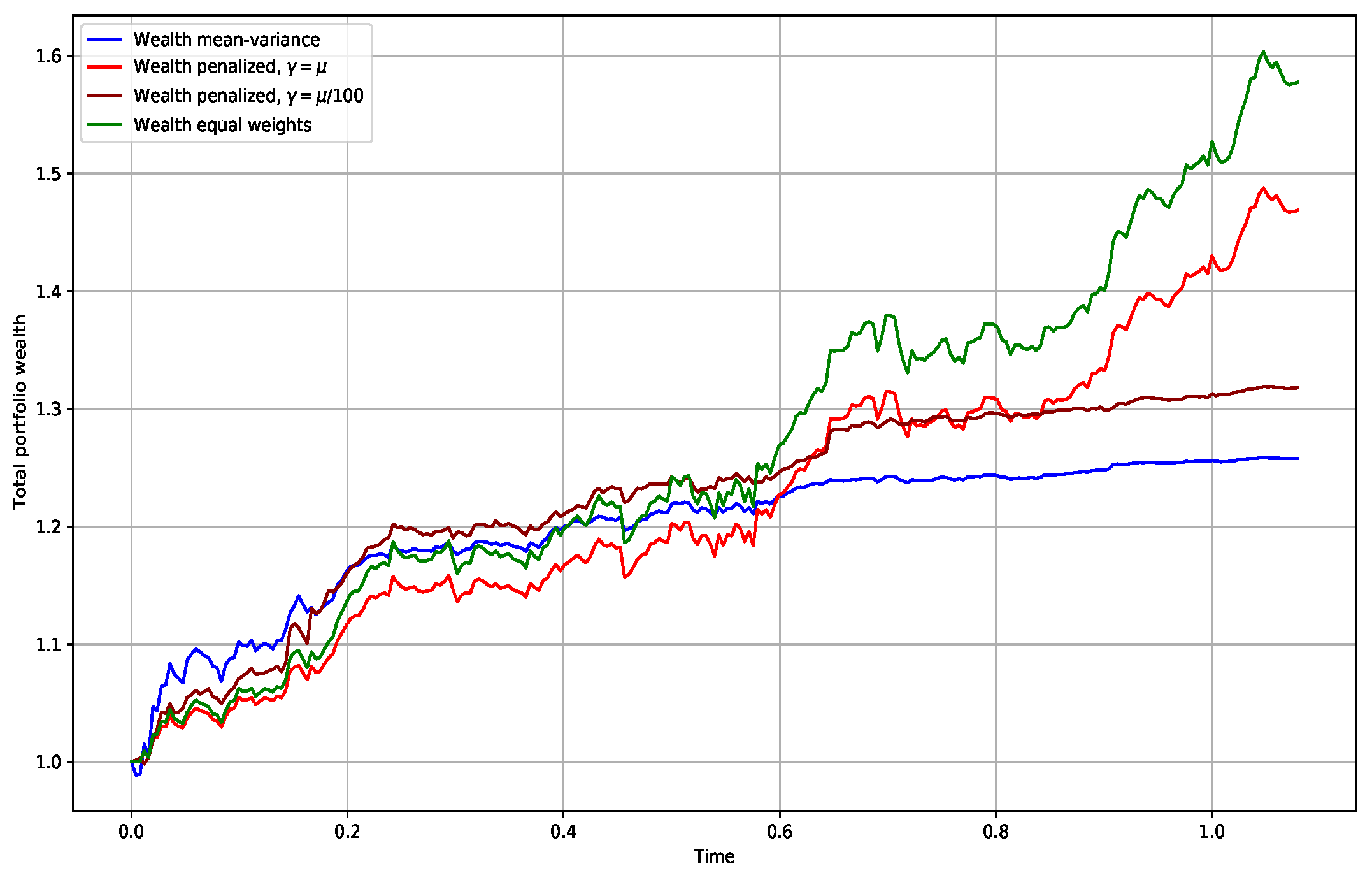
4.2. Performance Comparison on a Backtest
We now compare the different allocations on a backtest based on adjusted close daily prices available on Quandl between 2013-09-03 and 2017-12-28 for four stocks: Apple, Microsoft, Boeing and Nike. Here we chose a value of which corresponds to an annual expected return of . In our example, we express again as a function of and we consider two different values, and .
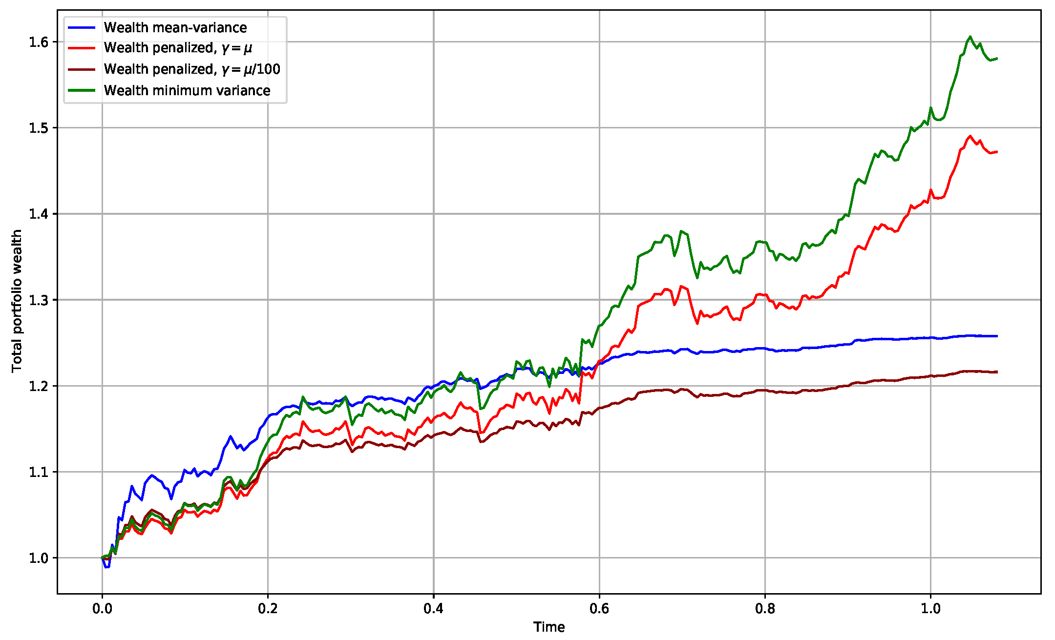
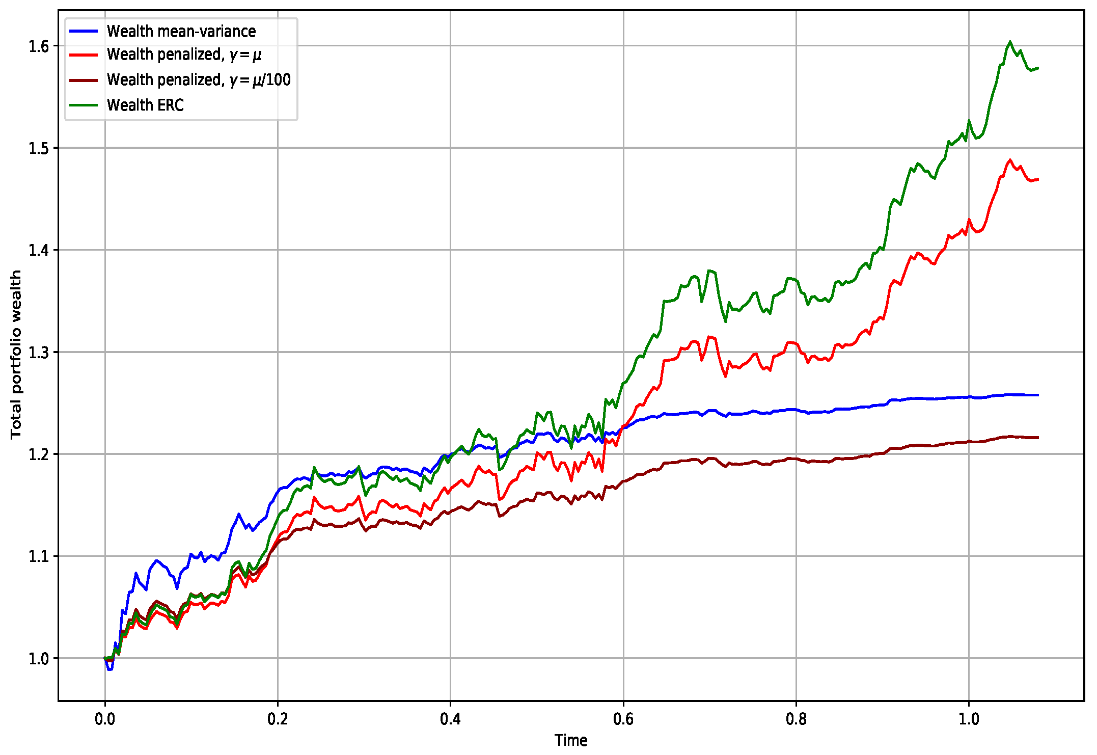
Figure 5,
Figure 6 and
Figure 7 show the total wealth of the four different portfolios, mean-variance, reference and the penalized portfolio with the big and the small penalization as a function of time. On these graphs we observe that, at the beginning of the investment horizon, the mean-variance allocation has the largest wealth increase, hence the largest leverage. As the wealth of this portfolio attains the target wealth, expressed as
in the mean-variance control Equation (
4), its leverage decreases and its wealth curve flattens. The same phenomenon occurs for the penalized allocation with large penalization parameter
. In this case, the high value of the penalization parameter keeps the penalized portfolio controls close to the ones of the mean-variance portfolio. On the contrary, the reference portfolios have constant weights and no target wealth. We can see that in each case the reference portfolio’s wealth keeps increasing over the entire horizon. The wealth of the penalized portfolio with penalization parameter
follows the wealth of these reference portfolio due to the small value of the tracking error penalization.
For these three reference portfolios, we observe that the penalized portfolio with penalization parameter
outperforms both the mean-variance and the reference portfolios in terms of Sharpe ratio whereas the penalized portfolio with penalization parameter
outperforms the mean-variance but underperforms the reference portfolio. This can be attributed to the larger weight of the mean-variance criterion with respect to the tracking error in the optimized cost (
2) with penalization parameter
.
Finally,
Figure 8 corresponds to the case of a reference portfolio with weights all equal to zero. This corresponds to a shrinking of the optimal control of the penalized portfolio. In that case, for a better visualization, we plot the total wealth of the mean-variance and penalized portfolios for penalization parameters
and
normalized by the standard deviation of their daily returns. On this graph, we can see that the normalized wealth of the two penalized portfolio is higher than the one of the mean-variance allocation. Similarly to the three precedent reference portfolios, the two penalized portfolios outperform the mean-variance allocation in terms of Sharpe ratio. As previously, we observe that the Sharpe ratio of the penalized portfolio with penalization parameter
is greater than the one with
, due to the larger weight of the mean-variance criterion in the functional cost.
Equal-weights reference portfolio
Minimum variance reference portfolio
ERC portfolio
Zero portfolio (shrinking)
5. Conclusions
In this paper, we propose an allocation method based on a mean-variance criterion plus a tracking error between the optimized portfolio and a reference portfolio of same wealth and fixed weights. We solve this problem as a linear-quadratic McKean–Vlasov stochastic control problem using a weak martingale approach. We then show using simulations that for a certain degree of market parameter misspecification and the right choice of reference portfolio, the mean-variance portfolio with tracking error penalization outperforms the standard mean-variance and the mean-variance allocations in terms of Sharpe ratio. Another backtest based on historical market data also shows that the mean-variance portfolio with tracking error outperforms the traditional mean-variance and the reference portfolios in terms of Sharpe ratio for the four reference portfolios considered.
Compared to the approaches of robust and bayesian optimization ([
9,
21]), the regularization of the mean-variance allocation by a tracking-error penalization offers a more intuitive and simple approach from the financial point of view as the specification of the reference portfolio has a clear operationnal meaning. The benchmark tracking with improvement of the Sharpe ratio is intrinsically linked to the method described in this article and is, by definition, absent of the two other approaches.
Depending on the penalization parameter , the choice of the reference portfolio plays an important role. If this reference portfolio is not agnostic and the computation of its weights is based on estimated market parameters, it will also be impacted by the parameter misspecification and the allocation will be more sensitive to estimation errors. The allocation would be more robust when an agnostic portfolio to market parameters, such as the equal-weights portfolio or the zero portfolio (control shrinking), is chosen as reference.
In our approach, the mean-variance criterion in the optimized cost function is based on estimated market parameters. Hence, while regularized by the tracking-error penalization, the allocation obtained still has a sensitivity to parameter misspecification. This constitutes a limitation compared to a robust optimization approach which optimizes the portfolio in the worst case scenario and is then unimpaired by parameter misspecification. Nevertheless, as the optimization of the mean-variance allocation with tracking error is based on estimators of the market parameters and not on a worst-case scenario, this allocation should outperform the robust approach for smaller values of parameter misspecification.
A potential direction for further studies would be to compare quantitatively the approach of the tracking error penalization with the robust optimization and the Bayesian approach. It would also be interesting to compare the method presented in this paper with Deep Learning based approaches such as the ones presented in [
22,
23].


