Identification Problem for Nonlinear Gao Beam

Abstract

This paper deals with the identification of coefficients in the nonlinear beam model which was first introduced by D. Y. Gao in 1996. For the identification of coefficients, an optimal control approach is used. The unknown coefficients are material parameters of the beam and play the role of the control variables. The existence of at least one solution of the optimal control problem is proved. For the studied problem the finite element approximation is provided. Finally some illustrative examples are introduced.

1. Introduction

Beams are important components in many engineering applications. The Euler- Bernoulli beam is the most popular model but it is linear and its validity is limited only to small deflections. For moderately large deflections it is better to use the nonlinear Gao beam model which was firstly introduced in [1] as a static problem and a few years latter as a dynamic model in [2]. This nonlinear beam model respects the original Euler–Bernoulli hypothesis—i.e., the straight lines orthogonal to the midsurface remain straight and orthogonal to it even after the deformation.

The paper is devoted to the identification of coefficients representing material properties for a static Gao beam model

$$EI{w}^{IV}-E\alpha {\left(w^{\prime }\right)}^2{w}^{″}+P\mu w^{″}=f$$

(1)

where $w=w\left(x\right)$ is a deflection of the beam, E stands for Young’s modulus, I is the constant area moment of inertia while functions $\alpha =3tb(1-{\nu }^2)$, $\mu =(1+\nu )(1-{\nu }^2)$ and $f=(1-{\nu }^2)q$ depend on the Poisson ratio $\nu$, t stands for half-thickness, b is a width of the beam and q is the distributed transverse load. P is the axial force acting at the point $x=L$. The aim of the identification is to determine piecewise constant parameters E and $\nu$ to the beam with a priori known material distribution. The identification problem is defined by minimizing a cost functional J.

A similar problem regarding the Euler–Bernoulli beam model was studied in [3], where the extension to higher-order differential equations was used. Inverse problems—i.e., problems to find simultaneously the solution and the coefficient of the Euler–Bernoulli beam equation—was studied in [4,5]. Here, the original problem was transformed into a higher-order well-posed problem following the idea of the method of variational imbedding. An inverse problem for a dynamic Euler–Bernoulli beam by using spectral data was described in [6]. As far as we know there is only one paper [7] dealing with the inverse problem for a dynamic Gao beam using a collage-based method, where data from [8] were considered for a numerical example.

In this paper, we focus on an identification of material parameters for the static Gao beam model. To the authors’ knowledge, such a problem has not been studied yet. The material parameters are in fact coefficients of a nonlinear differential equation and their calculation can be based on the solution of the corresponding state problem for given data. For this purpose, an optimal control approach can be used. The similar idea for the identification of coefficients in scalar elliptical differential equations was used in [9], where a steady state groundwater flow problem was considered as a numerical example and a coefficient of hydraulic conductivity was identified.

The paper is organized as follows. In Section 2, the nonlinear Gao beam model is introduced and known results about the existence of a unique solution are reviewed. The problem for the identification of material parameters for Gao’s beam is described as an optimal control problem in Section 3. The existence analysis is provided. In particular, we aim to prove the existence of a solution to this problem and show that the solutions of the state problem depend continuously on material parameters. Section 4 deals with a discretization of the studied problem and convergence analysis. Section 5 studies sensitivity analysis. Section 6 presents numerical examples. Concluding remarks are introduced in Section 7.

The paper deals with nonlinear Gao beam model, which is suitable for moderately large deflections. In many engineering applications it can be very useful to identify material parameters of this beam model with respect to given input data. The contribution of the presented paper can be seen in proof of the existence of at least one solution of the studied problem, the convergence analysis of its discretization and finally the sensitivity analysis that provides the gradient for the efficient numerical realization.

2. Gao Beam Model

This section is focused on a nonlinear beam model which was introduced by D. Y. Gao. This model is suitable for moderately large deflections and uses the Euler–Bernoulli hypothesis. We take into account that the material of the beam is isotropic and the beam has a uniform cross-section of a rectangular shape. Moreover both a transverse and axial loads are considered in this paper. The governing equation for the Gao beam is given by the fourth order nonlinear differential equation

$$EI{w}^{IV}-E\alpha {\left(w^{\prime }\right)}^2{w}^{″}+P\mu w^{″}=f,\mathrm{in}(0,L),$$

(2)

where

$$\begin{array}{c}\hfill \alpha =3tb(1-{\nu }^2),\mu =(1+\nu )(1-{\nu }^2),f=(1-{\nu }^2)q,\end{array}$$

(3)

and w is an unknown deflection, E is Young’s modulus, $\nu$ is the Poisson ratio. The area moment of inertia $I=\frac{2}{3}{t}^{3}b$ is constant with $2t$ as a thickness and b as a width of the beam. The symbol L stands for the length of the beam. The distributed transverse load is denoted by q and P represents the constant axial force acting at the end point $x=L.$ We distinguish two types of axial force cases, the case with an axial force causing compression $P>0$ and the case with axial force causing tension $P<0$, see Figure 1.

Figure 1. Simply supported beam (B1).

The beam model needs to be completed by one type of the following stable and unstable boundary conditions (see [10]):

(B1)

Simply supported beam: $w\left(0\right)=w\left(L\right)=0;w^{″}\left(0\right)=w^{″}\left(L\right)=0$;

(B2)

Fixed beam: $w\left(0\right)=w^{\prime }\left(0\right)=w\left(L\right)=w^{\prime }\left(L\right)=0$;

(B3)

Propped cantilever beam: $w\left(0\right)=w^{\prime }\left(0\right)=w\left(L\right)=0;w^{″}\left(L\right)=0$;

(B4)

Cantilever beam: $w\left(0\right)=w^{\prime }\left(0\right)=0;w^{″}\left(L\right)=EI{w}^{‴}\left(L\right)-{\displaystyle \frac{E\alpha }{3}}{\left(w^{\prime }\left(L\right)\right)}^3+P\mu w^{\prime }\left(L\right)=0.$

The unstable boundary conditions are separated from the stable ones by a semicolon. In order to give the weak formulation of the problem (2), we define the space V of the admissible displacements that contains the stable boundary conditions. The subsequent analysis is restricted to the simply supported Gao beam with the boundary conditions (B1), see Figure 1. The study for other types of boundary conditions (B2)–(B4) would follow similar steps. The space of admissible displacements is defined as

$$V=\{v\in H^2\left((0,L)\right):v\left(0\right)=v\left(L\right)=0\},$$

where $H^2\left((0,L)\right)$ is the Sobolev space—see [11]. The corresponding variational formulation of the Gao beam Equation (2) reads as follows:

$$\left\{\begin{array}{c}\mathrm{Find}w\in V\mathrm{such}\mathrm{that}\hfill \\ a(w,v)+\pi (w,v)=\mathcal{L}\left(v\right),\forall v\in V,\hfill \end{array}\right.$$

(4)

where

$$\begin{array}{cc}\hfill a(w,v)& ={\int }_0^{L}EI{w}^{″}{v}^{″}\mathrm{d}x-P\mu {\int }_0^L{w}^{\prime }{v}^{\prime }\mathrm{d}x,\hfill \end{array}$$

(5)

$$\begin{array}{cc}\hfill \pi (w,v)& =\frac{1}{3}{\int }_0^{L}E\alpha {\left(w^{\prime }\right)}^3{v}^{\prime }\mathrm{d}x,\mathcal{L}\left(v\right)={\int }_0^{L}fv\mathrm{d}x.\hfill \end{array}$$

(6)

Existence of a unique solution of the considered problem (4) has been studied in [12]. In particular it was shown that if

(A1)

$f\in L^2\left((0,L)\right)$;

(A2)

E, I, $\alpha$, $\mu$ are positive constants;

(A3)

$P<\overline{P},$ where $\overline{P}={\displaystyle \frac{1}{\mu }}{P}_{cr}^E,$

then the problem (4) has a unique solution. The symbol $P_{cr}^E$ stands for Euler’s critical force given by

$$\begin{array}{c}\hfill P_{cr}^E=\underset{\genfrac{}{}{0pt}{}{v\in V}{v\ne 0}}{\min }{\displaystyle \frac{{\int }_0^{L}EI{\left(v^{″}\right)}^2\mathrm{d}x}{{\int }_0^L{\left(v^{\prime }\right)}^2\mathrm{d}x}},\end{array}$$

also shown in [13]. For the simply supported beam Euler’s critical force $P_{cr}^E$ can be computed by the formula

$$P_{cr}^E={\displaystyle \frac{{\pi }^{2}EI}{L^2}},$$

also shown in [14]. Therefore, the critical value $\overline{P}$ has the following form

$$\overline{P}={\displaystyle \frac{{\pi }^{2}EI}{\mu L^2}}.$$

(7)

In the recent paper [15] the derivation of the Gao beam model was analyzed and small corrections of the governing equation were presented. This correction consists in a different definition of the constant $\mu$, instead of $\mu =(1-{\nu }^2)(1+\nu )$ the modified form $\overline{\mu }=(1-{\nu }^2)$ is proposed. This correction in $\mu$ respects the fact that the Gao beam is tougher than the Euler- -Bernoulli beam. According to this our paper uses a modified Gao beam model in the form

$$EI{w}^{IV}-E\alpha {\left(w^{\prime }\right)}^2{w}^{″}+P(1-{\nu }^2)w^{″}=f,\mathrm{in}(0,L).$$

(8)

Due to this fact we consider the modified critical value

$$\widehat{P}={\displaystyle \frac{{\pi }^{2}EI}{(1-{\nu }^2)L^2}}$$

(9)

instead of $\overline{P}$ defined by (7).

3. Parameter Identification

The aim of the identification of parameters is to determine coefficients of a given differential equation using experimentally measured values. This section deals with the identification of the material parameters given by the Young modulus E and Poisson ration $\nu$ in the modified Gao beam Equation (8) by using the optimal control approach. According to the definition of $\alpha$ and f in (3), we consider the following equation

$$EI{w}^{IV}-3Etb(1-{\nu }^2){\left(w^{\prime }\right)}^2{w}^{″}+P(1-{\nu }^2)w^{″}=(1-{\nu }^2)q,$$

(10)

in $(0,L)$ as a state problem. Here, coefficients E and $\nu$ play the role of control variables. We suppose that the interval $(0,L)$ is decomposed into mutually disjoint open intervals $K_i$, called material elements, $i=1,\dots ,r$—i.e., $K_i\cap K_j=\varnothing ,\forall i\ne j$, and $⟨0,L⟩={\displaystyle \bigcup _{i=1}^r}{\overline{K}}_i.$ Next we define the set of admissible controls by

$$\begin{array}{c}{U}_{ad}:=\{(E,\nu )\in L^{\infty }\left((0,L)\right)\times L^{\infty }\left((0,L)\right):0<E_{\min }\le E\le E_{max}<\infty \mathrm{in}(0,L),\hfill \\ \hfill {0\le \nu \le 0.5\mathrm{in}(0,L),(E,\nu )|}_{K_i}\in P_0\left(K_i\right)\times P_0\left(K_i\right),i=1,\dots ,r\},\end{array}$$

(11)

where $0<E_{\min }<E_{\max }<\infty$ are given constants and $P_0\left(K_i\right)$ is the set of constant functions on the subinterval $K_i.$ Therefore, $U_{ad}$ is the closed, convex subset of couples of piecewise constant functions on the partition of $(0,L)$. The variational formulation of the state problem (10) reads as

$$\left\{\begin{array}{c}\mathrm{For}\mathrm{given}(E,\nu )\in U_{ad}\hfill \\ \mathrm{find}w:=w(E,\nu )\in V\mathrm{such}\mathrm{that}\hfill \\ \overline{a}(w,v)+\pi (w,v)=\mathcal{L}\left(v\right),\forall v\in V,\hfill \end{array}\right.$$

(12)

where $V=\{v\in H^2\left((0,L)\right):v\left(0\right)=v\left(L\right)=0\}$ and

$$\begin{array}{cc}\hfill \overline{a}(w,v)& ={\int }_0^{L}EI{w}^{″}{v}^{″}\mathrm{d}x-{\int }_0^{L}P(1-{\nu }^2)w^{\prime }{v}^{\prime }\mathrm{d}x,\hfill \\ \hfill \pi (w,v)& ={\int }_0^{L}Etb(1-{\nu }^2){\left(w^{\prime }\right)}^3{v}^{\prime }\mathrm{d}x,\mathcal{L}\left(v\right)={\int }_0^L(1-{\nu }^2)qv\mathrm{d}x,\hfill \end{array}$$

using the definitions of $\alpha$, $f.$ Taking into account the conditions (A1)–(A3), the modified critical value $\widehat{P}$ given by (9) and the definition of $U_{ad}$, we arrive at the following existence and uniqueness result for (12): let

(A1)’

$q\in L^2\left((0,L)\right)$;

(A2)’

t, b be positive constants;

(A3)’

$P<{\widehat{P}}_{min}$, where ${\widehat{P}}_{min}={\displaystyle \frac{{\pi }^2{E}_{min}I}{L^2}}$,

then for any $(E,\nu )\in U_{ad}$ there exists a unique solution $w:=w(E,\nu )$ to the problem (12). This can be proven using the results established in [12]. Note that

$${\widehat{P}}_{min}={\displaystyle \frac{{\pi }^2{E}_{min}I}{L^2}}\le {\displaystyle \frac{{\pi }^{2}EI}{(1-{\nu }^2)L^2}}\forall (E,\nu )\in U_{ad}.$$

For the subsequent analysis we assume that (A1)’–(A3)’ hold.

We will study the parameter identification problem as an optimal control problem—see [16,17]—defined as follows

$$\begin{array}{c}\hfill \left\{\begin{array}{c}\mathrm{Find}\mathrm{a}\mathrm{pair}(E^{\ast },{\nu }^{\ast })\in U_{ad}\mathrm{such}\mathrm{that}\hfill \\ J\left(w(E^{\ast },{\nu }^{\ast })\right)=\underset{(E,\nu )\in U_{ad}}{\min }J\left(w(E,\nu )\right),\hfill \\ \mathrm{where}w(E,\nu )\mathrm{solves}\mathrm{the}\mathrm{state}\mathrm{problem}\left(12\right)\mathrm{and}J:V⟶\mathbb{R}\mathrm{is}\mathrm{a}\cos \mathrm{t}\mathrm{functional}.\hfill \end{array}\right.\end{array}$$

(13)

If $(E^{\ast },{\nu }^{\ast })$ is a solution to (13) and $w^{\ast }:=w(E^{\ast },{\nu }^{\ast })$ solves $\left(\mathcal{P}(E^{\ast },{\nu }^{\ast })\right)$, then the pair $((E^{\ast },{\nu }^{\ast }),w^{\ast })$ is called an optimal pair of problem (13).

For further consideration we need to introduce an appropriate continuity concept in the admissible set $U_{ad}$. The pair $(E,\nu )\in U_{ad}$ is a piecewise constant vector function over the partition of the interval $(0,L)$, so that it can be identified with a vector $(\mathit{E},\mathit{\nu })=((E_1,{\nu }_1),\dots ,(E_r,{\nu }_r))\in {\mathbb{R}}^{2r}$, where $(E_i,{\nu }_i)=(E,\nu ){|}_{K_i},i=1,\dots ,r.$ Similarly if $(E_n,{\nu }_n)\in U_{ad},$ then $(E_n,{\nu }_n)=((E_{n1},{\nu }_{n1}),\dots ,(E_{nr},{\nu }_{nr}))\in {\mathbb{R}}^{2r}$ and $(E_{ni},{\nu }_{ni})=(E_n,{\nu }_n){|}_{K_i},$ for $i=1,\dots ,r.$ By convergence in $U_{ad},$ we mean the convergence of components in the following sense:

$$\begin{array}{c}\left(E_n\underset{n\to \infty }{⟶}E\iff E_{ni}\underset{n\to \infty }{⟶}{E}_i\forall i=1,\dots ,r\right)\wedge \left({\nu }_n\underset{n\to \infty }{⟶}\nu \iff {\nu }_{ni}\underset{n\to \infty }{⟶}{\nu }_i\forall i=1,\dots ,r\right)⟺\\ ⟺\parallel E_n{-E\parallel }_{L^{\infty }\left((0,L)\right)}⟶0\wedge {\parallel {\nu }_n-\nu \parallel }_{L^{\infty }\left((0,L)\right)}⟶0.\end{array}$$

(14)

As the admissible set $U_{ad}$ can be identified with a bounded and closed subset of ${\mathbb{R}}^{2r}$, then from the Bolzano–Weierstrass theorem, it follows that $U_{ad}$ is a compact set.

In order to prove the existence of a solution to problem (13), we need a continuous dependence of the solution $w(E,\nu )$ to the state problem (12) on material parameters.

Theorem 1.

Let $(E_n,{\nu }_n)\in U_{ad},$ $n=1,2\dots$ and $(E,\nu )\in U_{ad}$, such that

$$E_n\underset{n\to \infty }{⟶}Ein{L}^{\infty }\left((0,L)\right)and{\nu }_n\underset{n\to \infty }{⟶}\nu in{L}^{\infty }\left((0,L)\right)$$

and $w_n:=w(E_n,{\nu }_n)\in V$ be the solution to $\left(\mathcal{P}(E_n,{\nu }_n)\right)$. Then

$$w_n\underset{n\to \infty }{⟶}w(E,\nu )\in V$$

and $w(E,\nu )$ solves $\left(12\right)$.

Proof. 

The proof consists in three steps. Firstly, we show that the sequence $\left\{w_n\right\}$ is bounded in V.

Step 1. Let $w_n\in V$ solve $\left(\mathcal{P}(E_n,{\nu }_n)\right):$

$${\int }_0^L{E}_{n}I{w}_n^{″}{v}^{″}\mathrm{d}x+tb{\int }_0^L{E}_n(1-{\nu }_n^2){\left(w_n^{\prime }\right)}^3{v}^{\prime }\mathrm{d}x-{\int }_0^{L}P(1-{\nu }_n^2)w_n^{\prime }{v}^{\prime }\mathrm{d}x={\int }_0^L(1-{\nu }_n^2)qv\mathrm{d}x,\forall v\in V.$$

We set $v:=w_n$ and get

$${\int }_0^L{E}_{n}I{\left(w_n^{″}\right)}^2\mathrm{d}x+tb{\int }_0^L{E}_n(1-{\nu }_n^2){\left(w_n^{\prime }\right)}^4\mathrm{d}x-{\int }_0^{L}P(1-{\nu }_n^2){\left(w_n^{\prime }\right)}^2\mathrm{d}x={\int }_0^L(1-{\nu }_n^2)q{w}_n\mathrm{d}x.$$

(15)

From (11) it is clear that $1-{\nu }_n^2>0,$ since $0\le {\nu }_n\le 0.5.$ Therefore,

$$tb{\int }_0^L{E}_n(1-{\nu }_n^2){\left(w_n^{\prime }\right)}^4\mathrm{d}x\ge 0,\forall (E_n,{\nu }_n)\in U_{ad}.$$

(16)

In order to estimate the term with the axial force P, we apply modified Almansi’s inequality—see [18]. Let a function y be such that $y^{\prime }\left(a\right)=y^{\prime }\left(b\right)$ and ${\int }_a^{b}y\left(x\right)\mathrm{d}x=0,$ then

$${\int }_a^b{\left(y^{\prime }\left(x\right)\right)}^{2}dx\ge {\left({\displaystyle \frac{\pi }{b-a}}\right)}^2{\int }_a^b{\left(y\left(x\right)\right)}^{2}dx.$$

(17)

The inequality (17) can be used with $y=w_n^{\prime }\left(x\right)$, owing to the boundary condition

(B1)$w_n^{″}\left(0\right)=w_n^{″}\left(L\right)=0$ and ${\int }_0^L{w}_n^{\prime }\left(x\right)\mathrm{d}x=w_n\left(L\right)-w_n\left(0\right)=0$. Thus

$${\left({\displaystyle \frac{L}{\pi }}\right)}^2{\int }_0^{L}P(1-{\nu }_n^2){\left(w_n^{″}\left(x\right)\right)}^2\mathrm{d}x\ge {\int }_0^{L}P(1-{\nu }_n^2){\left(w_n^{\prime }\left(x\right)\right)}^2\mathrm{d}x$$

(18)

holds for any $P\ge 0.$

Let $P\ge 0$ be given. Then by using (11), (16), (18) and Friedrich’s inequality:

$\exists c_1>0:c_1{\parallel v\parallel }_V^2\le {\left|v\right|}_V^2$ for any $v\in V$ where ${\parallel ·\parallel }_V$ is the norm and ${|·|}_V$ the seminorm in V we get

$$\begin{array}{cc}\hfill {\int }_0^L{E}_{n}I{\left(w_n^{″}\right)}^2\mathrm{d}x& +tb{\int }_0^L{E}_n(1-{\nu }_n^2){\left(w_n^{\prime }\right)}^4\mathrm{d}x-{\int }_0^{L}P(1-{\nu }_n^2){\left(w_n^{\prime }\right)}^2\mathrm{d}x\ge \hfill \\ \hfill & \ge {\int }_0^L{E}_{n}I{\left(w_n^{″}\right)}^2\mathrm{d}x-P{\left({\displaystyle \frac{L}{\pi }}\right)}^2{\int }_0^L(1-{\nu }_n^2){\left(w_n^{″}\right)}^2\mathrm{d}x\ge \hfill \\ \hfill & \ge {\int }_0^L{E}_{\min }I{\left(w_n^{″}\right)}^2\mathrm{d}x-P{\left({\displaystyle \frac{L}{\pi }}\right)}^2{\int }_0^L{\left(w_n^{″}\right)}^2\mathrm{d}x=c_2|w_n{|}_V^2\ge c_1{c}_2{\parallel w_n\parallel }_V^2,\hfill \end{array}$$

(19)

where $c_2:=E_{\min }I-{\displaystyle \frac{P{L}^2}{{\pi }^2}}>0$ using the assumption (A3)’. If $P<0$ then (19) trivially holds with $c_2=E_{\min }I.$ For the right hand side in (15) we get

$${\int }_0^L(1-{\nu }_n^2)q{w}_n\mathrm{d}x\le {\parallel q\parallel }_{L^2\left((0,L)\right)}{\parallel w_n\parallel }_V,$$

(20)

where Hölder’s inequality and (11) were used. Finally, from (15), (19) and (20) we see that $\left\{w_n\right\}$ is bounded in $V.$ Therefore there exists its subsequence, for simplicity we denote it as $\left\{w_n\right\}$ again, such that

$$w_n\underset{n\to \infty }{\rightharpoonup }w\left(\mathrm{weakly}\right)\mathrm{in}V.$$

(21)

Step 2. Next we show that w solves (12). We prove that

$$\begin{array}{cc}\hfill {\int }_0^L{E}_{n}I{w}_n^{″}{v}^{″}\mathrm{d}x& \underset{n\to \infty }{⟶}{\int }_0^{L}EI{w}^{″}{v}^{″}\mathrm{d}x,\hfill \end{array}$$

(22)

$$\begin{array}{cc}\hfill {\int }_0^L{E}_n(1-{\nu }_n^2){\left(w_n^{\prime }\right)}^3{v}^{\prime }\mathrm{d}x& \underset{n\to \infty }{⟶}{\int }_0^{L}E(1-{\nu }^2){\left(w^{\prime }\right)}^3{v}^{\prime }\mathrm{d}x,\hfill \end{array}$$

(23)

$$\begin{array}{cc}\hfill {\int }_0^{L}P(1-{\nu }_n^2)w_n^{\prime }{v}^{\prime }\mathrm{d}x& \underset{n\to \infty }{⟶}{\int }_0^{L}P(1-{\nu }^2)w^{\prime }{v}^{\prime }\mathrm{d}x.\hfill \end{array}$$

(24)

Indeed

$$\begin{array}{c}|{\int }_0^L{E}_{n}I{w}_n^{″}{v}^{″}\mathrm{d}x-{\int }_0^{L}EI{w}^{″}{v}^{″}\mathrm{d}x|=|{\int }_0^L{E}_{n}I{w}_n^{″}{v}^{″}\mathrm{d}x\pm {\int }_0^{L}EI{w}_n^{″}{v}^{″}\mathrm{d}x-\\ -{\int }_0^{L}EI{w}^{″}{v}^{″}\mathrm{d}x|\le {\int }_0^L|E_n-E||I{w}_n^{″}{v}^{″}|\mathrm{d}x+\left|{\int }_0^{L}EI\left(w_n^{″}-w^{″}\right)v^{″}\mathrm{d}x\right|\underset{n\to \infty }{⟶}0,\end{array}$$

using that $E_n\to E\mathrm{in}{L}^{\infty }\left((0,L)\right)$ and (21). Similarly

$$\begin{array}{c}{\displaystyle |{\int }_0^L{E}_n(1-{\nu }_n^2){\left(w_n^{\prime }\right)}^3{v}^{\prime }\mathrm{d}x-{\int }_0^{L}E(1-{\nu }^2){\left(w^{\prime }\right)}^3{v}^{\prime }\mathrm{d}x|=}\hfill \\ =|{\int }_0^L{E}_n(1-{\nu }_n^2){\left(w_n^{\prime }\right)}^3{v}^{\prime }\mathrm{d}x\pm {\int }_0^{L}E(1-{\nu }^2){\left(w_n^{\prime }\right)}^3{v}^{\prime }\mathrm{d}x-{\int }_0^{L}E(1-{\nu }^2){\left(w^{\prime }\right)}^3{v}^{\prime }\mathrm{d}x|\le \hfill \\ \le {\int }_0^L|(E_n-E)+(E{\nu }^2-E_n{\nu }_n^2)||{\left(w_n^{\prime }\right)}^3{v}^{\prime }|\mathrm{d}x+\left|{\int }_0^{L}E(1-{\nu }^2)v^{\prime }\left({\left(w_n^{\prime }\right)}^3-{\left(w^{\prime }\right)}^3\right)\mathrm{d}x\right|\le \hfill \\ \le \left(\parallel E_n{-E\parallel }_{L^{\infty }\left((0,L)\right)}+{\parallel E{\nu }^2-E_n{\nu }_n^2\parallel }_{L^{\infty }\left((0,L)\right)}\right)\parallel w_n{\parallel }_{C^1\left((0,L)\right)}^3{\parallel v\parallel }_{C^1\left((0,L)\right)}+\hfill \\ +\parallel E(1-{\nu }^2){\parallel }_{L^{\infty }\left((0,L)\right)}{\parallel v\parallel }_{C^1\left((0,L)\right)}\parallel w_n{-w\parallel }_{C^1\left((0,L)\right)}{\parallel ({\left(w_n^{\prime }\right)}^2+w_n^{\prime }{v}^{\prime }+{\left(v^{\prime }\right)}^2)\parallel }_{C^1\left((0,L)\right)}\underset{n\to \infty }{⟶}0\hfill \end{array}$$

making use of (14), the compact impact embedding $H^2\left((0,L)\right)$ into $C^1\left([0,L]\right),$ (21) and the formula $a^3-b^3=(a-b)(a^2+ab+b^2),a,b\in \mathbb{R}.$

The last limit passage (24) can be done in a similar way. Finally, for $n\to \infty$, we have

$$\begin{array}{c}{\displaystyle {\int }_0^L{E}_{n}I{w}_n^{″}{v}^{″}\mathrm{d}x+tb{\int }_0^L{E}_n(1-{\nu }_n^2){\left(w_n^{\prime }\right)}^3{v}^{\prime }\mathrm{d}x-{\int }_0^{L}P(1-{\nu }_n^2)w_n^{\prime }{v}^{\prime }\mathrm{d}x={\int }_0^L(1-{\nu }_n^2)qv\mathrm{d}x}\hfill \\ \underset{n\to \infty }{⟶}{\int }_0^{L}EI{w}^{″}{v}^{″}\mathrm{d}x+tb{\int }_0^{L}E(1-{\nu }^2){\left(w^{\prime }\right)}^3{v}^{\prime }\mathrm{d}x-{\int }_0^{L}P(1-{\nu }^2)w^{\prime }{v}^{\prime }\mathrm{d}x={\int }_0^L(1-{\nu }^2)qv\mathrm{d}x,\hfill \end{array}$$

as w solves (12). Since there exists a unique solution to this problem, the whole sequence $\left\{w_n\right\}$ tends weakly to $w\in V.$

Step 3. To prove strong convergence, it is sufficient to show that $\left[\left[w_n\right]\right]\to {\left[\left[w\right]\right]}^2$ for $n\to \infty$ in V, where

$${\left[\left[w\right]\right]}^2:={\int }_0^{L}EI{\left(w^{″}\right)}^2\mathrm{d}x$$

is the norm with respect to which V is complete. Then

$$\begin{array}{cc}\hfill {\left[\left[w_n\right]\right]}^2=& {\int }_0^{L}EI{\left(w_n^{″}\right)}^2\mathrm{d}x={\int }_0^L(E-E_n)I{\left(w_n^{″}\right)}^2\mathrm{d}x+{\int }_0^L{E}_{n}I{\left(w_n^{″}\right)}^2\mathrm{d}x=\hfill \\ \hfill =& {\int }_0^L(E-E_n)I{\left(w_n^{″}\right)}^2\mathrm{d}x+{\int }_0^L(1-{\nu }_n^2)q{w}_n\mathrm{d}x-tb{\int }_0^L{E}_n(1-{\nu }_n^2){\left(w_n^{\prime }\right)}^4\mathrm{d}x\hfill \\ \hfill & +{\int }_0^{L}P(1-{\nu }_n^2){\left(w_n^{\prime }\right)}^2\mathrm{d}x\underset{n\to \infty }{⟶}{\int }_0^L(1-{\nu }^2)qw\mathrm{d}x-tb{\int }_0^{L}E(1-{\nu }^2){\left(w^{\prime }\right)}^4\mathrm{d}x+\hfill \\ & +{\int }_0^{L}P(1-{\nu }^2){\left(w^{\prime }\right)}^2\mathrm{d}x={\int }_0^{L}EI{\left(w^{″}\right)}^2\mathrm{d}x={\left[\left[w\right]\right]}^2.\hfill \end{array}$$

From this, strong convergence of $\left\{w_n\right\}$ to w in V follows.  □

Now we prove the existence at least one solution of the identification problem (13). To this end we suppose that the cost functional J is continuous in $V,$—i.e.,

$$v_n\underset{n\to \infty }{⟶}v⟹J\left(v_n\right)\underset{n\to \infty }{⟶}J\left(v\right)$$

(25)

Theorem 2.

Let $U_{ad}$ be given by (11) and J satisfy (25). Then the identification problem (13) has a solution.

Proof. 

Let $\{(E_n,{\nu }_n),w_n\}$ be a minimizing sequence of $J,$—i.e.,

$$g:=\underset{(E,\nu )\in U_{ad}}{\inf }J\left(w(E,\nu )\right)=\underset{n⟶\infty }{\lim }J\left(w_n(E_n,{\nu }_n)\right),$$

where $(E_n,{\nu }_n)\in U_{ad}$ and $w_n:=w(E_n,{\nu }_n)$ is a solution to the state problem $\left(\mathcal{P}(E_n,{\nu }_n)\right)$. Since $U_{ad}$ is compact, there exists a subsequence $\left\{(E_n,{\nu }_n)\right\}$ (denoted by the same symbol) in $U_{ad}$ and a pair $(E^{\ast },{\nu }^{\ast })\in U_{ad}$, such that

$$E_n\underset{n\to \infty }{⟶}{E}^{\ast }\mathrm{and}{\nu }_n\underset{n\to \infty }{⟶}{\nu }^{\ast }\mathrm{in}{U}_{ad}$$

and according to the previous theorem, $w_n\underset{n\to \infty }{⟶}{w}^{\ast }:=w(E^{\ast },{\nu }^{\ast })$ in V and $w^{\ast }$ solves the state problem $\left(\mathbb{P}(E^{\ast },{\nu }^{\ast })\right).$ From continuity of J we obtain

$$\begin{array}{c}\hfill g=\underset{n⟶\infty }{\lim }J\left(w_n(E_n,{\nu }_n)\right)=J\left(w(E^{\ast },{\nu }^{\ast })\right),\end{array}$$

i.e., $(E^{\ast },{\nu }^{\ast })$ solves the problem (13). □

There exists a large class of functionals J, satisfying (25). For example, the standard least square form

$$J\left(w(E,\nu )\right)=\frac{1}{2}{\parallel w(E,\nu )-z\parallel }^2,$$

where $w(E,\nu )$ is the solution to the state problem for given $(E,\nu )\in U_{ad},z$ is a target deflection of the beam and $\parallel ·\parallel$ stands for an appropriate norm in V. It is easy to see that the cost functional J is continuous if, for example, $z\in L^2\left((0,L)\right)$, and $\parallel ·\parallel$ is given by the $L^2\left((0,L)\right)-$norm.

In practice, the function z can be given by discrete measured values which are provided from an experiment—i.e., we have at our disposal point-wise measurements of z at a finite number of points $t_1,\dots ,t_m,t_i\in (0,L),\forall i.$ In this case, the cost functional J is defined by

$$\widehat{J}\left(y\right)={\displaystyle \frac{1}{2}}\sum _{i=1}^m{(y\left(t_i\right)-z_i)}^2,\mathit{z}={(z_1,\dots ,z_m)}^{\top }\in {\mathbb{R}}^m\mathrm{given}.$$

(26)

The function $y\in V$ is represented by a continuous function, owing to the fact that $H^2\left((0,L)\right)$ is compactly embedded into $C^1\left((0,L)\right)$, see [19]. Thus the function $\widehat{J}$ is continuous and well-defined.

4. Discretization and Convergence Analysis

Since the analytic solution of (13) is hard to find, we need to use an appropriate approximation of the considered problem. We start with a discretization of the state problem (12) by using a finite element approach, see [20]. Let

$$D_h:0=x_0<x_1<,\dots ,<x_p=L$$

be the nodal points defining the partition of $⟨0,L⟩$ into intervals $I_j=⟨x_{j-1},x_j⟩$ of length $h_j=x_j-x_{j-1},j=1,\dots ,p$ and $h=\max \left\{h_j\right\}$ be the norm of $D_h$ destined to tend to zero. We shall suppose that the system $\left\{D_h\right\}$ is consistent with the (fixed) partition of $⟨0,L⟩$ into material elements $\left\{K_i\right\},$ meaning that the end-points of $K_i,i=1,\dots ,r$ belong to $D_h$ for any $h>0.$ In addition, we suppose that there exists a constant $\beta >0$ which does not depend on h such that $h/h_i\le \beta ,i=1,\dots ,r.$ With any $D_h$ we associate the finite-dimensional space $V_h$ defined by

$$V_h=\{v_h\in C^1\left([0,L]\right):v_h{|}_{I_j}\in P_3\left(I_j\right),j=1,\dots ,p,v_h\left(0\right)=v_h\left(L\right)=0\},$$

(27)

where $P_3\left(I_j\right)$ is the space of cubic polynomials defined on the subintervals $I_j.$ The discretization of (13) reads as follows:

$$\begin{array}{c}\hfill \left\{\begin{array}{c}\mathrm{Find}\mathrm{a}\mathrm{pair}(E_h^{\ast },{\nu }_h^{\ast })\in U_{ad}\mathrm{such}\mathrm{that}\hfill \\ J\left(w_h(E_h^{\ast },{\nu }_h^{\ast })\right)=\underset{(E,\nu )\in U_{ad}}{\min }J\left(w_h(E,\nu )\right),\hfill \end{array}\right.\end{array}$$

(28)

where $w_h(E,\nu )$ solves the state problem (29) defined by

$$\left\{\begin{array}{c}\mathrm{For}\mathrm{given}(E,\nu )\in U_{ad}\hfill \\ \mathrm{find}{w}_h(E,\nu )\in V_h\mathrm{such}\mathrm{that}\hfill \\ \overline{a}(w_h,v_h)+\pi (w_h,v_h)=\mathcal{L}\left(v_h\right),\forall v_h\in V_h.\hfill \end{array}\right.$$

(29)

Using classical continuity and compactness arguments we obtain the following existence result.

Theorem 3.

Let $U_{ad}$ be given by (11). Then (28) has a solution for any $h>0$.

Next, we shall study the relation between the optimal control problem (13) and its discretization (28) for $h\to 0^{+}.$ We use notation $(E_h,{\nu }_h)$ to point out that $(E_h,{\nu }_h)\in U_{ad}$ is used in (29) with $(E,\nu ):=(E_h,{\nu }_h)$. Let us recall that $U_{ad}$ itself does not depend on $h.$

Theorem 4.

Let $\left\{(E_h,{\nu }_h)\right\}\subset U_{ad}$ be a sequence, such that $E_h\to E$, ${\nu }_h\to \nu$ in $L^{\infty }\left((0,L)\right)$

for $h\to 0^{+}$, $(E,\nu )\in U_{ad}$ and $w_h:=w_h(E_h,{\nu }_h)\in V_h$ be the solution to ${\mathcal{P}}_h(E_h,{\nu }_h)$. Then

$$w_h\underset{h\to 0+}{\to }w\mathrm{in}V,$$

where $w:=w(E,\nu )$ is the solution to $\left(12\right)$.

Proof. 

Since the sequence $\left\{w_h\right\}$ is bounded in $V,$ there exists a subsequence $\left\{w_{h_n}\right\}$ such that

$$w_{h_n}\underset{n\to \infty }{\rightharpoonup }{w}_h\left(\mathrm{weakly}\right)\mathrm{in}V.$$

(30)

Let $\overline{v}\in V$ be arbitrary. Then there exists a sequence $\left\{{\overline{v}}_h\right\},{\overline{v}}_h\in V_h,\forall h>0$, such that

$${\overline{v}}_h\underset{h\to 0+}{\to }\overline{v}\mathrm{in}V,$$

(31)

due to the fact that the system of the discrete spaces $\left\{V_h\right\},h>0$ is dense in $V.$ Passing to the limit with $n\to \infty$ in the weak formulation

$$\overline{a}(w_{h_n},{\overline{v}}_{h_n})+\pi (w_{h_n},{\overline{v}}_{h_n})=\mathcal{L}\left({\overline{v}}_{h_n}\right),$$

and using (30) and (31) we get

$$\overline{a}(w,\overline{v})+\pi (w,\overline{v})=\mathcal{L}\left(\overline{v}\right),\forall \overline{v}\in V.$$

The existence of a unique solution of $\mathcal{P}(E,\nu )$ is guaranteed, therefore (30) holds for the whole sequence $\left\{w_h\right\}$. Strong convergence can be shown similarly as in Theorem 1.  □

The main result of this section is the following convergence theorem. For simplicity we denote a sequence and its subsequence by the same symbol.

Theorem 5.

Let $\{(E_h^{\ast },{\nu }_h^{\ast }),w_h^{\ast }\}$ be a sequence of optimal pairs of (28), $h\to 0^{+}$. Then there exists a subsequence $\{(E_h^{\ast },{\nu }_h^{\ast }),w_h^{\ast }\}$, such that for $h\to 0^{+}$

$$\begin{array}{c}\hfill E_h^{\ast }\underset{h\to 0+}{⟶}{E}^{\ast },{\nu }_h^{\ast }\underset{h\to 0+}{⟶}{\nu }^{\ast }\mathrm{in}{L}^{\infty }\left((0,L)\right)\\ \hfill w_h^{\ast }\underset{h\to 0+}{⟶}w(E^{\ast },{\nu }^{\ast })\mathrm{in}V,\end{array}$$

(32)

where $\{(E^{\ast },{\nu }^{\ast }),w(E^{\ast },{\nu }^{\ast })\}$ is an optimal pair of (13). Moreover, any accumulation point of $\{(E_h^{\ast },{\nu }_h^{\ast }),w_h^{\ast }\}$ in the sense of (32) has this property.

Proof. 

The existence of subsequence $\{(E_h^{\ast },{\nu }_h^{\ast }),w_h^{\ast }\}$ satisfying (32) is obvious because of compactness of $U_{ad}$ and

$$w_h^{\ast }\underset{h\to 0+}{\to }w(E^{\ast },{\nu }^{\ast })\mathrm{in}V$$

as follows from Theorem 4. Let $(\overline{E},\overline{\nu })\in U_{ad}$ be arbitrary but fixed. The classical convergence result says that

$$w_h(\overline{E},\overline{\nu })\underset{h\to 0+}{\to }w(\overline{E},\overline{\nu })\mathrm{in}V.$$

In addition, the definition of (28) yields

$$J\left(w_h(E_h^{\ast },{\nu }_h^{\ast })\right)\le J\left(w_h(\overline{E},\overline{\nu })\right)$$

and from continuity of J in V we get

$$J\left(w(E^{\ast },{\nu }^{\ast })\right)\le J\left(w(\overline{E},\overline{\nu })\right),$$

—i.e., $((E^{\ast },{\nu }^{\ast }),w(E^{\ast },{\nu }^{\ast }))$ is an optimal pair of (13). From the proof it is clear that any other accumulation point of $\{(E_h^{\ast },{\nu }_h^{\ast }),w_h^{\ast }\}$ is also an optimal pair of (13). □

Next, we derive the algebraic formulation of the discretized problem using a finite element approach. Let us recall that any $(E,\nu )\in U_{ad}$ can be identified with the vector $(\mathit{E},\mathit{\nu })=((E_1,{\nu }_1),\dots ,$$(E_r,{\nu }_r))\in {\mathbb{R}}^{2r},$ where $(E_i,{\nu }_i)=(E,\nu ){|}_{K_i},i=1,\dots ,r$ and the admissible set $U_{ad}$ with the compact set $\mathit{U}\subset {\mathbb{R}}^{2r}:$

$$\begin{array}{c}\mathit{U}=\{(\mathit{E},\mathit{\nu })=((E_1,{\nu }_1),\dots ,(E_r,{\nu }_r))\in {\mathbb{R}}^{2r}|\hfill \\ \hfill 0<E_{\min }\le E_i\le E_{\max }<\infty ,0\le {\nu }_i\le 0.5,i=1,\dots ,r\}.\end{array}$$

Since $V_h$ is finite dimensional, one can express the solution $w_h\in V_h$ of (29) as $w_h\left(x\right)={\sum }_{i=1}^N{\alpha }_i{\phi }_i\left(x\right)$, where $\left\{{\phi }_i\right\}$ are basis functions of $V_h,{\alpha }_i\in \mathbb{R},i=1,\dots ,N$ and $\dim \left(V_h\right)=N$. Then the discrete state problem (29), $(E,\nu )\in U_{ad}$ leads to the system of nonlinear algebraic equations

$$\left(I{\mathbf{K}}_1\left(\mathit{E}\right)-P{\mathbf{K}}_2\left(\mathit{\nu }\right)\right)\mathbf{w}+{\mathbf{K}}_3((\mathit{E},\mathit{\nu }),\mathbf{w})\mathbf{w}=\mathbf{q}\left(\mathit{\nu }\right),$$

(33)

where $\mathbf{w}\in {\mathbb{R}}^N$ is the vector whose components are the coefficients ${\alpha }_i$ of the linear combination, $\left(I{\mathbf{K}}_1\left(\mathit{E}\right)-P{\mathbf{K}}_2\left(\mathit{\nu }\right)\right)\mathbf{w}$ corresponds to the bilinear form $\overline{a}$ in (12), and ${\mathbf{K}}_3((\mathit{E},\mathit{\nu }),\mathbf{w})\mathbf{w}$ to the nonlinear form $\pi$. Vector $\mathbf{q}\left(\mathit{\nu }\right)$ is the force vector corresponding to the linear form $\mathcal{L}$. The matrices ${\mathbf{K}}_1\left(\mathit{E}\right)$, ${\mathbf{K}}_2\left(\mathit{\nu }\right)$ and the vector $\mathbf{q}\left(\mathit{\nu }\right)$ are computed using the material constants $(E,\nu )\in U_{ad}:$

$$\begin{array}{cccc}\hfill {\mathbf{K}}_1\left(\mathit{E}\right)& ={\left(k_{ij}^1\left(\mathit{E}\right)\right)}_{i,j=1}^N,\hfill & \hfill k_{ij}^1\left(\mathit{E}\right)& ={\int }_{M_{ij}}E{\phi }_i^{″}\left(x\right){\phi }_j^{″}\left(x\right)\mathrm{d}x,\hfill \\ \hfill {\mathbf{K}}_2\left(\mathit{\nu }\right)& ={\left(k_{ij}^2\left(\mathit{\nu }\right)\right)}_{i,j=1}^N,\hfill & \hfill k_{ij}^2\left(\mathit{\nu }\right)& ={\int }_{Q_{ij}}(1-{\nu }^2){\phi }_i^{\prime }\left(x\right){\phi }_j^{\prime }\left(x\right)\mathrm{d}x,\hfill \\ \hfill \mathbf{q}\left(\mathit{\nu }\right)& ={\left(q_i\left(\mathit{\nu }\right)\right)}_{i=1}^N,\hfill & \hfill q_i\left(\mathit{\nu }\right)& ={\int }_{supp{\phi }_i}(1-{\nu }^2)q{\phi }_i\left(x\right)\mathrm{d}x,\hfill \end{array}$$

where $M_{ij}=supp{\phi }_i^{″}\cap supp{\phi }_j^{″}$ and $Q_{ij}=supp{\phi }_i^{\prime }\cap supp{\phi }_j^{\prime }.$ To compute the nonlinear matrix ${\mathbf{K}}_3((\mathit{E},\mathit{\nu }),\mathbf{w})={\left(k_{ij}^3((\mathit{E},\mathit{\nu }),\mathbf{w})\right)}_{i,j=1}^N$ we use Reddy’s formula—see [20]:

$$\begin{array}{c}{k}_{ij}^3((\mathit{E},\mathit{\nu }),\mathbf{w})=tb{\int }_0^{L}E(1-{\nu }^2){\left(w_h^{\prime }\left(x\right)\right)}^3{\phi }_j^{\prime }\left(x\right)\mathrm{d}x=\hfill \\ \hfill =tb\sum _{i=1}^N{\alpha }_i{\int }_{Q_{ij}}E(1-{\nu }^2){\left(w_h^{\prime }\left(x\right)\right)}^2{\phi }_i^{\prime }\left(x\right){\phi }_j^{\prime }\left(x\right)\mathrm{d}x.\end{array}$$

(34)

Using the nodal basis system $\left\{{\phi }_i\right\},$ the components of vector $\mathbf{w}$ are the values of $w_h$ and $w_h^{\prime }$ at the nodal points $x_i=ih$, $i=1,\dots ,p$,

$$\mathbf{w}={(w_h^{\prime }\left(0\right),w_h\left(x_1\right),w_h^{\prime }\left(x_1\right)\dots ,w_h^{\prime }\left(L\right))}^{\top }.$$

Let $\mathcal{J}:\mathit{U}⟶\mathbb{R}$ be defined by $\mathcal{J}\left(\mathbf{w}(\mathit{E},\mathit{\nu })\right):=J\left(w_h(E,\nu )\right),$ where $w_h(E,\nu )\in V_h$ is the solution to (29). Thus, the nonlinear programming problem is given by

$$\begin{array}{c}\hfill \left\{\begin{array}{c}\mathrm{Find}\mathrm{vector}({\mathit{E}}^{\ast },{\mathit{\nu }}^{\ast })\in \mathit{U}\mathrm{such}\mathrm{that}\hfill \\ \mathcal{J}\left(\mathbf{w}({\mathit{E}}^{\ast },{\mathit{\nu }}^{\ast })\right)=\underset{(\mathit{E},\mathit{\nu })\in \mathit{U}}{\min }\mathcal{J}\left(\mathbf{w}(\mathit{E},\mathit{\nu })\right),\hfill \end{array}\right.\end{array}$$

(35)

where $\mathbf{w}(\mathit{E},\mathit{\nu })$ solves (33). Next we assume that $\mathcal{J}$ is generated by the least square function:

$$\frac{1}{2}{(\mathbf{Sw}-\mathbf{z})}^{\top }(\mathbf{Sw}-\mathbf{z}),$$

(36)

where $\mathbf{S}\in {\mathbb{R}}^{m\times (2p+2)}$ is the matrix representing the restriction mapping of ${\mathbb{R}}^{(2p+2)}$ onto ${\mathbb{R}}^m.$ Finally, the vector $\mathbf{z}={(z_1,\dots ,z_m)}^{\top }$ is given, where $z_j=z\left(t_j\right)$, $j=1,\dots ,m,$ where the points $t_1,\dots ,t_m$ are such that $t_j\in (0,L),t_j\in D_h\forall j=1,\dots ,m.$ For numerical realization of (35) the nonlinear conjugate gradient method will be used—see [16], with a suitable step size. For this purpose we need the gradient of $\mathcal{J}$, which can be computed by using the adjoint state technique. For more details, see [9]. The nonlinear Equation (33) will be solved by using Newton’s method.

5. Sensitivity Analysis

The aim of this section is to compute the derivatives of the discretized cost functional with respect to the control variables. The sensitivity analysis will be performed using the algebraic approach. We focus on the following least square function $\mathcal{J}$—see (36):

$$\mathcal{J}\left(\mathbf{w}(\mathit{E},\mathit{\nu })\right)=\frac{1}{2}{(\mathbf{S}\mathbf{w}(\mathit{E},\mathit{\nu })-\mathbf{z})}^{\top }(\mathbf{S}\mathbf{w}(\mathit{E},\mathit{\nu })-\mathbf{z}).$$

(37)

The partial derivatives of $\mathcal{J}$ with respect to $E_i$ and ${\nu }_i,i=1\dots ,r$ will be computed using the classical chain rule of differentiation:

$$\begin{array}{c}\hfill \left\{\begin{array}{cc}{\mathcal{J}}_{E_i}^{\prime }\left(\mathbf{w}(\mathit{E},\mathit{\nu })\right)\hfill & =({\nabla }_{\mathbf{w}}\mathcal{J}{\left(\mathbf{w}(\mathit{E},\mathit{\nu })\right)}^{\top }{\mathbf{w}}_{E_i}^{\prime }(\mathit{E},\mathit{\nu }),\hfill \\ {\mathcal{J}}_{{\nu }_i}^{\prime }\left(\mathbf{w}(\mathit{E},\mathit{\nu })\right)\hfill & =({\nabla }_{\mathbf{w}}\mathcal{J}{\left(\mathbf{w}(\mathit{E},\mathit{\nu })\right)}^{\top }{\mathbf{w}}_{{\nu }_i}^{\prime }(\mathit{E},\mathit{\nu }),\hfill \end{array}\right.\end{array}$$

(38)

where ${\nabla }_{\mathbf{w}}$ denotes the gradient of $\mathcal{J}$ with respect to $\mathbf{w},$${\mathbf{w}}_{E_i}^{\prime }(\mathit{E},\mathit{\nu }):=\frac{\partial }{\partial E_i}\mathbf{w}(\mathit{E},\mathit{\nu })$ and ${\mathbf{w}}_{{\nu }_i}^{\prime }(\mathit{E},\mathit{\nu }):=\frac{\partial }{\partial {\nu }_i}\mathbf{w}(\mathit{E},\mathit{\nu }).$ Recall that $\mathbf{w}(\mathit{E},\mathit{\nu })$ solves the nonlinear system $\mathbf{R}\left(\right(\mathit{E},\mathit{\nu }),\mathbf{w}(\mathit{E},\mathit{\nu }\left)\right)=\mathbf{0},$ where

$$\mathbf{R}((\mathit{E},\mathit{\nu }),\mathbf{w}):=\left(I{\mathbf{K}}_1\left(\mathit{E}\right)-P{\mathbf{K}}_2\left(\mathit{\nu }\right)\right)\mathbf{w}+{\mathbf{K}}_3((\mathit{E},\mathit{\nu }),\mathbf{w})\mathbf{w}-\mathbf{q}\left(\mathit{\nu }\right).$$

(39)

The partial derivatives ${\mathbf{w}}_{E_i}^{\prime }$ and ${\mathbf{w}}_{{\nu }_i}^{\prime }$ at $(\mathit{E},\mathit{\nu })$ will be computed by using the implicit function theorem. From (39) it follows:

$$\begin{array}{c}\hfill \left\{\begin{array}{cc}{\nabla }_{\mathbf{w}}\mathbf{R}((\mathit{E},\mathit{\nu }),\mathbf{w}(\mathit{E},\mathit{\nu })){\mathbf{w}}_{E_i}^{\prime }(\mathit{E},\mathit{\nu })\hfill & =-{\mathbf{R}}_{E_i}^{\prime }((\mathit{E},\mathit{\nu }),\mathbf{w}(\mathit{E},\mathit{\nu })),\hfill \\ {\nabla }_{\mathbf{w}}\mathbf{R}((\mathit{E},\mathit{\nu }),\mathbf{w}(\mathit{E},\mathit{\nu })){\mathbf{w}}_{{\nu }_i}^{\prime }(\mathit{E},\mathit{\nu })\hfill & =-{\mathbf{R}}_{{\nu }_i}^{\prime }((\mathit{E},\mathit{\nu }),\mathbf{w}(\mathit{E},\mathit{\nu })),\hfill \end{array}\right.\end{array}$$

(40)

where

$$\begin{array}{cc}\hfill {\mathbf{R}}_{E_i}^{\prime }((\mathit{E},\mathit{\nu }),\mathbf{w})& =I{\left({\mathbf{K}}_1\left(\mathit{E}\right)\right)}_{E_i}^{\prime }\mathbf{w}+{\left({\mathbf{K}}_3((\mathit{E},\mathit{\nu }),\mathbf{w})\right)}_{E_i}^{\prime }\mathbf{w},\hfill \\ \hfill {\mathbf{R}}_{{\nu }_i}^{\prime }((\mathit{E},\mathit{\nu }),\mathbf{w})& =-P{\left({\mathbf{K}}_2\left(\mathit{\nu }\right)\right)}_{{\nu }_i}^{\prime }\mathbf{w})+{\left({\mathbf{K}}_3((\mathit{E},\mathit{\nu }),\mathbf{w})\right)}_{{\nu }_i}^{\prime }\mathbf{w}-{\mathbf{q}}_{{\nu }_i}^{\prime }\left(\mathit{\nu }\right),\hfill \end{array}$$

(41)

and

$$\begin{array}{c}\hfill {\nabla }_{\mathbf{w}}\mathbf{R}((\mathit{E},\mathit{\nu }),\mathbf{w})=I{\mathbf{K}}_1\left(\mathit{E}\right)-P{\mathbf{K}}_2\left(\mathit{\nu }\right)+{\mathbf{K}}_3((\mathit{E},\mathit{\nu }),\mathbf{w})+{\nabla }_{\mathbf{w}}{\mathbf{K}}_3((\mathit{E},\mathit{\nu }),\mathbf{w})\mathbf{w}.\end{array}$$

(42)

Since ${\nabla }_{\mathbf{w}}{\mathbf{K}}_3((\mathit{E},\mathit{\nu }),\mathbf{w}(\mathit{E},\mathit{\nu }))\mathbf{w}(\mathit{E},\mathit{\nu })=2{\mathbf{K}}_3((\mathit{E},\mathit{\nu }),$ the expression (42) can be rewritten as

$$\begin{array}{c}\hfill {\nabla }_{\mathbf{w}}\mathbf{R}((\mathit{E},\mathit{\nu }),\mathbf{w}(\mathit{E},\mathit{\nu }))=I{\mathbf{K}}_1\left(\mathit{E}\right)-P{\mathbf{K}}_2\left(\mathit{\nu }\right)+3{\mathbf{K}}_3((\mathit{E},\mathit{\nu }),\mathbf{w}(\mathit{E},\mathit{\nu })).\end{array}$$

To eliminate ${\mathbf{w}}_{E_i}^{\prime }(\mathit{E},\mathit{\nu })$ and ${\mathbf{w}}_{{\nu }_i}^{\prime }(\mathit{E},\mathit{\nu })$ in (40) we use the adjoint state problem defined by:

$$\begin{array}{c}\hfill \left\{\begin{array}{cc}{\nabla }_{\mathbf{w}}\mathbf{R}{((\mathit{E},\mathit{\nu }),\mathbf{w}(\mathit{E},\mathit{\nu }))}^{\top }\mathit{m}\left(\mathit{E}\right)\hfill & ={\nabla }_{\mathbf{w}}{\mathcal{J}}^{\top }\left(\mathbf{w}(\mathit{E},\mathit{\nu })\right),\hfill \\ {\nabla }_{\mathbf{w}}\mathbf{R}{((\mathit{E},\mathit{\nu }),\mathbf{w}(\mathit{E},\mathit{\nu }))}^{\top }\mathit{m}\left(\mathit{\nu }\right)\hfill & ={\nabla }_{\mathbf{w}}{\mathcal{J}}^{\top }\left(\mathbf{w}(\mathit{E},\mathit{\nu })\right).\hfill \end{array}\right.\end{array}$$

(43)

The vector $\left(\mathit{m}\left(\mathit{E}\right),\mathit{m}\left(\mathit{\nu }\right)\right)$ is the adjoint state. Multiplying the first equation in (43) by ${\mathbf{w}}_{E_i}^{\prime }(\mathit{E},\mathit{\nu })$ and the second equation by ${\mathbf{w}}_{{\nu }_i}^{\prime }(\mathit{E},\mathit{\nu })$ we get

$$\begin{array}{c}\hfill \left\{\begin{array}{cc}{\mathit{m}}^{\top }\left(\mathit{E}\right){\nabla }_{\mathbf{w}}\mathbf{R}((\mathit{E},\mathit{\nu }),\mathbf{w}(\mathit{E},\mathit{\nu })){\mathbf{w}}_{E_i}^{\prime }(\mathit{E},\mathit{\nu })\hfill & ={\nabla }_{\mathbf{w}}{\mathcal{J}}^{\top }\left(\mathbf{w}(\mathit{E},\mathit{\nu })\right){\mathbf{w}}_{E_i}^{\prime }(\mathit{E},\mathit{\nu }),\hfill \\ {\mathit{m}}^{\top }\left(\mathit{\nu }\right){\nabla }_{\mathbf{w}}\mathbf{R}((\mathit{E},\mathit{\nu }),\mathbf{w}(\mathit{E},\mathit{\nu })){\mathbf{w}}_{{\nu }_i}^{\prime }(\mathit{E},\mathit{\nu })\hfill & ={\nabla }_{\mathbf{w}}{\mathcal{J}}^{\top }\left(\mathbf{w}(\mathit{E},\mathit{\nu })\right){\mathbf{w}}_{{\nu }_i}^{\prime }(\mathit{E},\mathit{\nu }).\hfill \end{array}\right.\end{array}$$

(44)

From (38) and (40) we obtain

$$\begin{array}{c}\hfill \left\{\begin{array}{cc}{\mathcal{J}}_{E_i}^{\prime }\left(\mathbf{w}(\mathit{E},\mathit{\nu })\right)\hfill & =-{\mathit{m}}^{\top }\left(\mathit{E}\right){\mathbf{R}}_{E_i}^{\prime }((\mathit{E},\mathit{\nu }),\mathbf{w}(\mathit{E},\mathit{\nu })),\hfill \\ {\mathcal{J}}_{{\nu }_i}^{\prime }\left(\mathbf{w}(\mathit{E},\mathit{\nu })\right)\hfill & =-{\mathit{m}}^{\top }\left(\mathit{\nu }\right){\mathbf{R}}_{{\nu }_i}^{\prime }((\mathit{E},\mathit{\nu }),\mathbf{w}(\mathit{E},\mathit{\nu })).\hfill \end{array}\right.\end{array}$$

(45)

This, together with (41), defines the components of the gradient $\mathcal{J}$ with respect to $\mathit{E}$ and $\mathit{\nu }.$ For detailed information we refer to [9,21].

6. Numerical Examples

In this section numerical realization of the studied identification problem is presented. We consider the Gao beam model with the boundary conditions (B1) and with the following input data: half-thickness $t=0.1\mathrm{m}$, width $b=0.1\mathrm{m}$ and length $L=1\mathrm{m}$. Further, $q=-4\times {10}^6{\mathrm{Nm}}^{-1}$ is the constant vertical load applied on the entire beam. We use two the axial forces $P={10}^6$ N and $P=-{10}^6$ N in the numerical example. The beam is split into two intervals, $K_1=⟨0,\frac{2L}{3}⟩$ and $K_2=⟨\frac{2L}{3},L⟩$—i.e., $r=2$, such that each interval is characterized by the different material constants $(E_i,{\nu }_i)$, $i=1,2$. The vector $\mathbf{z}$ representing the measured data is given for positive axial load by:

$$\mathbf{z}={10}^{-2}\times {\left(0,-0.3905,-0.4459,-0.7564,-0.9018,-0.6198,0\right)}^{\top }$$

(46)

and for negative axial load by:

$$\mathbf{z}={10}^{-2}\times {\left(0,-0.4090,-0.4641,-0.7875,-0.9153,-0.633,0\right)}^{\top }.$$

(47)

at the points $0,\frac{L}{6},\frac{L}{3},\frac{L}{2},\frac{2L}{3},\frac{5L}{6},L.$ These vectors z were determined in the following way. For material parameters $(E_1,{\nu }_1)=(21\times {10}^{10},0.2)$, $(E_2,{\nu }_2)=(25\times {10}^9,0.25)$ and corresponding axial load, we computed the values of deflection of the beam at the given points and to these values we added the white noise from standard normal distribution.

The admissible set $\mathit{U}$ is defined by the following input parameters: $E_{min}=18\times {10}^9\mathrm{Pa},E_{max}=24\times {10}^{10}\mathrm{Pa},0\le \nu \le 0.5$. Taking into account the data, the condition (A3)’—i.e., $P<{\widehat{P}}_{min}$—has to be satisfied. From the definition of ${\widehat{P}}_{min}$ we have

$${\widehat{P}}_{min}={\displaystyle \frac{{\pi }^{2}18\times {10}^9\times I}{1}}\doteq 1.1832\times {10}^7\mathrm{N}.$$

Therefore, the axial forces $P={10}^6$ N and $P=-{10}^6$ N guarantee the existence and uniqueness of the solution to the state problem. For the construction of $V_h$ we used the equidistant mesh

$$0=x_0<x_1<\cdots <x_{36}=L.$$

The nonlinear mathematical programming problem has been solved by our implementation of the nonlinear conjugate gradient method—see [16]. The stopping criterion is taken as the combination of the relative error of gradient and the relative error of the cost functional. 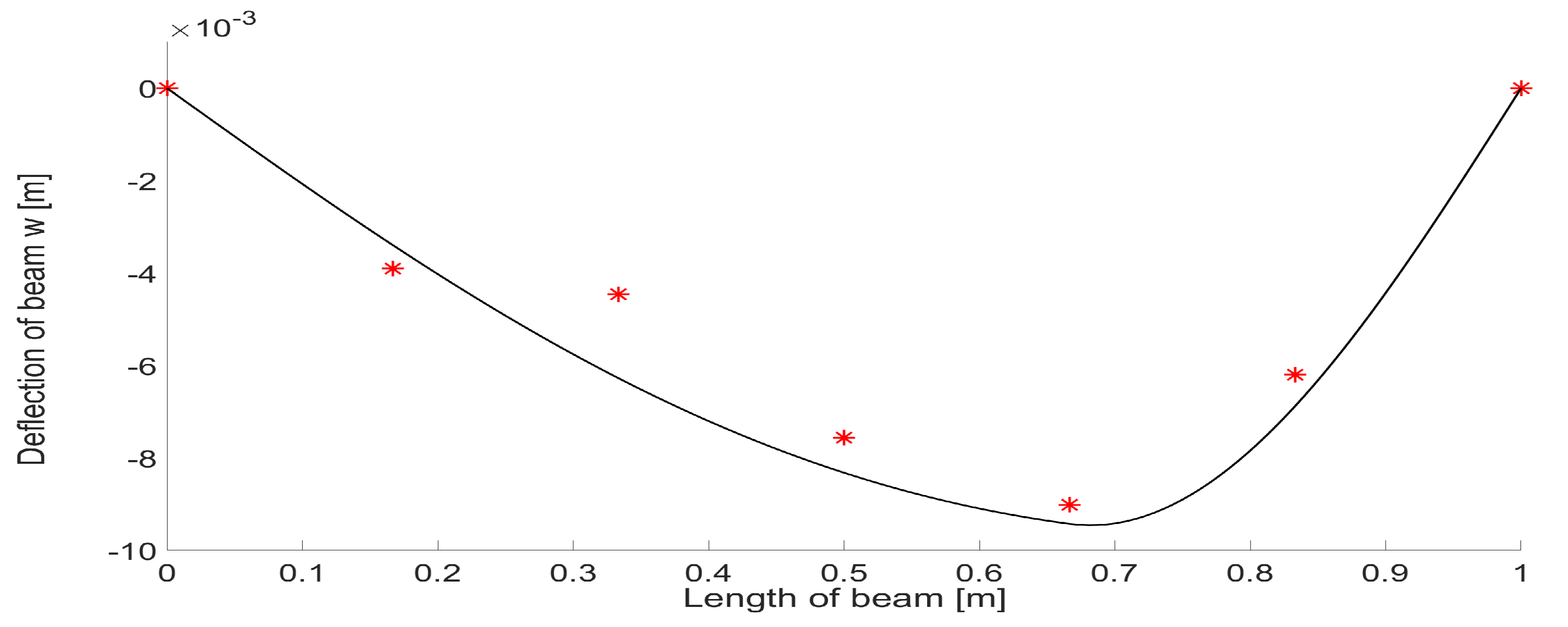The initial approximation is $\left((E_1^0,{\nu }_1^0),(E_2^0,{\nu }_2^0)\right)$—i.e., on the first interval $K_1$ is $(E_1^0,{\nu }_1^0)=(19\times {10}^{10},0.22)$ and on the second $K_2$ is $(E_2^0,{\nu }_2^0)=(27\times {10}^9,0.22).$ The numerical results are summarized in Table 1 where $it$ denotes the total number of iterations of the nonlinear conjugate gradient method. The deflection for computed material parameters $({\mathit{E}}^{\ast },{\mathit{\nu }}^{\ast })$ is shown in Figure 2 and Figure 3.

Table 1. Results of presented examples.

P	${\mathit{E}}^{\ast }$	${\mathit{\nu }}^{\ast }$	$\mathcal{J}\left(\mathbf{w}({\mathit{E}}^{\ast },{\mathit{\nu }}^{\ast })\right)$	$\mathit{i}\mathit{t}$
${10}^6$	${10}^{10}\times (20.9999,2.4999)$	$(0.1871,0.2412)$	$0.9914\times {10}^{-9}$	19
$-{10}^6$	${10}^{10}\times (20.9999,2.4618)$	$(0.1972,0.2482)$	$0.9892\times {10}^{-9}$	19

Figure 2. Deflection of the Gao beam for $P={10}^6$ N, $q=-4\times {10}^6{\mathrm{Nm}}^{-1}$ and $({\mathit{E}}^{\ast },{\mathit{\nu }}^{\ast })$. The asterisks stand for corresponding measured data $\mathbf{z}$ given in (46).

Figure 3. Deflection of the Gao beam for $P=-{10}^6$ N $q=-4\times {10}^6{\mathrm{Nm}}^{-1}$ and $({\mathit{E}}^{\ast },{\mathit{\nu }}^{\ast })$. The asterisks stand for corresponding measured data $\mathbf{z}$ given in (47).

Numerical computations were realized by Matlab.

7. Conclusions

In the theoretical part of the paper, we analyzed the identification problem for the Gao beam model. Firstly, the Gao beam equation was introduced. Further, the identification Young’s modulus and Poisson ratio, was formulated as an optimal control problem. Next, the existence theorem for simply supported beam was presented together with continuous dependence of the solution to the state problem on material parameters. Moreover, the discretization and convergence analysis of the studied identification problem was discussed. The theoretical results were completed by the numerical example.

Future research will be extended to more general cases, namely to an identification problem for the nonlinear Gao beam model supported by an elastic deformable foundation.