Upper Bounds and Explicit Formulas for the Ruin Probability in the Risk Model with Stochastic Premiums and a Multi-Layer Dividend Strategy

Abstract

This paper is devoted to the investigation of the ruin probability in the risk model with stochastic premiums where dividends are paid according to a multi-layer dividend strategy. We obtain an exponential bound for the ruin probability and investigate conditions, under which it holds for a number of distributions of the premium and claim sizes. Next, we use the exponential bound to construct non-exponential bounds for the ruin probability. We show that the non-exponential bounds turn out to be tighter than the exponential one in some cases. Moreover, we derive explicit formulas for the ruin probability when the premium and claim sizes have either the hyperexponential or the Erlang distributions and apply them to investigate how tight the bounds are. To illustrate and analyze the results obtained, we give numerical examples.

1. Introduction

One of the central objects investigated in risk theory is the ruin probability, which is the probability that the surplus of an insurance company becomes negative in some time interval and implies that the company is no longer able to reimburse claims. To calculate the ruin probability in different risk models, a great number of approaches has been proposed and studied recently (see the monographs [1,2,3,4,5,6] and references therein). Since Gerber and Shiu [7] introduced the expected discounted penalty function for the classical risk model, the ruin probability has often been investigated together with the surplus prior to ruin and the deficit at ruin in various risk models (see, e.g., [8,9,10,11,12,13,14] and references therein). The expected discounted penalty function, which is also called the Gerber–Shiu function, combines these three objects into one function, and the ruin probability is a special case of the function.

Risk models where the insurance company pays dividends to its shareholders have attracted great interest since De Finetti [15] considered dividend strategies for a binomial model. We mention only a few papers [16,17,18,19,20,21,22,23,24] devoted to the investigation of risk models with different dividend strategies. Multi-layer dividend strategies are of special interest because they enable to change the intensity of dividend payments depending on the current surplus. Different risk models with multi-layer dividend strategies are investigated in [25,26,27,28,29,30,31,32,33,34,35,36]. In particular, algorithmic schemes for the determination of explicit expressions for the Gerber–Shiu function and the expected discounted dividend payments in the classical risk model with multi-layer dividend strategies are developed in [25].

Although explicit formulas for the ruin probability are highly beneficial, it is well known that they can be obtained only in some special cases (see, e.g., [24,36,37,38,39,40,41,42,43], and also [44,45] for recursive formulas). That is why numerous bounds and approximations for the ruin probability are established and investigated in different risk models (see, e.g., [1,2,3,4,5] and references therein). Construction of exponential bounds is one of the key problems that is studied in risk theory (see, e.g., [46], [47] (Theorem 1), [48] (Theorem 1), [49] (Section 2), [50] (Theorem 2), [51] ([Theorem 5.1), [52] (Section 3), [53] (Theorems 2–4) and [54] (Theorem 2)). In particular, for the classical compound Poisson risk model, the exponential bound, which is also called the Lundberg inequality, can be derived in different ways (see, e.g., [1,2,3]), one of which is the martingale approach introduced by Gerber [46]. The supermartingale approach, which generalizes the martingale one and enables to construct exponential bounds in more complicated risk models, is applied in [4] (Chapters 7–9) and [51] (Sections 4 and 5). In some risk models, if claim sizes belong to heavy-tailed distributions, then the ruin probability decreases much more slowly compared with exponential rate with increasing initial surplus. Hence, exponential bounds do not hold any longer. Different non-exponential upper bounds for the ruin probability are obtained, e.g., in [48,55,56]. Moreover, a lot of papers are devoted to the construction of upper and lower bounds for the ruin probability in the compound Poisson risk model and its generalizations (see, e.g., [57,58,59,60,61]).

In this paper, we deal with the risk model considered in [36] where premiums are stochastic and dividends are paid according to a multi-layer dividend strategy. In what follows, we suppose that all stochastic objects are defined on a probability space $(\mathsf{\Omega },\mathfrak{F},\mathbb{P})$ satisfying the usual conditions. In the risk model considered in the present paper, premium sizes form a sequence ${\left\{{\widehat{Y}}_i\right\}}_{i⩾1}$ of non-negative independent and identically distributed (i.i.d.) random variables (r.v.s), which are independent copies of a r.v. $\widehat{Y}$ with cumulative distribution function (c.d.f.) $F_{\widehat{Y}}\left(y\right)=\mathbb{P}[\widehat{Y}⩽y]$, and the number of premiums on the time interval $[0,t]$ is a Poisson process ${\left\{{\widehat{N}}_t\right\}}_{t⩾0}$ with constant intensity $\widehat{\lambda }>0$. Similarly, claim sizes form a sequence ${\left\{Y_i\right\}}_{i⩾1}$ of i.i.d. r.v.s, which are independent copies of a r.v. Y with c.d.f. $F_Y\left(y\right)=\mathbb{P}[Y⩽y]$, and the number of claims on the time interval $[0,t]$ is a Poisson process ${\left\{N_t\right\}}_{t⩾0}$ with constant intensity $\lambda >0$. Thus, the total premiums and claims on $[0,t]$ equal ${\sum }_{i=1}^{{\widehat{N}}_t}{\widehat{Y}}_i$ and ${\sum }_{i=1}^{N_t}{Y}_i$, respectively. Here and subsequently, a sum is always set to be equal to 0 if the upper summation index is less than the lower one. Thus, ${\sum }_{i=1}^{{\widehat{N}}_t}{\widehat{Y}}_i=0$ if ${\widehat{N}}_t=0$, and ${\sum }_{i=1}^{N_t}{Y}_i=0$ if $N_t=0$. In what follows, we also assume that the r.v.s ${\left\{{\widehat{Y}}_i\right\}}_{i⩾1}$ and ${\left\{Y_i\right\}}_{i⩾1}$ have finite expectations $\widehat{\mu }>0$ and $\mu >0$, respectively, and ${\left\{{\widehat{Y}}_i\right\}}_{i⩾1}$, ${\left\{Y_i\right\}}_{i⩾1}$, ${\left\{{\widehat{N}}_t\right\}}_{t⩾0}$ and ${\left\{N_t\right\}}_{t⩾0}$ are mutually independent.

We denote a non-negative initial surplus by x, and let ${\left\{X_t\left(x\right)\right\}}_{t⩾0}$ be the surplus process provided that the initial surplus is x. Next, we make the additional assumption that dividends are paid to shareholders according to a k-layer dividend strategy with $k⩾1$. Let $\mathbf{b}=(b_0,\dots ,b_k)$ be a $(k+1)$-dimensional vector with real-valued components such that $0=b_0<b_1<\dots <b_{k-1}<b_k=\infty$. The k-layer dividend strategy $\mathbf{b}$ implies that dividends are paid continuously at a rate $d_j>0$ whenever $b_{j-1}⩽X_t\left(x\right)<b_j$, i.e., the process ${\left\{X_t\left(x\right)\right\}}_{t⩾0}$ is in the j-th layer at time t, where $1⩽j⩽k$. Then the surplus process ${\left\{X_t\left(x\right)\right\}}_{t⩾0}$ is defined by

$$X_t\left(x\right)=x+\sum _{i=1}^{{\widehat{N}}_t}{\widehat{Y}}_i-\sum _{i=1}^{N_t}{Y}_i-{\int }_0^t\sum _{j=1}^k{d}_j{\mathrm{𝟙}}_{\left\{b_{j-1}⩽X_s\left(x\right)<b_j\right\}}\mathrm{d}s,t⩾0,$$

(1)

where ${\mathrm{𝟙}}_{\{·\}}$ denotes the indicator function. Let $d_{\max }={max}_{1⩽j⩽k}\left\{d_j\right\}$. From now on, we suppose that the following net profit condition holds for the model described:

$$\widehat{\lambda }\widehat{\mu }>\lambda \mu +d_{\max }.$$

(2)

Next, let $\tau \left(x\right)=inf\{t⩾0:X_t\left(x\right)<0\}$ be the ruin time for the risk process ${\left\{X_t\left(x\right)\right\}}_{t⩾0}$ defined by (1). For $x⩾0$, the infinite-horizon ruin probability is defined by

$$\psi \left(x\right)=\mathbb{E}\left({\mathrm{𝟙}}_{\left\{\tau \right(x)<\infty \}}|X_0\left(x\right)=x\right).$$

As mentioned before, the ruin probability is a special case of the Gerber–Shiu function introduced in [7].

The model described above is investigated in [36] for $k⩾2$, where piecewise integro-differential equations for the Gerber–Shiu function and the expected discounted dividend payments until ruin are derived. Moreover, explicit formulas for the ruin probability as well as for the expected discounted dividend payments are obtained in [36] in the case of exponentially distributed claim and premium sizes. The special case of this model where $k=1$ is studied in [62]. In that paper, five-moment and three-moment analogues to the De Vylder approximation for the ruin probability are constructed, the accuracy of those approximations is analyzed and an explicit formula for the ruin probability in the case of exponentially distributed premium and claim sizes is obtained. Furthermore, the risk model with stochastic premiums and some its modifications are investigated in [24,47,63,64,65,66,67,68,69,70,71,72] (see also [3] (Chapters XI and XII), [4] (Chapters 1, 3 and 6) and references therein).

The aim of the present paper was to construct upper exponential and non-exponential bounds for the ruin probability in the model described above as well as to obtain explicit formulas for it and analyze the results in detail for the exponential, hyperexponential and Erlang distributions of the premium and claim sizes. To get the exponential bound, we reduce our model to the model with a constant dividend strategy, to which we apply the martingale approach introduced by Gerber [46]. To improve our exponential bound, i.e., to obtain tighter bounds, we construct non-exponential bounds using the exponential bound. We deal with light-tailed distributions of claim sizes, and the existence of their finite exponential moments is necessary for the construction of our non-exponential bounds. Thus, in contrast to other papers where non-exponential bounds are usually obtained when exponential bounds do not exist (see, e.g., [48,55,56,57,58,59,60,61]), our non-exponential bounds are based on the exponential one and proved to be tighter in some cases, especially for relatively small values of the initial surplus. To analyze the accuracy of the bounds, we derive explicit formulas for the ruin probability when the premium and claim sizes have either the hyperexponential or the Erlang distributions as well as apply explicit formulas obtained in [36,62] in the case of exponentially distributed premium and claim sizes. Note that although the exponential case is investigated in detail in [36,62] and explicit formulas are available, it is still worth being considered for the following two reasons: firstly, the bounds seem to be more elegant and easier to apply than the explicit formulas, especially when their accuracy is acceptable or the number of layers is large, and secondly, it is the only case where the explicit formulas are not so complicated and can be used to analyze the accuracy of the bounds if the number of layers is more than one.

The rest of the paper is organized as follows. In Section 2, we formulate two theorems, which follow immediately from results obtained in [36,62] and are often referred to in our main results. In Section 3, we get an exponential bound for the ruin probability and investigate conditions, under which it holds for a number of distributions of the premium and claim sizes. In Section 4, we obtain non-exponential bounds for the ruin probability using the exponential bound and show that they turn out to be tighter than the exponential one in some cases. These non-exponential bounds, which are given in Theorems 7 and 8, are the main result of the paper. Section 5 is devoted to the construction of explicit formulas for the ruin probability when the premium and claim sizes have either the hyperexponential or the Erlang distributions. Numerical illustrations are given in Section 6, where, in particular, the explicit formulas obtained in Section 5 and [36,62] are applied in order to investigate how tight the exponential and non-exponential bounds are.

2. Preliminary Results

We now formulate some auxiliary results, which are frequently used in the rest of the paper. Theorem 1 below is a special case of Theorem 1 in [36], which is formulated for the Gerber–Shiu function in the model where $k⩾2$. The assertion of the theorem is given in [62] for the case $k=1$.

Theorem 1. 

Let the surplus process ${\left\{X_t\left(x\right)\right\}}_{t⩾0}$ be defined by (1) under the above assumptions, and let $F_Y\left(y\right)$ be continuous on ${\mathbb{R}}_{+}$. Then the function $\psi \left(x\right)$ is differentiable on the intervals $[b_{j-1},b_j]$ for all $1⩽j⩽k$ and satisfies the piecewise integro-differential equation

$$\begin{array}{cc}\hfill & d_j{\psi }^{\prime }\left(x\right)+(\lambda +\widehat{\lambda })\psi \left(x\right)=\widehat{\lambda }{\int }_0^{\infty }\psi (x+y)\mathrm{d}{F}_{\widehat{Y}}\left(y\right)\hfill \\ \hfill & +\lambda {\int }_0^x\psi (x-y)\mathrm{d}{F}_Y\left(y\right)+\lambda \left(1-F_Y\left(x\right)\right),x\in [b_{j-1},b_j].\hfill \end{array}$$

(3)

Note that here the derivatives of $\psi \left(x\right)$ at the ends of the closed intervals $[b_{j-1},b_j]$ are assumed to be one-sided. Moreover, although we imply the interval $[b_{k-1},\infty )$ instead of $[b_{j-1},b_j]$ if $j=k$, for the sake of convenience and compactness, we do write $[b_{j-1},b_j]$ for all $1⩽j⩽k$.

Remark 1. 

To solve Equation (3), we use the following natural boundary conditions (see [36,62]). The first $k-1$ conditions are easily obtained from the equality ${\psi }_j\left(b_j\right)={\psi }_{j+1}\left(b_j\right)$ for all $1⩽j⩽k-1$. Next, using the standard considerations (see, e.g., [2] (pp. 153, 162), [4] (Lemma 1.1) or [42] (Lemma 2.1)) it can be shown easily that ${lim}_{x\to \infty }\psi \left(x\right)=0$ provided that the net profit condition (2) holds. Finally, it is obvious that $\psi \left(0\right)=1$ for this risk model.

Now we fix $j\in \{1,2,\dots ,k\}$ and define the following functions for all $x\in [b_{j-1},b_j]$:

$$a_1\left(x\right)=(x-b_{j-1})/d_j+(b_{j-1}-b_{j-2})/d_{j-1}+\dots +(b_2-b_1)/d_2+(b_1-b_0)/d_1,$$

$$a_2\left(x\right)=(x-b_{j-1})/d_j+(b_{j-1}-b_{j-2})/d_{j-1}+\dots +(b_2-b_1)/d_2,$$

$$\dots$$

$$a_{j-1}\left(x\right)=(x-b_{j-1})/d_j+(b_{j-1}-b_{j-2})/d_{j-1},$$

$$a_j\left(x\right)=(x-b_{j-1})/d_j.$$

The next assertion follows immediately from the proof of Theorem 1 in [36].

Theorem 2. 

Let the surplus process ${\left\{X_t\left(x\right)\right\}}_{t⩾0}$ be defined by (1) under the above assumptions. Then for any $1⩽j⩽k$, we have

$$\psi \left(x\right)=I_j\left(x\right)+I_{j-1}\left(x\right)+\dots +I_1\left(x\right)+I_0\left(x\right),x\in [b_{j-1},b_j],$$

(4)

where

$$\begin{array}{cc}\hfill I_j\left(x\right)& =\frac{1}{d_j}{e}^{-(\lambda +\widehat{\lambda })x/d_j}{\int }_{b_{j-1}}^x{e}^{(\lambda +\widehat{\lambda })s/d_j}(\widehat{\lambda }{\int }_0^{\infty }\psi (s+y)\mathrm{d}{F}_{\widehat{Y}}\left(y\right)\hfill \\ \hfill & +\lambda {\int }_0^s\psi (s-y)\mathrm{d}{F}_Y\left(y\right)+\lambda \left(1-F_Y\left(s\right)\right))\mathrm{d}s,\hfill \end{array}$$

$$\begin{array}{cc}\hfill I_{j-1}\left(x\right)& =\frac{1}{d_{j-1}}{e}^{-(\lambda +\widehat{\lambda })(a_j\left(x\right)+b_{j-1}/d_{j-1})}{\int }_{b_{j-2}}^{b_{j-1}}{e}^{(\lambda +\widehat{\lambda })s/d_{j-1}}(\widehat{\lambda }{\int }_0^{\infty }\psi (s+y)\mathrm{d}{F}_{\widehat{Y}}\left(y\right)\hfill \\ \hfill & +\lambda {\int }_0^s\psi (s-y)\mathrm{d}{F}_Y\left(y\right)+\lambda \left(1-F_Y\left(s\right)\right))\mathrm{d}s,\hfill \end{array}$$

$$\dots$$

$$\begin{array}{cc}\hfill I_1\left(x\right)& =\frac{1}{d_1}{e}^{-(\lambda +\widehat{\lambda })(a_2\left(x\right)+b_1/d_1)}{\int }_{b_0}^{b_1}{e}^{(\lambda +\widehat{\lambda })s/d_1}(\widehat{\lambda }{\int }_0^{\infty }\psi (s+y)\mathrm{d}{F}_{\widehat{Y}}\left(y\right)\hfill \\ \hfill & +\lambda {\int }_0^s\psi (s-y)\mathrm{d}{F}_Y\left(y\right)+\lambda \left(1-F_Y\left(s\right)\right))\mathrm{d}s,\hfill \end{array}$$

$$I_0\left(x\right)=e^{-(\lambda +\widehat{\lambda })a_1\left(x\right)}.$$

Note that a simple lower bound for $\psi \left(x\right)$ follows immediately from the assertion of Theorem 2. To be more precise, for any $1⩽j⩽k$, we have $\psi \left(x\right)⩾e^{-(\lambda +\widehat{\lambda })a_1\left(x\right)}$, $x\in [b_{j-1},b_j]$. This bound is not so tight and can be improved. Nonetheless, in what follows, we concentrate on the construction of upper bounds for $\psi \left(x\right)$.

3. Exponential Bound for the Ruin Probability

In this section, we obtain an exponential bound for the ruin probability and we investigate conditions, under which it holds for a number of distributions of the premium and claim sizes.

3.1. Exponential Bound

Consider the surplus process ${\left\{{\tilde{X}}_t\left(x\right)\right\}}_{t⩾0}$ defined by

$${\tilde{X}}_t\left(x\right)=x+\sum _{i=1}^{{\widehat{N}}_t}{\widehat{Y}}_i-\sum _{i=1}^{N_t}{Y}_i-d_{\max }t,t⩾0.$$

(5)

Let $\tilde{\tau }\left(x\right)=inf\{t⩾0:{\tilde{X}}_t\left(x\right)<0\}$ and $\tilde{\psi }\left(x\right)=\mathbb{E}\left[\mathrm{𝟙}(\tilde{\tau }\left(x\right)<\infty )\right|{\tilde{X}}_0\left(x\right)=x]$ be the ruin time and the infinite-horizon ruin probability for ${\left({\tilde{X}}_t\left(x\right)\right)}_{t⩾0}$.

Lemma 1. 

Let ${\left\{{\tilde{X}}_t\left(x\right)\right\}}_{t⩾0}$ be the surplus process defined by Equation (5) under the above assumptions. If there exists $R>0$ such that

$$\widehat{\lambda }\left(\mathbb{E}\left[e^{-R\widehat{Y}}\right]-1\right)+\lambda \left(\mathbb{E}\left[e^{RY}\right]-1\right)+d_{\max }R=0,$$

(6)

then

$$\tilde{\psi }\left(x\right)⩽e^{-Rx}forallx⩾0.$$

The proof of Lemma 1 is similar to the proof of Theorem 1.8 together with Lemma 1.3 in [4] (see also [1] (pp. 10–11), [47] (Theorem 1) or [50] (Theorem 2 together with Lemma 1)) and is based on the martingale approach introduced by Gerber [46]. The main idea is to show that if there exists $R>0$ such that (6) holds, then the exponential process ${\left\{exp\left(-R\left({\sum }_{i=1}^{{\widehat{N}}_t}{\widehat{Y}}_i-{\sum }_{i=1}^{N_t}{Y}_i-d_{\max }t\right)\right)\right\}}_{t⩾0}$ is a martingale w.r.t. the filtration generated by ${\left\{{\widehat{Y}}_i\right\}}_{i⩾1}$, ${\left\{Y_i\right\}}_{i⩾1}$, ${\left\{{\widehat{N}}_t\right\}}_{t⩾0}$ and ${\left\{N_t\right\}}_{t⩾0}$, and then to apply the optional stopping theorem.

Theorem 3. 

Let the surplus process ${\left\{X_t\left(x\right)\right\}}_{t⩾0}$ be defined by (1) under the above assumptions. If there is $R>0$ such that (6) holds, then, for all $x⩾0$,

$$\psi \left(x\right)⩽e^{-Rx}.$$

(7)

The proof of Theorem 3 follows immediately from Lemma 1. Indeed, since ${\tilde{X}}_t\left(x\right)⩽X_t\left(x\right)$ a.s. for all $t⩾0$ and $x⩾0$, we conclude that $\tilde{\tau }\left(x\right)⩽\tau \left(x\right)$ a.s. and, consequently, $\psi \left(x\right)⩽\tilde{\psi }\left(x\right)$ for all $x⩾0$.

Hence, the exponential estimate of ruin probability ${\psi }_{\exp }\left(x\right)=e^{-Rx}$ holds for all $x⩾0$.

3.2. Exponential Distributions for the Premium and Claim Sizes

We now suppose that the premium and claim sizes are exponentially distributed, i.e., their probability density functions (p.d.f.s) are $f_{\widehat{Y}}\left(y\right)=e^{-y/\widehat{\mu }}/\widehat{\mu }$ and $f_Y\left(y\right)=e^{-y/\mu }/\mu$, $y⩾0$, respectively.

Theorem 4. 

Let the surplus process ${\left\{X_t\left(x\right)\right\}}_{t⩾0}$ be defined by (1) under the above assumptions, and let the premium and claim sizes be exponentially distributed with means $\widehat{\mu }$ and μ, respectively. Then condition (6) holds with

$$R=\frac{\mu \widehat{\mu }(\lambda +\widehat{\lambda })+d_{\max }(\widehat{\mu }-\mu )-\sqrt{{\left(\mu \widehat{\mu }(\lambda +\widehat{\lambda })+d_{\max }(\widehat{\mu }-\mu )\right)}^2-4d_{\max }\mu \widehat{\mu }\left(\widehat{\lambda }\widehat{\mu }-\lambda \mu -d_{\max }\right)}}{2d_{\max }\mu \widehat{\mu }}$$

(8)

if and only if the net profit condition (2) is true.

Proof. 

Since

$$\mathbb{E}\left[e^{-R\widehat{Y}}\right]=\frac{1}{1+\widehat{\mu }R},R⩾0,\mathrm{and}\mathbb{E}\left[e^{RY}\right]=\frac{1}{1-\mu R},0⩽R<\frac{1}{\mu },$$

condition (6) takes the form

$$\widehat{\lambda }\left(\frac{1}{1+\widehat{\mu }R}-1\right)+\lambda \left(\frac{1}{1-\mu R}-1\right)+d_{\max }R=0,0<R<\frac{1}{\mu },$$

from which we get either $R=0$, which does not meet the condition $0<R<1/\mu$, or

$$d_{\max }\mu \widehat{\mu }{R}^2-\left(\mu \widehat{\mu }(\lambda +\widehat{\lambda })+d_{\max }(\widehat{\mu }-\mu )\right)R+\widehat{\lambda }\widehat{\mu }-\lambda \mu -d_{\max }=0.$$

(9)

Note that the discriminant of (9) is always positive. Indeed, we have

$$\begin{array}{cc}\hfill & {\left(\mu \widehat{\mu }(\lambda +\widehat{\lambda })+d_{\max }(\widehat{\mu }-\mu )\right)}^2-4d_{\max }\mu \widehat{\mu }\left(\widehat{\lambda }\widehat{\mu }-\lambda \mu -d_{\max }\right)\hfill \\ \hfill & ={\left(\mu \widehat{\mu }(\widehat{\lambda }-\lambda )-d_{\max }(\mu +\widehat{\mu })\right)}^2+4\lambda \widehat{\lambda }{\left(\mu \widehat{\mu }\right)}^2>0.\hfill \end{array}$$

Hence, (9) has two real roots:

$$R_{1,2}=\frac{\mu \widehat{\mu }(\lambda +\widehat{\lambda })+d_{\max }(\widehat{\mu }-\mu )\pm \sqrt{{\left(\mu \widehat{\mu }(\lambda +\widehat{\lambda })+d_{\max }(\widehat{\mu }-\mu )\right)}^2-4d_{\max }\mu \widehat{\mu }\left(\widehat{\lambda }\widehat{\mu }-\lambda \mu -d_{\max }\right)}}{2d_{\max }\mu \widehat{\mu }}.$$

For definiteness, we assume that $R_1<R_2$. We now show that $R_1<1/\mu$ and $R_2>1/\mu$.

Indeed, $R_1<1/\mu$ if and only if

$$\mu \widehat{\mu }(\lambda +\widehat{\lambda })+d_{\max }(\widehat{\mu }-\mu )-\sqrt{{\left(\mu \widehat{\mu }(\lambda +\widehat{\lambda })+d_{\max }(\widehat{\mu }-\mu )\right)}^2-4d_{\max }\mu \widehat{\mu }\left(\widehat{\lambda }\widehat{\mu }-\lambda \mu -d_{\max }\right)}<2d_{\max }\widehat{\mu }$$

or, equivalently,

$$\mu \widehat{\mu }(\lambda +\widehat{\lambda })-d_{\max }(\mu +\widehat{\mu })<\sqrt{{\left(\mu \widehat{\mu }(\lambda +\widehat{\lambda })+d_{\max }(\widehat{\mu }-\mu )\right)}^2-4d_{\max }\mu \widehat{\mu }\left(\widehat{\lambda }\widehat{\mu }-\lambda \mu -d_{\max }\right)}.$$

(10)

To prove that (10) is true, it is enough to show that

$${\left(\mu \widehat{\mu }(\lambda +\widehat{\lambda })-d_{\max }(\mu +\widehat{\mu })\right)}^2-{\left(\mu \widehat{\mu }(\lambda +\widehat{\lambda })+d_{\max }(\widehat{\mu }-\mu )\right)}^2<-4d_{\max }\mu \widehat{\mu }\left(\widehat{\lambda }\widehat{\mu }-\lambda \mu -d_{\max }\right).$$

(11)

Simplifying (11) yields $\widehat{\mu }>-\mu$, which is always true. Thus, $R_1<1/\mu$. Similarly, $R_2>1/\mu$ if and only if

$$\mu \widehat{\mu }(\lambda +\widehat{\lambda })+d_{\max }(\widehat{\mu }-\mu )+\sqrt{{\left(\mu \widehat{\mu }(\lambda +\widehat{\lambda })+d_{\max }(\widehat{\mu }-\mu )\right)}^2-4d_{\max }\mu \widehat{\mu }\left(\widehat{\lambda }\widehat{\mu }-\lambda \mu -d_{\max }\right)}>2d_{\max }\widehat{\mu }$$

or, equivalently,

$$\sqrt{{\left(\mu \widehat{\mu }(\lambda +\widehat{\lambda })+d_{\max }(\widehat{\mu }-\mu )\right)}^2-4d_{\max }\mu \widehat{\mu }\left(\widehat{\lambda }\widehat{\mu }-\lambda \mu -d_{\max }\right)}>d_{\max }(\mu +\widehat{\mu })-\mu \widehat{\mu }(\lambda +\widehat{\lambda }).$$

(12)

To prove (12), it is enough to show that

$${\left(\mu \widehat{\mu }(\lambda +\widehat{\lambda })+d_{\max }(\widehat{\mu }-\mu )\right)}^2-{\left(d_{\max }(\mu +\widehat{\mu })-\mu \widehat{\mu }(\lambda +\widehat{\lambda })\right)}^2>4d_{\max }\mu \widehat{\mu }\left(\widehat{\lambda }\widehat{\mu }-\lambda \mu -d_{\max }\right),$$

which is equivalent to (11) and, consequently, always true. Therefore, $R_2>1/\mu$.

Next, if the net profit condition (2) holds, then by Vieta’s theorem, both roots of (9) have the same sign. Since $R_2>1/\mu$, we conclude that $R_1>0$. Thus, condition (6) holds with R given by (8).

If the net profit condition (2) does not hold, i.e., $\widehat{\lambda }\widehat{\mu }-\lambda \mu -d_{\max }⩽0$, then by Vieta’s theorem, $R_1⩽0$ and $R_2>1/\mu$. Hence, there is no R from the interval $(0,1/\mu )$, which completes the proof. □

3.3. Hyperexponential Distributions for the Premium and Claim Sizes

Now let

$$F_{\widehat{Y}}\left(y\right)={\widehat{p}}_1{F}_{\widehat{Y},1}\left(y\right)+{\widehat{p}}_2{F}_{\widehat{Y},2}\left(y\right)+\dots +{\widehat{p}}_{\widehat{n}}{F}_{\widehat{Y},\widehat{n}}\left(y\right),y⩾0,$$

where $\widehat{n}⩾1$, ${\widehat{p}}_i>0$, $F_{\widehat{Y},i}$ is the c.d.f. of the exponential distribution with mean ${\widehat{\mu }}_i>0$ for all $1⩽i⩽\widehat{k}$, all ${\widehat{\mu }}_i$ are distinct, ${\sum }_{i=1}^{\widehat{n}}{\widehat{p}}_i=1$ and ${\sum }_{i=1}^{\widehat{n}}{\widehat{p}}_i{\widehat{\mu }}_i=\widehat{\mu }$. In addition, let

$$F_Y\left(y\right)=p_1{F}_{Y,1}\left(y\right)+p_2{F}_{Y,2}\left(y\right)+\dots +p_n{F}_{Y,n}\left(y\right),y⩾0,$$

where $n⩾1$, $p_i>0$, $F_{Y,i}$ is the c.d.f. of the exponential distribution with mean ${\mu }_i>0$ for all $1⩽i⩽n$, all ${\mu }_i$ are distinct, ${\sum }_{i=1}^n{p}_i=1$ and ${\sum }_{i=1}^n{p}_i{\mu }_i=\mu$. We set ${\mu }_{\max }={max}_{1⩽i⩽n}\left\{{\mu }_i\right\}$.

Theorem 5. 

Let the surplus process ${\left\{X_t\left(x\right)\right\}}_{t⩾0}$ be defined by (1) under the above assumptions, and let the premium and claim sizes have the hyperexponential distributions described at the beginning of this section above. Then the condition (6) holds with R defined as a root of the equation

$$\begin{array}{cc}\hfill & -\widehat{\lambda }\left(\prod _{i=1}^n(1-{\mu }_{i}R)\right)\sum _{i=1}^{\widehat{n}}\left({\widehat{p}}_i{\widehat{\mu }}_i\prod _{\begin{array}{c}l=1\\ l\ne i\end{array}}^{\widehat{n}}(1+{\widehat{\mu }}_{i}R)\right)+\lambda \left(\prod _{i=1}^{\widehat{n}}(1+{\widehat{\mu }}_{i}R)\right)\sum _{i=1}^n\left(p_i{\mu }_i\prod _{\begin{array}{c}l=1\\ l\ne i\end{array}}^n(1-{\mu }_{i}R)\right)\hfill \\ \hfill & +d_{\max }\left(\prod _{i=1}^{\widehat{n}}(1+{\widehat{\mu }}_{i}R)\right)\left(\prod _{i=1}^n(1-{\mu }_{i}R)\right)=0\hfill \end{array}$$

(13)

belonging to the interval $(0,1/{\mu }_{\max })$, which exists provided that the net profit condition (2) is satisfied.

Proof. 

Let m be the value of i in ${\mu }_{\max }={max}_{1⩽i⩽n}\left\{{\mu }_i\right\}$ such that ${\mu }_m={\mu }_{\max }$. It can be easily checked that

$$\mathbb{E}\left[e^{-R\widehat{Y}}\right]=\sum _{i=1}^{\widehat{n}}\frac{{\widehat{p}}_i}{1+{\widehat{\mu }}_{i}R},R⩾0,\mathrm{and}\mathbb{E}\left[e^{RY}\right]=\sum _{i=1}^n\frac{p_i}{1-{\mu }_{i}R},0⩽R<\frac{1}{{\mu }_{\max }}.$$

Therefore, condition (6) takes the form

$$\widehat{\lambda }\left(\sum _{i=1}^{\widehat{n}}\frac{{\widehat{p}}_i}{1+{\widehat{\mu }}_{i}R}-1\right)+\lambda \left(\sum _{i=1}^n\frac{p_i}{1-{\mu }_{i}R}-1\right)+d_{\max }R=0,0<R<\frac{1}{{\mu }_{\max }}.$$

(14)

Multiplying (14) by $\left({\prod }_{i=1}^{\widehat{n}}(1+{\widehat{\mu }}_{i}R)\right)\left({\prod }_{i=1}^n(1-{\mu }_{i}R)\right)$ yields

$$\begin{array}{cc}\hfill & \widehat{\lambda }\left(\prod _{i=1}^n(1-{\mu }_{i}R)\right)\left(\sum _{i=1}^{\widehat{n}}\left({\widehat{p}}_i\prod _{\begin{array}{c}l=1\\ l\ne i\end{array}}^{\widehat{n}}(1+{\widehat{\mu }}_{i}R)\right)-\prod _{i=1}^{\widehat{n}}(1+{\widehat{\mu }}_{i}R)\right)\hfill \\ \hfill & +\lambda \left(\prod _{i=1}^{\widehat{n}}(1+{\widehat{\mu }}_{i}R)\right)\left(\sum _{i=1}^n\left(p_i\prod _{\begin{array}{c}l=1\\ l\ne i\end{array}}^n(1-{\mu }_{i}R)\right)-\prod _{i=1}^n(1-{\mu }_{i}R)\right)\hfill \\ \hfill & +d_{\max }R\left(\prod _{i=1}^{\widehat{n}}(1+{\widehat{\mu }}_{i}R)\right)\left(\prod _{i=1}^n(1-{\mu }_{i}R)\right)=0.\hfill \end{array}$$

(15)

Taking into account that

$$\begin{array}{cc}\hfill & \sum _{i=1}^{\widehat{n}}\left({\widehat{p}}_i\prod _{\begin{array}{c}l=1\\ l\ne i\end{array}}^{\widehat{n}}(1+{\widehat{\mu }}_{i}R)\right)-\prod _{i=1}^{\widehat{n}}(1+{\widehat{\mu }}_{i}R)=\sum _{i=1}^{\widehat{n}}{\widehat{p}}_i\left(\prod _{\begin{array}{c}l=1\\ l\ne i\end{array}}^{\widehat{n}}(1+{\widehat{\mu }}_{i}R)-\prod _{i=1}^{\widehat{n}}(1+{\widehat{\mu }}_{i}R)\right)\hfill \\ \hfill & =\sum _{i=1}^{\widehat{n}}\left({\widehat{p}}_i(-{\widehat{\mu }}_{i}R)\prod _{\begin{array}{c}l=1\\ l\ne i\end{array}}^{\widehat{n}}(1+{\widehat{\mu }}_{i}R)\right)\hfill \end{array}$$

and

$$\begin{array}{cc}\hfill & \sum _{i=1}^n\left(p_i\prod _{\begin{array}{c}l=1\\ l\ne i\end{array}}^n(1-{\mu }_{i}R)\right)-\prod _{i=1}^n(1-{\mu }_{i}R)=\sum _{i=1}^n{p}_i\left(\prod _{\begin{array}{c}l=1\\ l\ne i\end{array}}^n(1-{\mu }_{i}R)-\prod _{i=1}^n(1-{\mu }_{i}R)\right)\hfill \\ \hfill & =\sum _{i=1}^n\left(p_i\left({\mu }_{i}R\right)\prod _{\begin{array}{c}l=1\\ l\ne i\end{array}}^n(1-{\mu }_{i}R)\right),\hfill \end{array}$$

from (15) we get

$$\begin{array}{cc}\hfill & -\widehat{\lambda }\left(\prod _{i=1}^n(1-{\mu }_{i}R)\right)\sum _{i=1}^{\widehat{n}}\left({\widehat{p}}_i{\widehat{\mu }}_{i}R\prod _{\begin{array}{c}l=1\\ l\ne i\end{array}}^{\widehat{n}}(1+{\widehat{\mu }}_{i}R)\right)+\lambda \left(\prod _{i=1}^{\widehat{n}}(1+{\widehat{\mu }}_{i}R)\right)\sum _{i=1}^n\left(p_i{\mu }_{i}R\prod _{\begin{array}{c}l=1\\ l\ne i\end{array}}^n(1-{\mu }_{i}R)\right)\hfill \\ \hfill & +d_{\max }R\left(\prod _{i=1}^{\widehat{n}}(1+{\widehat{\mu }}_{i}R)\right)\left(\prod _{i=1}^n(1-{\mu }_{i}R)\right)=0.\hfill \end{array}$$

(16)

Since we are looking for $R\in (0,1/{\mu }_{\max })$, we can divide (16) by R, which gives (13).

Now we show that (13) has at least one root on interval $(0,1/{\mu }_{\max })$. To this end, we define the function $h\left(R\right)$ on $[0,1/{\mu }_{\max }]$ as follows:

$$\begin{array}{cc}\hfill h\left(R\right)& =-\widehat{\lambda }\left(\prod _{i=1}^n(1-{\mu }_{i}R)\right)\sum _{i=1}^{\widehat{n}}\left({\widehat{p}}_i{\widehat{\mu }}_i\prod _{\begin{array}{c}l=1\\ l\ne i\end{array}}^{\widehat{n}}(1+{\widehat{\mu }}_{i}R)\right)+\lambda \left(\prod _{i=1}^{\widehat{n}}(1+{\widehat{\mu }}_{i}R)\right)\sum _{i=1}^n\left(p_i{\mu }_i\prod _{\begin{array}{c}l=1\\ l\ne i\end{array}}^n(1-{\mu }_{i}R)\right)\hfill \\ \hfill & +d_{\max }\left(\prod _{i=1}^{\widehat{n}}(1+{\widehat{\mu }}_{i}R)\right)\left(\prod _{i=1}^n(1-{\mu }_{i}R)\right).\hfill \end{array}$$

It is easily seen that

$$h\left(0\right)=-\widehat{\lambda }\widehat{\mu }+\lambda \mu +d_{\max },$$

which is negative provided that the net profit condition (2) holds, and

$$h\left(\frac{1}{{\mu }_{\max }}\right)=\lambda \prod _{i=1}^{\widehat{n}}\left(1+\frac{{\widehat{\mu }}_i}{{\mu }_{\max }}\right)·p_m{\mu }_{\max }\prod _{\begin{array}{c}l=1\\ l\ne m\end{array}}^n\left(1-\frac{{\mu }_l}{{\mu }_{\max }}\right)>0.$$

Therefore, since $h\left(R\right)$ is continuous on $[0,1/{\mu }_{\max }]$, there is $R\in (0,1/{\mu }_{\max })$ such that $h\left(R\right)=0$, i.e., (13) has at least one root in the interval $(0,1/{\mu }_{\max })$. □

3.4. Erlang Distributions for the Premium and Claim Sizes

Now let the p.d.f.s of $\widehat{Y}$ and Y be

$$f_{\widehat{Y}}\left(y\right)=\frac{1}{(\widehat{n}-1)!{\widehat{\beta }}^{\widehat{n}}}{y}^{\widehat{n}-1}{e}^{-y/\widehat{\beta }},f_Y\left(y\right)=\frac{1}{(n-1)!{\beta }^n}{y}^{n-1}{e}^{-y/\beta },y⩾0,$$

where $\widehat{n}\in \mathbb{N}$, $n\in \mathbb{N}$, $\widehat{\beta }>0$, $\beta >0$, $\widehat{n}\widehat{\beta }=\widehat{\mu }$ and $n\beta =\mu$.

Theorem 6. 

Let the surplus process ${\left\{X_t\left(x\right)\right\}}_{t⩾0}$ be defined by (1) under the above assumptions, and let the premium and claim sizes have the Erlang distributions described above. Then the condition (6) holds with R defined as a root of the equation

$$\begin{array}{cc}\hfill & d_{\max }{(1+\widehat{\beta }R)}^{\widehat{n}}{(1-\beta R)}^n+\lambda \beta {(1+\widehat{\beta }R)}^{\widehat{n}}\sum _{i=1}^n\left(\genfrac{}{}{0pt}{}{n}{i}\right){(-\beta R)}^{i-1}\hfill \\ \hfill & -\widehat{\lambda }\widehat{\beta }{(1-\beta R)}^n\sum _{i=1}^{\widehat{n}}\left(\genfrac{}{}{0pt}{}{\widehat{n}}{i}\right){\left(\widehat{\beta }R\right)}^{i-1}=0\hfill \end{array}$$

(17)

on the interval $(0,1/\beta )$, which exists under the net profit condition (2).

Note that here and everywhere, symbols $\left(\genfrac{}{}{0pt}{}{n}{i}\right)$ and $\left(\genfrac{}{}{0pt}{}{\widehat{n}}{i}\right)$ denote binomial coefficients.

Proof. 

A standard computation shows that

$$\mathbb{E}\left[e^{-R\widehat{Y}}\right]={\left(\frac{1}{1+\widehat{\beta }R}\right)}^{\widehat{n}},R⩾0,\mathrm{and}\mathbb{E}\left[e^{RY}\right]={\left(\frac{1}{1-\beta R}\right)}^n,0⩽R<\frac{1}{\beta }.$$

Therefore, condition (6) takes the form

$$\widehat{\lambda }\left({\left(\frac{1}{1+\widehat{\beta }R}\right)}^{\widehat{n}}-1\right)+\lambda \left({\left(\frac{1}{1-\beta R}\right)}^n-1\right)+d_{\max }R=0,0<R<\frac{1}{\beta }.$$

(18)

Multiplying (18) by ${(1+\widehat{\beta }R)}^{\widehat{n}}{(1-\beta R)}^n$ gives

$$\widehat{\lambda }{(1-\beta R)}^n+\lambda {(1+\widehat{\beta }R)}^{\widehat{n}}+(d_{\max }R-\lambda -\widehat{\lambda }){(1+\widehat{\beta }R)}^{\widehat{n}}{(1-\beta R)}^n=0.$$

(19)

Since ${(1-\beta R)}^n={\sum }_{i=0}^n\left(\genfrac{}{}{0pt}{}{n}{i}\right){(-\beta R)}^i$ and ${(1+\widehat{\beta }R)}^{\widehat{n}}={\sum }_{i=0}^{\widehat{n}}\left(\genfrac{}{}{0pt}{}{\widehat{n}}{i}\right){\left(\widehat{\beta }R\right)}^i$, from (19) we obtain

$$\begin{array}{cc}& \widehat{\lambda }\sum _{i=1}^n\left(\genfrac{}{}{0pt}{}{n}{i}\right){(-\beta R)}^i+\lambda \sum _{i=1}^{\widehat{n}}\left(\genfrac{}{}{0pt}{}{\widehat{n}}{i}\right){\left(\widehat{\beta }R\right)}^i+d_{\max }R{(1+\widehat{\beta }R)}^{\widehat{n}}{(1-\beta R)}^n\hfill \\ & -(\lambda +\widehat{\lambda })\left(\sum _{i=1}^n\left(\genfrac{}{}{0pt}{}{n}{i}\right){(-\beta R)}^i+\sum _{i=1}^{\widehat{n}}\left(\genfrac{}{}{0pt}{}{\widehat{n}}{i}\right){\left(\widehat{\beta }R\right)}^i+\left(\sum _{i=1}^n\left(\genfrac{}{}{0pt}{}{n}{i}\right){(-\beta R)}^i\right)\left(\sum _{i=1}^{\widehat{n}}\left(\genfrac{}{}{0pt}{}{\widehat{n}}{i}\right){\left(\widehat{\beta }R\right)}^i\right)\right)=0.\hfill \end{array}$$

(20)

Dividing (20) by R and rearranging the terms we get

$$\begin{array}{cc}\hfill & d_{\max }{(1+\widehat{\beta }R)}^{\widehat{n}}{(1-\beta R)}^n+\lambda \beta \sum _{i=1}^n\left(\genfrac{}{}{0pt}{}{n}{i}\right){(-\beta R)}^{i-1}-\widehat{\lambda }\widehat{\beta }\sum _{i=1}^{\widehat{n}}\left(\genfrac{}{}{0pt}{}{\widehat{n}}{i}\right){\left(\widehat{\beta }R\right)}^{i-1}\hfill \\ \hfill & -(\lambda +\widehat{\lambda })\widehat{\beta }\left(\sum _{i=1}^n\left(\genfrac{}{}{0pt}{}{n}{i}\right){(-\beta R)}^i\right)\left(\sum _{i=1}^{\widehat{n}}\left(\genfrac{}{}{0pt}{}{\widehat{n}}{i}\right){\left(\widehat{\beta }R\right)}^{i-1}\right)=0,\hfill \end{array}$$

which is equivalent to

$$\begin{array}{cc}\hfill & d_{\max }{(1+\widehat{\beta }R)}^{\widehat{n}}{(1-\beta R)}^n\hfill \\ \hfill & +\lambda \beta \sum _{i=1}^n\left(\genfrac{}{}{0pt}{}{n}{i}\right){(-\beta R)}^{i-1}+\lambda \beta \widehat{\beta }R\left(\sum _{i=1}^n\left(\genfrac{}{}{0pt}{}{n}{i}\right){(-\beta R)}^{i-1}\right)\left(\sum _{i=1}^{\widehat{n}}\left(\genfrac{}{}{0pt}{}{\widehat{n}}{i}\right){\left(\widehat{\beta }R\right)}^{i-1}\right)\hfill \\ \hfill & -\widehat{\lambda }\widehat{\beta }\sum _{i=1}^{\widehat{n}}\left(\genfrac{}{}{0pt}{}{\widehat{n}}{i}\right){\left(\widehat{\beta }R\right)}^{i-1}-\widehat{\lambda }\widehat{\beta }\left(\sum _{i=1}^n\left(\genfrac{}{}{0pt}{}{n}{i}\right){(-\beta R)}^i\right)\left(\sum _{i=1}^{\widehat{n}}\left(\genfrac{}{}{0pt}{}{\widehat{n}}{i}\right){\left(\widehat{\beta }R\right)}^{i-1}\right)=0.\hfill \end{array}$$

(21)

Next, we rewrite (21) in the form

$$\begin{array}{cc}\hfill & d_{\max }{(1+\widehat{\beta }R)}^{\widehat{n}}{(1-\beta R)}^n+\lambda \beta \left(\sum _{i=1}^n\left(\genfrac{}{}{0pt}{}{n}{i}\right){(-\beta R)}^{i-1}\right)\left(\sum _{i=0}^{\widehat{n}}\left(\genfrac{}{}{0pt}{}{\widehat{n}}{i}\right){\left(\widehat{\beta }R\right)}^i\right)\hfill \\ \hfill & -\widehat{\lambda }\widehat{\beta }\left(\sum _{i=0}^n\left(\genfrac{}{}{0pt}{}{n}{i}\right){(-\beta R)}^i\right)\left(\sum _{i=1}^{\widehat{n}}\left(\genfrac{}{}{0pt}{}{\widehat{n}}{i}\right){\left(\widehat{\beta }R\right)}^{i-1}\right)=0,\hfill \end{array}$$

from which (17) follows immediately.

To show that (17) has at least one root on $(0,1/\beta )$, we consider the function

$$h\left(R\right)=d_{\max }{(1+\widehat{\beta }R)}^{\widehat{n}}{(1-\beta R)}^n+\lambda \beta {(1+\widehat{\beta }R)}^{\widehat{n}}\sum _{i=1}^n\left(\genfrac{}{}{0pt}{}{n}{i}\right){(-\beta R)}^{i-1}-\widehat{\lambda }\widehat{\beta }{(1-\beta R)}^n\sum _{i=1}^{\widehat{n}}\left(\genfrac{}{}{0pt}{}{\widehat{n}}{i}\right){\left(\widehat{\beta }R\right)}^{i-1}$$

on the interval $[0,1/\beta ]$. This function is continuous on $[0,1/\beta ]$. Moreover, it is easily seen that

$$h\left(0\right)=d_{\max }+\lambda \beta n-\widehat{\lambda }\widehat{\beta }\widehat{n}=d_{\max }+\lambda \mu -\widehat{\lambda }\widehat{\mu },$$

which is negative due to the net profit condition (2), and

$$h\left(\frac{1}{\beta }\right)=\lambda \beta {\left(1+\frac{\widehat{\beta }}{\beta }\right)}^{\widehat{n}}\sum _{i=1}^n\left(\genfrac{}{}{0pt}{}{n}{i}\right){(-1)}^{i-1}=\lambda \beta {\left(1+\frac{\widehat{\beta }}{\beta }\right)}^{\widehat{n}}>0.$$

Therefore, we deduce that (17) has at least one root on $(0,1/\beta )$. □

Now let us consider the particular case with $\widehat{n}=2$ and $n=2$, which is also investigated in Section 5 in detail. In this case, Equation (17) takes the form

$$d_{\max }{(1+\widehat{\beta }R)}^2{(1-\beta R)}^2+\lambda \beta {(1+\widehat{\beta }R)}^2(2-\beta R)-\widehat{\lambda }\widehat{\beta }{(1-\beta R)}^2(2+\widehat{\beta }R)=0,$$

which is equivalent to

$$\begin{array}{cc}\hfill & d_{\max }{\beta }^2{\widehat{\beta }}^2{R}^4+\left(2d_{\max }\beta \widehat{\beta }(\beta -\widehat{\beta })-{\beta }^2{\widehat{\beta }}^2(\lambda +\widehat{\lambda })\right)R^3\hfill \\ \hfill & +\left(d_{\max }({\beta }^2-4\beta \widehat{\beta }+{\widehat{\beta }}^2)+2\beta \widehat{\beta }(\widehat{\beta }-\beta )(\lambda +\widehat{\lambda })\right)R^2\hfill \\ \hfill & +\left(2d_{\max }(\widehat{\beta }-\beta )+4\beta \widehat{\beta }(\lambda +\widehat{\lambda })-(\lambda {\beta }^2+\widehat{\lambda }{\widehat{\beta }}^2)\right)R+d_{\max }+2\lambda \beta -2\widehat{\lambda }\widehat{\beta }=0.\hfill \end{array}$$

(22)

The next proposition describes sufficient conditions, under which Equation (22) has 4 distinct real roots. Note that only one of those roots belongs to the interval $(0,1/\beta )$ and, consequently, satisfies the conditions of Theorem 6.

Proposition 1. 

Let the surplus process ${\left\{X_t\left(x\right)\right\}}_{t⩾0}$ be defined by Equation (1) under the above assumptions, and let the premium and claim sizes have the Erlang distributions described above with $\widehat{n}=2$ and $n=2$. If the net profit condition (2) holds and $\frac{\widehat{\beta }}{\beta }<\frac{\sqrt{5}-1}{4}$, then Equation (22) has 4 distinct real roots $R_1$, $R_2$, $R_3$ and $R_4$ such that $R_1<0$, $R_2\in (0,1/\beta )$, $R_3\in (1/\beta ,2/\beta )$ and $R_4>2/\beta$.

Proof. 

Consider the function

$$h\left(R\right)=d_{\max }{(1+\widehat{\beta }R)}^2{(1-\beta R)}^2+\lambda \beta {(1+\widehat{\beta }R)}^2(2-\beta R)-\widehat{\lambda }\widehat{\beta }{(1-\beta R)}^2(2+\widehat{\beta }R)$$

on $(-\infty ,\infty )$. It is easily seen that ${lim}_{R\to -\infty }h\left(R\right)=\infty$ and ${lim}_{R\to \infty }h\left(R\right)=\infty$. Moreover, by Theorem 6, $h\left(0\right)<0$ because the net profit condition (2) holds, and $h(1/\beta )>0$. We now show that $h(2/\beta )<0$ if, in addition, $\frac{\widehat{\beta }}{\beta }<\frac{\sqrt{5}-1}{4}$. Indeed, we have

$$h\left(\frac{2}{\beta }\right)=d_{\max }{\left(1+\frac{2\widehat{\beta }}{\beta }\right)}^2-2\widehat{\lambda }\widehat{\beta }\left(1+\frac{\widehat{\beta }}{\beta }\right)<\widehat{\lambda }\widehat{\beta }\left({\left(1+\frac{2\widehat{\beta }}{\beta }\right)}^2-2\left(1+\frac{\widehat{\beta }}{\beta }\right)\right)$$

since the net profit condition (2) implies that $d_{\max }<\widehat{\lambda }\widehat{\beta }$. In addition,

$${\left(1+\frac{2\widehat{\beta }}{\beta }\right)}^2-2\left(1+\frac{\widehat{\beta }}{\beta }\right)<0$$

if and only if $\frac{\widehat{\beta }}{\beta }\in \left(\frac{-\sqrt{5}-1}{4},\frac{\sqrt{5}-1}{4}\right)$. Since $\widehat{\beta }/\beta$ must be positive, we conclude that $h(2/\beta )<0$ if $\frac{\widehat{\beta }}{\beta }<\frac{\sqrt{5}-1}{4}$.

Thus, the continuous function $h\left(R\right)$ changes the sign on each of the intervals $(-\infty ,0)$, $(0,1/\beta )$, $(1/\beta ,2/\beta )$, $(2/\beta ,\infty )$, and the assertion of the proposition follows. □

4. Non-Exponential Bound for the Ruin Probability

In this section, we use the exponential bound from Section 3 to obtain non-exponential upper bounds, which turn out to be tighter in a number of cases. We first deal with the special case of the model where $k=1$, and then consider the general case.

4.1. Model with a Constant Dividend Strategy

We now consider the special case of the model where $k=1$, which implies a constant dividend strategy. For this case, we write d instead of $d_1$ and $d_{\max }$. Thus, we suppose that dividends are always paid continuously at a rate $d>0$.

Theorem 7. 

Let the surplus process ${\left\{X_t\left(x\right)\right\}}_{t⩾0}$ be defined by Equation (1) under the above assumptions with $k=1$. If there is $R>0$ such that (6) holds, then

$$\psi \left(x\right)⩽e^{-Rx}+\frac{\lambda }{d}{e}^{-(\lambda +\widehat{\lambda })x/d}{\int }_0^x{e}^{(\lambda +\widehat{\lambda })s/d}{\int }_s^{\infty }\left(1-e^{R(y-s)}\right)\mathrm{d}{F}_Y\left(y\right)\mathrm{d}sforallx⩾0,$$

(23)

and this bound is tighter than the exponential one given by (7).

Proof. 

Since $k=1$, by Theorem 2, we have

$$\begin{array}{cc}\hfill \psi \left(x\right)& =\frac{1}{d}{e}^{-(\lambda +\widehat{\lambda })x/d}{\int }_0^x{e}^{(\lambda +\widehat{\lambda })s/d}(\widehat{\lambda }{\int }_0^{\infty }\psi (s+y)\mathrm{d}{F}_{\widehat{Y}}\left(y\right)\hfill \\ \hfill & +\lambda {\int }_0^s\psi (s-y)\mathrm{d}{F}_Y\left(y\right)+\lambda \left(1-F_Y\left(s\right)\right))\mathrm{d}s+e^{-(\lambda +\widehat{\lambda })x/d},x⩾0.\hfill \end{array}$$

(24)

From (7) and (24) we get

$$\begin{array}{cc}\hfill \psi \left(x\right)& ⩽\frac{1}{d}{e}^{-(\lambda +\widehat{\lambda })x/d}{\int }_0^x{e}^{(\lambda +\widehat{\lambda })s/d}(\widehat{\lambda }{\int }_0^{\infty }{e}^{-R(s+y)}\mathrm{d}{F}_{\widehat{Y}}\left(y\right)\hfill \\ \hfill & +\lambda {\int }_0^s{e}^{-R(s-y)}\mathrm{d}{F}_Y\left(y\right)+\lambda \left(1-F_Y\left(s\right)\right))\mathrm{d}s+e^{-(\lambda +\widehat{\lambda })x/d},x⩾0.\hfill \end{array}$$

(25)

Let the function $g\left(s\right)$ be defined on $[0,\infty )$ as follows:

$$g\left(s\right)=\widehat{\lambda }{\int }_0^{\infty }{e}^{-R(s+y)}\mathrm{d}{F}_{\widehat{Y}}\left(y\right)+\lambda {\int }_0^s{e}^{-R(s-y)}\mathrm{d}{F}_Y\left(y\right)+\lambda \left(1-F_Y\left(s\right)\right).$$

Taking into account (6) we have

$$\begin{array}{cc}\hfill g\left(s\right)& =e^{-Rs}\left(\lambda {\int }_0^{\infty }{e}^{Ry}\mathrm{d}{F}_Y\left(y\right)+\widehat{\lambda }{\int }_0^{\infty }{e}^{-Ry}\mathrm{d}{F}_{\widehat{Y}}\left(y\right)\right)-\lambda e^{-Rs}{\int }_s^{\infty }{e}^{Ry}\mathrm{d}{F}_Y\left(y\right)+\lambda \left(1-F_Y\left(s\right)\right)\hfill \\ \hfill & =e^{-Rs}\left(\lambda +\widehat{\lambda }-d_{\max }R\right)+\lambda {\int }_s^{\infty }\left(1-e^{R(y-s)}\right)\mathrm{d}{F}_Y\left(y\right).\hfill \end{array}$$

Thus, for all $s⩾0$, we get

$$g\left(s\right)=g_1\left(s\right)+g_2\left(s\right),$$

(26)

where

$$g_1\left(s\right)=e^{-Rs}\left(\lambda +\widehat{\lambda }-d_{\max }R\right)\mathrm{and}{g}_2\left(s\right)=\lambda {\int }_s^{\infty }\left(1-e^{R(y-s)}\right)\mathrm{d}{F}_Y\left(y\right).$$

For the case under consideration, $d_{\max }=d$. It is obvious that for all $s⩾0$, $g_1\left(s\right)>0$ since $\lambda +\widehat{\lambda }-d_{\max }R>0$ by (6), and $g_2\left(s\right)<0$ since $1-e^{R(y-s)}<0$ for all $y>s$.

Substituting (26) into (25) yields

$$\psi \left(x\right)⩽\frac{1}{d}{e}^{-(\lambda +\widehat{\lambda })x/d}{\int }_0^x{e}^{(\lambda +\widehat{\lambda })s/d}\left(g_1\left(s\right)+g_2\left(s\right)\right)\mathrm{d}s+e^{-(\lambda +\widehat{\lambda })x/d},x⩾0.$$

(27)

Since

$$\frac{1}{d}{e}^{-(\lambda +\widehat{\lambda })x/d}{\int }_0^x{e}^{(\lambda +\widehat{\lambda })s/d}{g}_1\left(s\right)\mathrm{d}s=e^{-Rx}-e^{-(\lambda +\widehat{\lambda })x/d},$$

bound (23) follows from (27) immediately. Finally, it is evident that (23) is tighter than the exponential bound (7) because $g_2\left(s\right)<0$ for all $s⩾0$. □

We now adjust (23) to the distributions considered in Section 3.

Proposition 2. 

Let the surplus process ${\left(X_t\left(x\right)\right)}_{t⩾0}$ be defined by (1) under the above assumptions with $k=1$, and let the premium and claim sizes be exponentially distributed with means $\widehat{\mu }$ and μ, respectively. If the net profit condition (2) holds, then

$$\psi \left(x\right)⩽e^{-Rx}+\frac{\lambda (2-\mu R)}{(\mu R-1)(\lambda +\widehat{\lambda }-d/\mu )}\left(e^{-x/\mu }-e^{-(\lambda +\widehat{\lambda })x/d}\right),x⩾0.$$

(28)

Proof. 

If the net profit condition (2) is true, then by Theorem 4, there is $R>0$ such that (6) holds. Hence, by Theorem 7, we get (23). Since

$${\int }_s^{\infty }\left(1-e^{R(y-s)}\right)\frac{1}{\mu }{e}^{-y/\mu }\mathrm{d}y=\frac{2-\mu R}{\mu R-1}{e}^{-s/\mu },s⩾0,$$

and

$$\begin{array}{cc}\hfill & \frac{\lambda }{d}{e}^{-(\lambda +\widehat{\lambda })x/d}{\int }_0^x{e}^{(\lambda +\widehat{\lambda })s/d}·\frac{2-\mu R}{\mu R-1}{e}^{-s/\mu }\mathrm{d}s=\frac{\lambda (2-\mu R)}{d(\mu R-1)}{e}^{-(\lambda +\widehat{\lambda })x/d}{\int }_0^x{e}^{((\lambda +\widehat{\lambda })/d-1/\mu )s}\mathrm{d}s\hfill \\ \hfill & =\frac{\lambda (2-\mu R)}{(\mu R-1)(\lambda +\widehat{\lambda }-d/\mu )}\left(e^{-x/\mu }-e^{-(\lambda +\widehat{\lambda })x/d}\right),x⩾0,\hfill \end{array}$$

we conclude that the estimate (28) holds. □

Proposition 3. 

Let the surplus process ${\left\{X_t\left(x\right)\right\}}_{t⩾0}$ be defined by (1) under the above assumptions with $k=1$, and let the premium and claim sizes have the hyperexponential distributions described in Section 3.3. If the net profit condition (2) holds, then, for all $x⩾0$,

$$\psi \left(x\right)⩽e^{-Rx}+\sum _{i=1}^n\frac{\lambda p_i(2-{\mu }_{i}R)}{({\mu }_{i}R-1)(\lambda +\widehat{\lambda }-d/{\mu }_i)}\left(e^{-x/{\mu }_i}-e^{-(\lambda +\widehat{\lambda })x/d}\right).$$

(29)

The proof of Proposition 3 can be derived along the lines to the proof of Proposition 2.

Proposition 4. 

Let the surplus process ${\left\{X_t\left(x\right)\right\}}_{t⩾0}$ be defined by (1) under the above assumptions with $k=1$, and let the premium and claim sizes have the Erlang distributions described in Section 3.4. If the net profit condition (2) holds, then

$$\begin{array}{cc}\hfill & \psi \left(x\right)⩽e^{-Rx}\hfill \\ \hfill & +\frac{\lambda }{d}{e}^{-x/\beta }\sum _{i=0}^{n-1}\frac{1}{(n-i-1)!{\beta }^{n-i-1}}\left(1-\frac{1}{{(1-\beta R)}^{i+1}}\right)·\gamma \left(x,\frac{\lambda +\widehat{\lambda }}{d}-\frac{1}{\beta },n-i-1\right)\hfill \\ \hfill & +\frac{\lambda }{d}{e}^{-(\lambda +\widehat{\lambda })x/d}\sum _{i=0}^{n-1}\frac{{(-1)}^{n-i}}{{\beta }^{n-i-1}{\left((\lambda +\widehat{\lambda })/d-1/\beta \right)}^{n-i}}\left(1-\frac{1}{{(1-\beta R)}^{i+1}}\right)forallx⩾0,\hfill \end{array}$$

(30)

where the function $\gamma (x,\alpha ,i)$ is defined for all $x⩾0$, $\alpha \in \mathbb{R}$ and $i\in \mathbb{N}$ as follows:

$$\gamma (x,\alpha ,i)=\sum _{l=1}^{i+1}\frac{{(-1)}^{l-1}i!x^{i-l+1}}{(i-l+1)!{\alpha }^l}.$$

Proof. 

If the net profit condition (2) is true, then by Theorems 6 and 7, we deduce that (23) holds with $R>0$ satisfying (6). Changing the integration variable twice, for all $s⩾0$, we get

$$\begin{array}{cc}\hfill & {\int }_s^{\infty }\left(1-e^{R(y-s)}\right)\mathrm{d}{F}_Y\left(y\right)\mathrm{d}s\hfill \\ \hfill & ={\int }_s^{\infty }\left(1-e^{R(y-s)}\right)\frac{1}{(n-1)!{\beta }^n}{y}^{n-1}{e}^{-y/\beta }\mathrm{d}y={\int }_0^{\infty }\left(1-e^{Rz}\right)\frac{1}{(n-1)!{\beta }^n}{(z+s)}^{n-1}{e}^{-(z+s)/\beta }\mathrm{d}z\hfill \\ \hfill & =\frac{e^{-s/\beta }}{(n-1)!{\beta }^n}{\int }_0^{\infty }{(z+s)}^{n-1}{e}^{-z/\beta }\mathrm{d}z-\frac{e^{-s/\beta }}{(n-1)!{\beta }^n}{\int }_0^{\infty }{(z+s)}^{n-1}{e}^{(R-1/\beta )z}\mathrm{d}z\hfill \\ \hfill & =\frac{e^{-s/\beta }}{(n-1)!{\beta }^{n-1}}{\int }_0^{\infty }{(\beta y+s)}^{n-1}{e}^{-y}\mathrm{d}y-\frac{e^{-s/\beta }}{(n-1)!{\beta }^{n-1}(1-\beta R)}{\int }_0^{\infty }{\left(\frac{\beta y}{1-\beta R}+s\right)}^{n-1}{e}^{-y}\mathrm{d}y.\hfill \end{array}$$

Next, using properties of the standard gamma function, for all $s⩾0$, we obtain

$$\begin{array}{cc}\hfill & {\int }_s^{\infty }\left(1-e^{R(y-s)}\right)\mathrm{d}{F}_Y\left(y\right)\mathrm{d}s=\frac{e^{-s/\beta }}{(n-1)!{\beta }^{n-1}}{\int }_0^{\infty }\left(\sum _{i=0}^{n-1}\left(\genfrac{}{}{0pt}{}{n-1}{i}\right){\left(\beta y\right)}^i{s}^{n-i-1}\right)e^{-y}\mathrm{d}y\hfill \\ \hfill & -\frac{e^{-s/\beta }}{(n-1)!{\beta }^{n-1}(1-\beta R)}{\int }_0^{\infty }\left(\sum _{i=0}^{n-1}\left(\genfrac{}{}{0pt}{}{n-1}{i}\right){\left(\frac{\beta y}{1-\beta R}\right)}^i{s}^{n-i-1}\right)e^{-y}\mathrm{d}y\hfill \\ \hfill & =\frac{e^{-s/\beta }}{(n-1)!{\beta }^{n-1}}\sum _{i=0}^{n-1}\left(\genfrac{}{}{0pt}{}{n-1}{i}\right){\beta }^i{s}^{n-i-1}i!-\frac{e^{-s/\beta }}{(n-1)!{\beta }^{n-1}(1-\beta R)}\sum _{i=0}^{n-1}\left(\genfrac{}{}{0pt}{}{n-1}{i}\right){\left(\frac{\beta }{1-\beta R}\right)}^i{s}^{n-i-1}i!\hfill \\ \hfill & =e^{-s/\beta }\sum _{i=0}^{n-1}\frac{1}{(n-i-1)!}{\left(\frac{s}{\beta }\right)}^{n-i-1}\left(1-\frac{1}{{(1-\beta R)}^{i+1}}\right).\hfill \end{array}$$

Hence, from (23), for all $x⩾0$, we have

$$\begin{array}{cc}\hfill \psi \left(x\right)& ⩽e^{-Rx}\hfill \\ \hfill & +\frac{\lambda }{d}{e}^{-(\lambda +\widehat{\lambda })x/d}{\int }_0^x{e}^{(\lambda +\widehat{\lambda })s/d}{e}^{-s/\beta }\sum _{i=0}^{n-1}\frac{1}{(n-i-1)!}{\left(\frac{s}{\beta }\right)}^{n-i-1}\left(1-\frac{1}{{(1-\beta R)}^{i+1}}\right)\mathrm{d}s\hfill \\ \hfill & =e^{-Rx}+\frac{\lambda }{d}{e}^{-(\lambda +\widehat{\lambda })x/d}(\sum _{i=0}^{n-1}\frac{1}{(n-i-1)!{\beta }^{n-i-1}}\left(1-\frac{1}{{(1-\beta R)}^{i+1}}\right)\hfill \\ \hfill & \times {\int }_0^x{e}^{((\lambda +\widehat{\lambda })/d-1/\beta )s}{s}^{n-i-1}\mathrm{d}s).\hfill \end{array}$$

(31)

By using integration by parts i times, it is not difficult derive that

$$\begin{array}{cc}\hfill {\int }_0^x{e}^{\alpha s}{s}^i\mathrm{d}s& =e^{\alpha s}\left(\frac{x^i}{\alpha }-\frac{i{x}^{i-1}}{{\alpha }^2}+\frac{i(i-1)x^{i-2}}{{\alpha }^3}-\frac{i(i-1)(i-2)x^{i-3}}{{\alpha }^4}+\dots +\frac{{(-1)}^{i}i!}{{\alpha }^{i+1}}\right)-\frac{{(-1)}^{i}i!}{{\alpha }^{i+1}}\hfill \\ \hfill & =e^{\alpha s}\gamma (x,\alpha ,i)-\frac{{(-1)}^{i}i!}{{\alpha }^{i+1}}\hfill \end{array}$$

for all $x⩾0$, $\alpha \in \mathbb{R}$ and $i\in \mathbb{N}$. Therefore, from (31), for $x⩾0$, we get

$$\psi \left(x\right)⩽e^{-Rx}+\frac{\lambda }{d}{e}^{-(\lambda +\widehat{\lambda })x/d}(\sum _{i=0}^{n-1}\frac{1}{(n-i-1)!{\beta }^{n-i-1}}\left(1-\frac{1}{{(1-\beta R)}^{i+1}}\right)$$

$$\times \left(e^{((\lambda +\widehat{\lambda })/d-1/\beta )x}\gamma \left(x,\frac{\lambda +\widehat{\lambda }}{d}-\frac{1}{\beta },n-i-1\right)-\frac{{(-1)}^{n-i}(n-i-1)!}{{\left((\lambda +\widehat{\lambda })/d-1/\beta \right)}^{n-i}}\right),$$

which yields (30). □

In particular case $n=2$, for all $x⩾0$, the estimate (30) takes the form

$$\begin{array}{cc}\hfill \psi \left(x\right)& ⩽e^{-Rx}+\frac{\lambda }{d}{e}^{-x/\beta }(\frac{1}{\beta }\left(1-\frac{1}{1-\beta R}\right)\left(\frac{x}{(\lambda +\widehat{\lambda })/d-1/\beta }-\frac{1}{{\left((\lambda +\widehat{\lambda })/d-1/\beta \right)}^2}\right)\hfill \\ \hfill & +\left(1-\frac{1}{{(1-\beta R)}^2}\right)\frac{1}{(\lambda +\widehat{\lambda })/d-1/\beta }\hfill \\ \hfill & +\frac{\lambda }{d}{e}^{-(\lambda +\widehat{\lambda })x/d}(\left(1-\frac{1}{1-\beta R}\right)\frac{1}{\beta {\left((\lambda +\widehat{\lambda })/d-1/\beta \right)}^2}\hfill \\ \hfill & -\left(1-\frac{1}{{(1-\beta R)}^2}\right)\frac{1}{(\lambda +\widehat{\lambda })/d-1/\beta }).\hfill \end{array}$$

4.2. Model with a Multi-Layer Dividend Strategy

Let now we deal with the general case where $k⩾1$. For $k=1$, the bound from Theorem 7 is tighter than the bound given in Theorem 8 below.

Theorem 8. 

Let the surplus process ${\left\{X_t\left(x\right)\right\}}_{t⩾0}$ be defined by (1) under the above assumptions, and let there be $R>0$ satisfying (6). Then for any $1⩽j⩽k$, we have

$$\begin{array}{cc}\hfill & \psi \left(x\right)⩽\frac{\lambda \left(1-F_Y\left(x\right)\right)}{\lambda +\widehat{\lambda }}+\left(\frac{\lambda +\widehat{\lambda }-d_{\max }R}{\lambda +\widehat{\lambda }-d_{j}R}-\frac{\lambda }{\lambda +\widehat{\lambda }-d_{j}R}{\int }_x^{\infty }{e}^{Ry}\mathrm{d}{F}_Y\left(y\right)\right)e^{-Rx}\hfill \\ \hfill & +(\frac{(\lambda +\widehat{\lambda }-d_{\max }R)(d_{j-1}-d_j)R}{(\lambda +\widehat{\lambda }-d_{j-1}R)(\lambda +\widehat{\lambda }-d_{j}R)}+\frac{\lambda \left(F_Y\left(x\right)-F_Y\left(b_{j-1}\right)\right)e^{R{b}_{j-1}}}{\lambda +\widehat{\lambda }}\hfill \\ \hfill & +\frac{\lambda }{\lambda +\widehat{\lambda }-d_{j}R}{\int }_x^{\infty }{e}^{Ry}\mathrm{d}{F}_Y\left(y\right)-\frac{\lambda }{\lambda +\widehat{\lambda }-d_{j-1}R}{\int }_{b_{j-1}}^{\infty }{e}^{Ry}\mathrm{d}{F}_Y\left(y\right))e^{-(\lambda +\widehat{\lambda })a_j\left(x\right)-R{b}_{j-1}}\hfill \\ \hfill & +\sum _{i=2}^{j-1}(\frac{(\lambda +\widehat{\lambda }-d_{\max }R)(d_{i-1}-d_i)R}{(\lambda +\widehat{\lambda }-d_{i-1}R)(\lambda +\widehat{\lambda }-d_{i}R)}+\frac{\lambda \left(F_Y\left(b_i\right)-F_Y\left(b_{i-1}\right)\right)e^{R{b}_{i-1}}}{\lambda +\widehat{\lambda }}\hfill \\ \hfill & +\frac{\lambda }{\lambda +\widehat{\lambda }-d_{i}R}{\int }_{b_i}^{\infty }{e}^{Ry}\mathrm{d}{F}_Y\left(y\right)-\frac{\lambda }{\lambda +\widehat{\lambda }-d_{i-1}R}{\int }_{b_{i-1}}^{\infty }{e}^{Ry}\mathrm{d}{F}_Y\left(y\right))e^{-(\lambda +\widehat{\lambda })a_i\left(x\right)-R{b}_{i-1}}\hfill \\ \hfill & +(\frac{(d_{\max }-d_1)R}{(\lambda +\widehat{\lambda }-d_{1}R)}+\frac{\lambda \left(F_Y\left(b_1\right)-1)\right)}{\lambda +\widehat{\lambda }}\hfill \\ \hfill & +\frac{\lambda }{\lambda +\widehat{\lambda }-d_{1}R}{\int }_{b_1}^{\infty }{e}^{Ry}\mathrm{d}{F}_Y\left(y\right))e^{-(\lambda +\widehat{\lambda })a_1\left(x\right)},x\in [b_{j-1},b_j].\hfill \end{array}$$

(32)

Proof. 

We now fix any j such that $1⩽j⩽k$ and deal with $x\in [b_{j-1},b_j]$. Since there is $R>0$ satisfying (6), by (7), for the functions $I_j\left(x\right)$, $I_{j-1}\left(x\right)$, …, $I_1\left(x\right)$ from Theorem 2, we have

$$I_j\left(x\right)⩽\frac{1}{d_j}{e}^{-(\lambda +\widehat{\lambda })x/d_j}{\int }_{b_{j-1}}^x{e}^{(\lambda +\widehat{\lambda })s/d_j}g\left(s\right)\mathrm{d}s,$$

$$I_{j-1}\left(x\right)⩽\frac{1}{d_{j-1}}{e}^{-(\lambda +\widehat{\lambda })(a_j\left(x\right)+b_{j-1}/d_{j-1})}{\int }_{b_{j-2}}^{b_{j-1}}{e}^{(\lambda +\widehat{\lambda })s/d_{j-1}}g\left(s\right)\mathrm{d}s,$$

$$\dots$$

$$I_1\left(x\right)⩽\frac{1}{d_1}{e}^{-(\lambda +\widehat{\lambda })(a_2\left(x\right)+b_1/d_1)}{\int }_{b_0}^{b_1}{e}^{(\lambda +\widehat{\lambda })s/d_1}g\left(s\right)\mathrm{d}s,$$

where the function $g\left(s\right)$ is defined by the representation (26). Therefore, taking into account (4) we conclude that

$$\psi \left(x\right)⩽{\mathfrak{I}}_1\left(x\right)+{\mathfrak{I}}_2\left(x\right),x\in [b_{j-1},b_j],$$

(33)

where

$$\begin{array}{cc}\hfill {\mathfrak{I}}_1\left(x\right)& =\frac{1}{d_j}{e}^{-(\lambda +\widehat{\lambda })x/d_j}{\int }_{b_{j-1}}^x{e}^{(\lambda +\widehat{\lambda })s/d_j}{g}_1\left(s\right)\mathrm{d}s\hfill \\ \hfill & +\sum _{i=2}^j\frac{1}{d_{i-1}}{e}^{-(\lambda +\widehat{\lambda })(a_i\left(x\right)+b_{i-1}/d_{i-1})}{\int }_{b_{i-2}}^{b_{i-1}}{e}^{(\lambda +\widehat{\lambda })s/d_{i-1}}{g}_1\left(s\right)\mathrm{d}s+e^{-(\lambda +\widehat{\lambda })a_1\left(x\right)}\hfill \end{array}$$

(34)

and

$$\begin{array}{cc}\hfill {\mathfrak{I}}_2\left(x\right)& =\frac{1}{d_j}{e}^{-(\lambda +\widehat{\lambda })x/d_j}{\int }_{b_{j-1}}^x{e}^{(\lambda +\widehat{\lambda })s/d_j}{g}_2\left(s\right)\mathrm{d}s\hfill \\ \hfill & +\sum _{i=2}^j\frac{1}{d_{i-1}}{e}^{-(\lambda +\widehat{\lambda })(a_i\left(x\right)+b_{i-1}/d_{i-1})}{\int }_{b_{i-2}}^{b_{i-1}}{e}^{(\lambda +\widehat{\lambda })s/d_{i-1}}{g}_2\left(s\right)\mathrm{d}s.\hfill \end{array}$$

(35)

Substituting $g_1\left(s\right)$ into (34), we derive that

$$\begin{array}{cc}\hfill {\mathfrak{I}}_1\left(x\right)& =\frac{\lambda +\widehat{\lambda }-d_{\max }R}{d_j}{e}^{-(\lambda +\widehat{\lambda })x/d_j}{\int }_{b_{j-1}}^x{e}^{(\lambda +\widehat{\lambda })s/d_j-Rs}{g}_1\left(s\right)\mathrm{d}s\hfill \\ \hfill & +\sum _{i=2}^j\frac{\lambda +\widehat{\lambda }-d_{\max }R}{d_{i-1}}{e}^{-(\lambda +\widehat{\lambda })(a_i\left(x\right)+b_{i-1}/d_{i-1})}{\int }_{b_{i-2}}^{b_{i-1}}{e}^{(\lambda +\widehat{\lambda })s/d_{i-1}-Rs}{g}_1\left(s\right)\mathrm{d}s+e^{-(\lambda +\widehat{\lambda })a_1\left(x\right)}\hfill \\ \hfill & =\frac{\lambda +\widehat{\lambda }-d_{\max }R}{\lambda +\widehat{\lambda }-d_{j}R}\left(e^{-Rx}-e^{-(\lambda +\widehat{\lambda })(b_{j-1}-x)/d_j-R{b}_{j-1}}\right)\hfill \\ \hfill & +\sum _{i=2}^j\frac{\lambda +\widehat{\lambda }-d_{\max }R}{\lambda +\widehat{\lambda }-d_{i-1}R}\left(e^{-(\lambda +\widehat{\lambda })a_i\left(x\right)-R{b}_{i-1}}-e^{-(\lambda +\widehat{\lambda })a_i\left(x\right)-(\lambda +\widehat{\lambda })(b_{i-1}-b_{i-2})/d_i-R{b}_{i-2}}\right)\hfill \\ \hfill & +e^{-(\lambda +\widehat{\lambda })a_1\left(x\right)}.\hfill \end{array}$$

(36)

Taking into account definitions of the functions $a_1\left(x\right)$, …, $a_j\left(x\right)$ and rearranging the terms in (36), we obtain

$$\begin{array}{cc}\hfill {\mathfrak{I}}_1\left(x\right)& =\frac{\lambda +\widehat{\lambda }-d_{\max }R}{\lambda +\widehat{\lambda }-d_{j}R}\left(e^{-Rx}-e^{-(\lambda +\widehat{\lambda })a_j\left(x\right)-R{b}_{j-1}}\right)\hfill \\ \hfill & +\sum _{i=2}^j\frac{\lambda +\widehat{\lambda }-d_{\max }R}{\lambda +\widehat{\lambda }-d_{i-1}R}\left(e^{-(\lambda +\widehat{\lambda })a_i\left(x\right)-R{b}_{i-1}}-e^{-(\lambda +\widehat{\lambda })a_{i-1}\left(x\right)-R{b}_{i-2}}\right)+e^{-(\lambda +\widehat{\lambda })a_1\left(x\right)}\hfill \\ \hfill & =\frac{\lambda +\widehat{\lambda }-d_{\max }R}{\lambda +\widehat{\lambda }-d_{j}R}{e}^{-Rx}+\sum _{i=2}^j\frac{(\lambda +\widehat{\lambda }-d_{\max }R)(d_{i-1}-d_i)R}{(\lambda +\widehat{\lambda }-d_{i-1}R)(\lambda +\widehat{\lambda }-d_{i}R)}{e}^{-(\lambda +\widehat{\lambda })a_i\left(x\right)-R{b}_{i-1}}\hfill \\ \hfill & +\frac{(d_{\max }-d_1)R}{\lambda +\widehat{\lambda }-d_{1}R}{e}^{-(\lambda +\widehat{\lambda })a_1\left(x\right)}.\hfill \end{array}$$

(37)

For the first integral in (35), we have

$$\begin{array}{cc}\hfill & {\int }_{b_{j-1}}^x{e}^{(\lambda +\widehat{\lambda })s/d_j}{g}_2\left(s\right)\mathrm{d}s={\int }_{b_{j-1}}^x{e}^{(\lambda +\widehat{\lambda })s/d_j}\left(\lambda \left(1-F_Y\left(s\right)\right)+\lambda e^{-Rs}{\int }_s^{\infty }{e}^{Ry}\mathrm{d}{F}_Y\left(y\right)\right)\mathrm{d}s\hfill \\ \hfill & ⩽{\int }_{b_{j-1}}^x{e}^{(\lambda +\widehat{\lambda })s/d_j}\left(\lambda \left(1-F_Y\left(x\right)\right)+\lambda e^{-Rs}{\int }_x^{\infty }{e}^{Ry}\mathrm{d}{F}_Y\left(y\right)\right)\mathrm{d}s\hfill \\ \hfill & =\frac{\lambda d_j\left(1-F_Y\left(x\right)\right)}{\lambda +\widehat{\lambda }}\left(e^{(\lambda +\widehat{\lambda })x/d_j}-e^{(\lambda +\widehat{\lambda })b_{j-1}/d_j}\right)\hfill \\ \hfill & -\frac{\lambda d_j}{\lambda +\widehat{\lambda }-d_{j}R}\left(e^{((\lambda +\widehat{\lambda })/d_j-R)x}-e^{((\lambda +\widehat{\lambda })/d_j-R)b_{j-1}}\right){\int }_x^{\infty }{e}^{Ry}\mathrm{d}{F}_Y\left(y\right).\hfill \end{array}$$

Hence, definitions of functions $a_j\left(x\right)$ imply that

$$\begin{array}{cc}\hfill & \frac{1}{d_j}{e}^{-(\lambda +\widehat{\lambda })x/d_j}{\int }_{b_{j-1}}^x{e}^{(\lambda +\widehat{\lambda })s/d_j}{g}_2\left(s\right)\mathrm{d}s=\frac{\lambda \left(1-F_Y\left(x\right)\right)}{\lambda +\widehat{\lambda }}\left(1-e^{-(\lambda +\widehat{\lambda })a_j\left(x\right)}\right)\hfill \\ \hfill & -\frac{\lambda }{\lambda +\widehat{\lambda }-d_{j}R}\left(e^{-Rx}-e^{-(\lambda +\widehat{\lambda })a_j\left(x\right)-R{b}_{j-1}}\right){\int }_x^{\infty }{e}^{Ry}\mathrm{d}{F}_Y\left(y\right).\hfill \end{array}$$

(38)

Similarly, for $2⩽i⩽j$, we get

$$\begin{array}{cc}\hfill & {\int }_{b_{i-2}}^{b_{i-1}}{e}^{(\lambda +\widehat{\lambda })s/d_{i-1}}{g}_2\left(s\right)\mathrm{d}s={\int }_{b_{i-2}}^{b_{i-1}}{e}^{(\lambda +\widehat{\lambda })s/d_{i-1}}\left(\lambda \left(1-F_Y\left(s\right)\right)+\lambda e^{-Rs}{\int }_s^{\infty }{e}^{Ry}\mathrm{d}{F}_Y\left(y\right)\right)\mathrm{d}s\hfill \\ \hfill & ⩽{\int }_{b_{i-2}}^{b_{i-1}}{e}^{(\lambda +\widehat{\lambda })s/d_{i-1}}\left(\lambda \left(1-F_Y\left(b_{i-1}\right)\right)+\lambda e^{-Rs}{\int }_{b_{i-1}}^{\infty }{e}^{Ry}\mathrm{d}{F}_Y\left(y\right)\right)\mathrm{d}s\hfill \\ \hfill & =\frac{\lambda d_{i-1}\left(1-F_Y\left(b_{i-1}\right)\right)}{\lambda +\widehat{\lambda }}\left(e^{(\lambda +\widehat{\lambda })b_{i-1}/d_{i-1}}-e^{(\lambda +\widehat{\lambda })b_{j-2}/d_{i-1}}\right)\hfill \\ \hfill & -\frac{\lambda d_{i-1}}{\lambda +\widehat{\lambda }-d_{i-1}R}\left(e^{((\lambda +\widehat{\lambda })/d_{i-1}-R)x}-e^{((\lambda +\widehat{\lambda })/d_{i-1}-R)b_{i-2}}\right){\int }_{b_{i-1}}^{\infty }{e}^{Ry}\mathrm{d}{F}_Y\left(y\right)\hfill \end{array}$$

and, consequently,

$$\begin{array}{cc}\hfill & \frac{1}{d_{i-1}}{e}^{-(\lambda +\widehat{\lambda })(a_i\left(x\right)+b_{i-1}/d_{i-1})}{\int }_{b_{i-2}}^{b_{i-1}}{e}^{(\lambda +\widehat{\lambda })s/d_{i-1}}{g}_2\left(s\right)\mathrm{d}s\hfill \\ \hfill & =\frac{\lambda \left(1-F_Y\left(b_{i-1}\right)\right)}{\lambda +\widehat{\lambda }}\left(e^{-(\lambda +\widehat{\lambda })a_i\left(x\right)}-e^{-(\lambda +\widehat{\lambda })a_{i-1}\left(x\right)}\right)\hfill \\ \hfill & -\frac{\lambda }{\lambda +\widehat{\lambda }-d_{i-1}R}\left(e^{-(\lambda +\widehat{\lambda })a_i\left(x\right)-R{b}_{i-1}}-e^{-(\lambda +\widehat{\lambda })a_{i-1}\left(x\right)-R{b}_{i-2}}\right){\int }_{b_{i-1}}^{\infty }{e}^{Ry}\mathrm{d}{F}_Y\left(y\right).\hfill \end{array}$$

(39)

Substituting (38) and (39) into (35) and rearranging the terms yield

$$\begin{array}{cc}\hfill {\mathfrak{I}}_2\left(x\right)& =-\frac{\lambda }{\lambda +\widehat{\lambda }}(F_Y\left(x\right)\left(1-e^{-(\lambda +\widehat{\lambda })a_j\left(x\right)}\right)+\sum _{i=2}^j{F}_Y\left(b_{i-1}\right)\left(e^{-(\lambda +\widehat{\lambda })a_i\left(x\right)}-e^{-(\lambda +\widehat{\lambda })a_{i-1}\left(x\right)}\right)\hfill \\ \hfill & +\left(e^{-(\lambda +\widehat{\lambda })a_1\left(x\right)}-1\right))-\frac{\lambda }{\lambda +\widehat{\lambda }-d_{j}R}\left(e^{-Rx}-e^{-(\lambda +\widehat{\lambda })a_j\left(x\right)-R{b}_{j-1}}\right){\int }_x^{\infty }{e}^{Ry}\mathrm{d}{F}_Y\left(y\right)\hfill \\ \hfill & -\sum _{i=2}^j\frac{\lambda }{\lambda +\widehat{\lambda }-d_{i-1}R}\left(e^{-(\lambda +\widehat{\lambda })a_i\left(x\right)-R{b}_{i-1}}-e^{-(\lambda +\widehat{\lambda })a_{i-1}\left(x\right)-R{b}_{i-2}}\right){\int }_{b_{i-1}}^{\infty }{e}^{Ry}\mathrm{d}{F}_Y\left(y\right).\hfill \end{array}$$

(40)

Finally, we obtain (32) by substituting (37) and (40) into (33). □

We denote the non-exponential bound (32) by ${\psi }_{\mathrm{non}-\exp }\left(x\right)$ for all $x⩾0$. We will also use the notation ${\psi }_{\mathrm{non}-\exp }\left(x\right)$ in Section 6 for the non-exponential bound (23) when we deal with the case $k=1$.

We now show that the non-exponential bound from Theorem 8 is tighter than the exponential one given by (7) if $j=1$, i.e., the initial surplus is in the first layer.

Proposition 5. 

Let the surplus process ${\left\{X_t\left(x\right)\right\}}_{t⩾0}$ be defined by (1) under the above assumptions, and let there be $R>0$ such that (6) holds. Then ${\psi }_{\mathrm{non}-\exp }\left(x\right)<e^{-Rx}$ for all $x\in (0,b_1]$, where ${\psi }_{\mathrm{non}-\exp }\left(x\right)$ is given by (32).

Proof. 

We now deal with the case $j=1$. From the proof of Theorem 8 we have ${\psi }_{\mathrm{non}-\exp }\left(x\right)={\mathfrak{I}}_1\left(x\right)+{\mathfrak{I}}_2\left(x\right)$ for all $x\in [0,b_1]$. Moreover, from (35) it follows that ${\mathfrak{I}}_2\left(x\right)<0$ for all $x\in (0,b_1]$ because $g_2\left(s\right)<0$ for all $s⩾0$. Thus, it is enough to prove that ${\mathfrak{I}}_1\left(x\right)<e^{-Rx}$.

Since $\lambda +\widehat{\lambda }-d_{\max }R>0$ due to (6), we conclude that $(\lambda +\widehat{\lambda })/d_1>R$. Therefore, by (37) written for $j=1$, for all $x\in (0,b_1]$, we have

$$\begin{array}{cc}\hfill {\mathfrak{I}}_1\left(x\right)& =\frac{\lambda +\widehat{\lambda }-d_{\max }R}{\lambda +\widehat{\lambda }-d_{1}R}{e}^{-Rx}+\frac{(d_{\max }-d_1)R}{\lambda +\widehat{\lambda }-d_{1}R}{e}^{-(\lambda +\widehat{\lambda })x/d_1}\hfill \\ \hfill & <\frac{\lambda +\widehat{\lambda }-d_{\max }R}{\lambda +\widehat{\lambda }-d_{1}R}{e}^{-Rx}+\frac{(d_{\max }-d_1)R}{\lambda +\widehat{\lambda }-d_{1}R}{e}^{-Rx}=e^{-Rx},\hfill \end{array}$$

which is the desired conclusion. □

Remark 2. 

In particular, if $k=2$ and the premium and claim sizes are exponentially distributed with means $\widehat{\mu }$ and μ, respectively, then applying Theorem 8 yields

$$\begin{array}{cc}\hfill \psi \left(x\right)& ⩽\frac{\lambda +\widehat{\lambda }-d_{\max }R}{\lambda +\widehat{\lambda }-d_{1}R}{e}^{-Rx}+\frac{(d_{\max }-d_1)R}{\lambda +\widehat{\lambda }-d_{1}R}{e}^{-(\lambda +\widehat{\lambda })x/d_1}\hfill \\ \hfill & +\frac{\lambda e^{-x/\mu }}{\lambda +\widehat{\lambda }}\left(1-e^{-(\lambda +\widehat{\lambda })x/d_1}\right)-\frac{\lambda e^{(R-1/\mu )x}}{(\lambda +\widehat{\lambda }-d_{1}R)(1-\mu R)}\left(e^{-Rx}-e^{-(\lambda +\widehat{\lambda })x/d_1}\right),x\in [0,b_1],\hfill \end{array}$$

and

$$\begin{array}{cc}\hfill \psi \left(x\right)& ⩽\frac{\lambda e^{-x/\mu }}{\lambda +\widehat{\lambda }}+\left(\frac{\lambda +\widehat{\lambda }-d_{\max }R}{\lambda +\widehat{\lambda }-d_{2}R}-\frac{\lambda e^{(R-1/\mu )x}}{(\lambda +\widehat{\lambda }-d_{2}R)(1-\mu R)}\right)e^{-Rx}\hfill \\ \hfill & +(\frac{(\lambda +\widehat{\lambda }-d_{\max }R)(d_1-d_2)R}{(\lambda +\widehat{\lambda }-d_{1}R)(\lambda +\widehat{\lambda }-d_{2}R)}+\frac{\lambda e^{R{b}_1}\left(e^{-b_1/\mu }-e^{-x/\mu })\right)}{\lambda +\widehat{\lambda }}\hfill \\ \hfill & +\frac{\lambda e^{(R-1/\mu )x}}{(\lambda +\widehat{\lambda }-d_{2}R)(1-\mu R)}-\frac{\lambda e^{(R-1/\mu )b_1}}{(\lambda +\widehat{\lambda }-d_{1}R)(1-\mu R)})e^{-(\lambda +\widehat{\lambda })(x-b_1)/d_2-R{b}_1}\hfill \\ \hfill & +\left(\frac{(d_{\max }-d_1)R}{(\lambda +\widehat{\lambda }-d_{1}R)}-\frac{\lambda e^{-b_1/\mu }}{\lambda +\widehat{\lambda }}+\frac{\lambda e^{(R-1/\mu )b_1}}{(\lambda +\widehat{\lambda }-d_{1}R)(1-\mu R)}\right)e^{-(\lambda +\widehat{\lambda })((x-b_1)/d_2+b_1/d_1)},x\in [b_1,\infty ).\hfill \end{array}$$

We use these bounds in Section 6.

5. Explicit Formulas for the Ruin Probability

In this section, we obtain explicit formulas for the ruin probability when the premium and claim sizes have either the hyperexponential or the Erlang distributions. We use those formulas in Section 6 to investigate how tight the bounds constructed in Section 3 and Section 4 are based on some numerical examples. We restrict ourselves to the case $k=1$, i.e., the model with a constant dividend strategy, and also impose certain restrictions on the distribution parameters. Nonetheless, the same considerations are also applicable to the general case.

5.1. Hyperexponential Distributions for the Premium and Claim Sizes

We suppose that the premium and claim sizes have the hyperexponential distributions described in Section 3.3 with $\widehat{n}=1$ and $n⩾2$, which implies that the premium sizes are exponentially distributed with mean $\widehat{\mu }$. The case $\widehat{n}=1$ and $n=1$ is considered in [62] for $k=1$ and in [36] for $k⩾2$.

Lemma 2. 

Let the surplus process ${\left\{X_t\left(x\right)\right\}}_{t⩾0}$ be defined by (1) under the above assumptions with $k=1$, and let the premium sizes be exponentially distributed with mean $\widehat{\mu }$, whereas the claim sizes have the hyperexponential distribution described in Section 3.3 with $n⩾2$. Then for all $x⩾0$, $\psi \left(x\right)$ is a solution to the differential equation

$$A_{(n+2)}^{n+2}{\psi }^{(n+2)}\left(x\right)+A_{n+1}^{(n+2)}{\psi }^{(n+1)}\left(x\right)+\dots +A_1^{(n+2)}{\psi }^{\prime }\left(x\right)+A_0^{(n+2)}\psi \left(x\right)=0,$$

(41)

where ${\psi }^{\left(i\right)}\left(x\right)$, $0⩽i⩽n+2$, denotes the i-th derivative of $\psi \left(x\right)$ and the coefficients $A_i^{(n+2)}$ are calculated recursively using Formulas (42)–(44):

$$A_{m+1}^{(m+1)}={\mu }_{n+2-m}{A}_m^{\left(m\right)},$$

(42)

$$A_i^{(m+1)}=A_i^{\left(m\right)}+{\mu }_{n+2-m}{A}_{i-1}^{\left(m\right)},1⩽i⩽m,$$

(43)

$$A_0^{(m+1)}=A_0^{\left(m\right)}-{\mu }_{n+2-m}\sum _{i=1}^{n+2-m}\frac{\lambda p_i}{{\mu }_i}\left(1+\frac{\widehat{\mu }}{{\mu }_i}\right)\left(\prod _{l=n+3-m}^n\left(1-\frac{{\mu }_l}{{\mu }_i}\right)\right).$$

(44)

Proof. 

By Theorem 1, $\psi \left(x\right)$ satisfies the integro-differential equation

$$\begin{array}{cc}\hfill & d{\psi }^{\prime }\left(x\right)+(\lambda +\widehat{\lambda })\psi \left(x\right)=\frac{\widehat{\lambda }}{\widehat{\mu }}{e}^{x/\widehat{\mu }}{\int }_x^{\infty }\psi \left(u\right)e^{-u/\widehat{\mu }}\mathrm{d}u\hfill \\ \hfill & +\sum _{i=1}^n\frac{\lambda p_i}{{\mu }_i}{e}^{-x/{\mu }_i}{\int }_0^x\psi \left(u\right)e^{u/{\mu }_i}\mathrm{d}u+\sum _{i=1}^n\lambda p_i{e}^{-x/{\mu }_i},x⩾0.\hfill \end{array}$$

(45)

To get the differential Equation (41), we need to successively eliminate the integral terms from (45). This approach is also applied, e.g., in [24,36,62]. It is easily seen that the right-hand side of (45) is differentiable for all $x⩾0$. Hence, $\psi \left(x\right)$ is twice differentiable on $[0,\infty )$. Differentiating (45) yields

$$\begin{array}{cc}\hfill & d{\psi }^{\prime \prime }\left(x\right)+(\lambda +\widehat{\lambda }){\psi }^{\prime }\left(x\right)+\left(\frac{\widehat{\lambda }}{\widehat{\mu }}-\sum _{i=1}^n\frac{\lambda p_i}{{\mu }_i}\right)\psi \left(x\right)=\frac{\widehat{\lambda }}{{\widehat{\mu }}^2}{e}^{x/\widehat{\mu }}{\int }_x^{\infty }\psi \left(u\right)e^{-u/\widehat{\mu }}\mathrm{d}u\hfill \\ \hfill & -\sum _{i=1}^n\frac{\lambda p_i}{{\mu }_i^2}{e}^{-x/{\mu }_i}{\int }_0^x\psi \left(u\right)e^{u/{\mu }_i}\mathrm{d}u-\sum _{i=1}^n\frac{\lambda p_i}{{\mu }_i}{e}^{-x/{\mu }_i},x⩾0.\hfill \end{array}$$

(46)

Multiplying (46) by ${\mu }_n$ and adding (45) we get

$$\begin{array}{cc}\hfill & d{\mu }_n{\psi }^{\prime \prime }\left(x\right)+\left(d+{\mu }_n(\lambda +\widehat{\lambda })\right){\psi }^{\prime }\left(x\right)+\left(\lambda +\widehat{\lambda }+{\mu }_n\left(\frac{\widehat{\lambda }}{\widehat{\mu }}-\sum _{i=1}^n\frac{\lambda p_i}{{\mu }_i}\right)\right)\psi \left(x\right)\hfill \\ \hfill & =\frac{\widehat{\lambda }}{\widehat{\mu }}\left(1+\frac{{\mu }_n}{\widehat{\mu }}\right)e^{x/\widehat{\mu }}{\int }_x^{\infty }\psi \left(u\right)e^{-u/\widehat{\mu }}\mathrm{d}u\hfill \\ \hfill & +\sum _{i=1}^{n-1}\frac{\lambda p_i}{{\mu }_i}\left(1-\frac{{\mu }_n}{{\mu }_i}\right)e^{-x/{\mu }_i}{\int }_0^x\psi \left(u\right)e^{u/{\mu }_i}\mathrm{d}u+\sum _{i=1}^{n-1}\lambda p_i\left(1-\frac{{\mu }_n}{{\mu }_i}\right)e^{-x/{\mu }_i},x⩾0.\hfill \end{array}$$

(47)

Thus, we have eliminated one integral term from (45), but now (47) involves ${\psi }^{\prime \prime }\left(x\right)$. Similarly, from (47) we conclude that $\psi \left(x\right)$ has the third derivative on $[0,\infty )$. Moreover, differentiating (47) gives

$$\begin{array}{cc}\hfill & d{\mu }_n{\psi }^{\prime \prime \prime }\left(x\right)+\left(d+{\mu }_n(\lambda +\widehat{\lambda })\right){\psi }^{\prime \prime }\left(x\right)+\left(\lambda +\widehat{\lambda }+{\mu }_n\left(\frac{\widehat{\lambda }}{\widehat{\mu }}-\sum _{i=1}^n\frac{\lambda p_i}{{\mu }_i}\right)\right){\psi }^{\prime }\left(x\right)\hfill \\ \hfill & +\left(\frac{\widehat{\lambda }}{\widehat{\mu }}\left(1+\frac{{\mu }_n}{\widehat{\mu }}\right)-\sum _{i=1}^n\frac{\lambda p_i}{{\mu }_i}\left(1-\frac{{\mu }_n}{{\mu }_i}\right)\right)\psi \left(x\right)=\frac{\widehat{\lambda }}{{\widehat{\mu }}^2}\left(1+\frac{{\mu }_n}{\widehat{\mu }}\right)e^{x/\widehat{\mu }}{\int }_x^{\infty }\psi \left(u\right)e^{-u/\widehat{\mu }}\mathrm{d}u\hfill \\ \hfill & -\sum _{i=1}^{n-1}\frac{\lambda p_i}{{\mu }_i^2}\left(1-\frac{{\mu }_n}{{\mu }_i}\right)e^{-x/{\mu }_i}{\int }_0^x\psi \left(u\right)e^{u/{\mu }_i}\mathrm{d}u-\sum _{i=1}^{n-1}\frac{\lambda p_i}{{\mu }_i}\left(1-\frac{{\mu }_n}{{\mu }_i}\right)e^{-x/{\mu }_i},x⩾0.\hfill \end{array}$$

(48)

Multiplying (48) by $(-\widehat{\mu })$ and adding (47) we obtain

$$\begin{array}{cc}\hfill & -d{\mu }_n\widehat{\mu }{\psi }^{\prime \prime \prime }\left(x\right)+\left(d({\mu }_n-\widehat{\mu })-{\mu }_n\widehat{\mu }(\lambda +\widehat{\lambda })\right){\psi }^{\prime \prime }\left(x\right)+(d+\lambda {\mu }_n-\widehat{\mu }(\lambda +\widehat{\lambda }-\lambda p_n)\hfill \\ \hfill & +{\mu }_n\widehat{\mu }\sum _{i=1}^{n-1}\frac{\lambda p_i}{{\mu }_i}){\psi }^{\prime }\left(x\right)+\left(\lambda -\lambda p_n-\sum _{i=1}^{n-1}\frac{\lambda p_i}{{\mu }_i}\left({\mu }_n-\widehat{\mu }+\frac{{\mu }_n\widehat{\mu }}{{\mu }_i}\right)\right)\psi \left(x\right)\hfill \\ \hfill & =\sum _{i=1}^{n-1}\frac{\lambda p_i}{{\mu }_i}\left(1+\frac{\widehat{\mu }}{{\mu }_i}\right)\left(1-\frac{{\mu }_n}{{\mu }_i}\right)e^{-x/{\mu }_i}{\int }_0^x\psi \left(u\right)e^{u/{\mu }_i}\mathrm{d}u\hfill \\ \hfill & +\sum _{i=1}^{n-1}\lambda p_i\left(1+\frac{\widehat{\mu }}{{\mu }_i}\right)\left(1-\frac{{\mu }_n}{{\mu }_i}\right)e^{-x/{\mu }_i},x⩾0.\hfill \end{array}$$

(49)

Thus, we have eliminated one more integral term, but now ${\psi }^{\prime \prime \prime }\left(x\right)$ is involved in (49). Note that if $n=1$, then the right-hand side of (49) is equal to 0. It is obvious that if we proceed in a similar way, we will get Equation (41) with some coefficients $A_i^{(n+2)}$, $0⩽i⩽n+2$, as soon as we have excluded all integral terms. To this end, we have to repeat the same procedure $n-1$ times more.

Now our aim is to find the coefficients $A_i^{(n+2)}$ in (41) recursively on the basis of the coefficients in the intermediate integro-differential equations. Here and subsequently, we use upper indices in the notation $A_i^{(n+2)}$ to differentiate equations and lower indices to differentiate coefficients in the same equation. To be more precise, the upper index in $A_i^{(n+2)}$ coincides with the highest derivative in the equation, whereas the lower index coincides with the order of the derivative of $\psi \left(x\right)$ before which it appears. For instance, from (49) we deduce that

$$A_3^{\left(3\right)}=-d{\mu }_n\widehat{\mu },A_2^{\left(3\right)}=d({\mu }_n-\widehat{\mu })-{\mu }_n\widehat{\mu }(\lambda +\widehat{\lambda }),$$

$$A_1^{\left(3\right)}=d+\lambda {\mu }_n-\widehat{\mu }(\lambda +\widehat{\lambda }-\lambda p_n)+{\mu }_n\widehat{\mu }\sum _{i=1}^{n-1}\frac{\lambda p_i}{{\mu }_i},A_0^{\left(3\right)}=\lambda -\lambda p_n-\sum _{i=1}^{n-1}\frac{\lambda p_i}{{\mu }_i}\left({\mu }_n-\widehat{\mu }+\frac{{\mu }_n\widehat{\mu }}{{\mu }_i}\right).$$

We now suppose that we have the equation of order m, where $3⩽m⩽n+2$, i.e.,

$$\begin{array}{cc}\hfill & A_m^{\left(m\right)}{\psi }^{\left(m\right)}\left(x\right)+A_{m-1}^{\left(m\right)}{\psi }^{(m-1)}\left(x\right)+\dots +A_1^{\left(m\right)}{\psi }^{\prime }\left(x\right)+A_0^{\left(m\right)}\psi \left(x\right)\hfill \\ \hfill & =\sum _{i=1}^{n+2-m}\frac{\lambda p_i}{{\mu }_i}\left(1+\frac{\widehat{\mu }}{{\mu }_i}\right)\left(\prod _{l=n+3-m}^n\left(1-\frac{{\mu }_l}{{\mu }_i}\right)\right)e^{-x/{\mu }_i}{\int }_0^x\psi \left(u\right)e^{u/{\mu }_i}\mathrm{d}u\hfill \\ \hfill & +\sum _{i=1}^{n+2-m}\lambda p_i\left(1+\frac{\widehat{\mu }}{{\mu }_i}\right)\left(\prod _{l=n+3-m}^n\left(1-\frac{{\mu }_l}{{\mu }_i}\right)\right)e^{-x/{\mu }_i},x⩾0,\hfill \end{array}$$

(50)

and we want to calculate the coefficients of the equation of order $m+1$, i.e., $A_i^{(m+1)}$, $0⩽i⩽m+1$. Note that if $m=n+2$, then the right-hand side of (50) is equal to 0 and we have (41).

Differentiating (50) yields

$$\begin{array}{cc}\hfill & A_m^{\left(m\right)}{\psi }^{(m+1)}\left(x\right)+A_{m-1}^{\left(m\right)}{\psi }^{\left(m\right)}\left(x\right)+\dots +A_1^{\left(m\right)}{\psi }^{\prime \prime }\left(x\right)+A_0^{\left(m\right)}{\psi }^{\prime }\left(x\right)\hfill \\ \hfill & -\sum _{i=1}^{n+2-m}\frac{\lambda p_i}{{\mu }_i}\left(1+\frac{\widehat{\mu }}{{\mu }_i}\right)\left(\prod _{l=n+3-m}^n\left(1-\frac{{\mu }_l}{{\mu }_i}\right)\right)\psi \left(x\right)\hfill \\ \hfill & =-\sum _{i=1}^{n+2-m}\frac{\lambda p_i}{{\mu }_i^2}\left(1+\frac{\widehat{\mu }}{{\mu }_i}\right)\left(\prod _{l=n+3-m}^n\left(1-\frac{{\mu }_l}{{\mu }_i}\right)\right)e^{-x/{\mu }_i}{\int }_0^x\psi \left(u\right)e^{u/{\mu }_i}\mathrm{d}u\hfill \\ \hfill & -\sum _{i=1}^{n+2-m}\frac{\lambda p_i}{{\mu }_i}\left(1+\frac{\widehat{\mu }}{{\mu }_i}\right)\left(\prod _{l=n+3-m}^n\left(1-\frac{{\mu }_l}{{\mu }_i}\right)\right)e^{-x/{\mu }_i},x⩾0.\hfill \end{array}$$

(51)

Multiplying (51) by ${\mu }_{n+2-m}$ and adding (50) we get

$$\begin{array}{cc}\hfill & {\mu }_{n+2-m}{A}_m^{\left(m\right)}{\psi }^{(m+1)}\left(x\right)+(A_m^{\left(m\right)}+{\mu }_{n+2-m}{A}_{m-1}^{\left(m\right)}){\psi }^{\left(m\right)}\left(x\right)+\dots +(A_1^{\left(m\right)}+{\mu }_{n+2-m}{A}_0^{\left(m\right)}){\psi }^{\prime }\left(x\right)\hfill \\ \hfill & +\left(A_0^{\left(m\right)}-{\mu }_{n+2-m}\sum _{i=1}^{n+2-m}\frac{\lambda p_i}{{\mu }_i}\left(1+\frac{\widehat{\mu }}{{\mu }_i}\right)\left(\prod _{l=n+3-m}^n\left(1-\frac{{\mu }_l}{{\mu }_i}\right)\right)\right)\psi \left(x\right)\hfill \\ \hfill & =\sum _{i=1}^{n+1-m}\frac{\lambda p_i}{{\mu }_i}\left(1+\frac{\widehat{\mu }}{{\mu }_i}\right)\left(\prod _{l=n+2-m}^n\left(1-\frac{{\mu }_l}{{\mu }_i}\right)\right)e^{-x/{\mu }_i}{\int }_0^x\psi \left(u\right)e^{u/{\mu }_i}\mathrm{d}u\hfill \\ \hfill & +\sum _{i=1}^{n+1-m}\lambda p_i\left(1+\frac{\widehat{\mu }}{{\mu }_i}\right)\left(\prod _{l=n+2-m}^n\left(1-\frac{{\mu }_l}{{\mu }_i}\right)\right)e^{-x/{\mu }_i},x⩾0.\hfill \end{array}$$

(52)

Therefore, from (52) we conclude that (42)–(44) hold. Thus, we know coefficients $A_i^{\left(3\right)}$, $0⩽i⩽3$, and calculate recursively other coefficients using Formulas (42)–(44) until we get $A_i^{(n+2)}$, $0⩽i⩽n+2$. □

Lemma 3. 

If conditions of Lemma 2 hold, then $A_0^{(n+2)}=0$ in (41).

Proof. 

Since

$$A_0^{\left(3\right)}=\lambda -\lambda p_n-\sum _{i=1}^{n-1}\frac{\lambda p_i}{{\mu }_i}\left({\mu }_n-\widehat{\mu }+\frac{{\mu }_n\widehat{\mu }}{{\mu }_i}\right),$$

by (44), we get

$$\begin{array}{cc}\hfill A_0^{\left(4\right)}& =A_0^{\left(3\right)}-{\mu }_{n-1}\sum _{i=1}^{n-1}\frac{\lambda p_i}{{\mu }_i}\left(1+\frac{\widehat{\mu }}{{\mu }_i}\right)\left(\prod _{l=n}^n\left(1-\frac{{\mu }_l}{{\mu }_i}\right)\right)\hfill \\ \hfill & =\lambda -\lambda p_n-\sum _{i=1}^{n-1}\frac{\lambda p_i}{{\mu }_i}\left({\mu }_n-\widehat{\mu }+\frac{{\mu }_n\widehat{\mu }}{{\mu }_i}\right)-{\mu }_{n-1}\sum _{i=1}^{n-1}\frac{\lambda p_i}{{\mu }_i}\left(1+\frac{\widehat{\mu }}{{\mu }_i}\right)\left(1-\frac{{\mu }_n}{{\mu }_i}\right).\hfill \end{array}$$

Proceeding in a similar way, we obtain

$$\begin{array}{cc}\hfill A_0^{(n+2)}& =\lambda -\lambda p_n-\sum _{i=1}^{n-1}\frac{\lambda p_i}{{\mu }_i}\left({\mu }_n-\widehat{\mu }+\frac{{\mu }_n\widehat{\mu }}{{\mu }_i}\right)-{\mu }_{n-1}\sum _{i=1}^{n-1}\frac{\lambda p_i}{{\mu }_i}\left(1+\frac{\widehat{\mu }}{{\mu }_i}\right)\left(1-\frac{{\mu }_n}{{\mu }_i}\right)-\dots \hfill \\ \hfill & -{\mu }_2\sum _{i=1}^2\frac{\lambda p_i}{{\mu }_i}\left(1+\frac{\widehat{\mu }}{{\mu }_i}\right)\left(\prod _{l=3}^n\left(1-\frac{{\mu }_l}{{\mu }_i}\right)\right)-{\mu }_1\sum _{i=1}^1\frac{\lambda p_i}{{\mu }_i}\left(1+\frac{\widehat{\mu }}{{\mu }_i}\right)\left(\prod _{l=2}^n\left(1-\frac{{\mu }_l}{{\mu }_i}\right)\right).\hfill \end{array}$$

(53)

Grouping the last two terms in (53) together gives

$$\begin{array}{cc}\hfill A_0^{(n+2)}& =\lambda -\lambda p_n-\sum _{i=1}^{n-1}\frac{\lambda p_i}{{\mu }_i}\left({\mu }_n-\widehat{\mu }+\frac{{\mu }_n\widehat{\mu }}{{\mu }_i}\right)-{\mu }_{n-1}\sum _{i=1}^{n-1}\frac{\lambda p_i}{{\mu }_i}\left(1+\frac{\widehat{\mu }}{{\mu }_i}\right)\left(1-\frac{{\mu }_n}{{\mu }_i}\right)-\dots \hfill \\ \hfill & -{\mu }_3\sum _{i=1}^3\frac{\lambda p_i}{{\mu }_i}\left(1+\frac{\widehat{\mu }}{{\mu }_i}\right)\left(\prod _{l=4}^n\left(1-\frac{{\mu }_l}{{\mu }_i}\right)\right)-\sum _{i=1}^2\lambda p_i\left(1+\frac{\widehat{\mu }}{{\mu }_i}\right)\left(\prod _{l=3}^n\left(1-\frac{{\mu }_l}{{\mu }_i}\right)\right).\hfill \end{array}$$

Proceeding in a similar way, i.e., grouping the last two terms together again and again, we get

$$A_0^{(n+2)}=\lambda -\lambda p_n-\sum _{i=1}^{n-1}\frac{\lambda p_i}{{\mu }_i}\left({\mu }_n-\widehat{\mu }+\frac{{\mu }_n\widehat{\mu }}{{\mu }_i}\right)-\sum _{i=1}^{n-1}\lambda p_i\left(1+\frac{\widehat{\mu }}{{\mu }_i}\right)\left(1-\frac{{\mu }_n}{{\mu }_i}\right),$$

from which it follows that

$$A_0^{(n+2)}=\lambda -\lambda p_n-\sum _{i=1}^{n-1}\lambda p_i\left(\frac{{\mu }_n-\widehat{\mu }}{{\mu }_i}+\frac{{\mu }_n\widehat{\mu }}{{\mu }_i^2}-\left(1+\frac{\widehat{\mu }}{{\mu }_i}\right)\left(1-\frac{{\mu }_n}{{\mu }_i}\right)\right)=\lambda -\lambda p_n-\sum _{i=1}^{n-1}\lambda p_i=0.$$

Lemma is proved. □

Theorem 9. 

Let the surplus process ${\left\{X_t\left(x\right)\right\}}_{t⩾0}$ be defined by (1) under the above assumptions with $k=1$, and let the premium sizes be exponentially distributed with mean $\widehat{\mu }$, whereas the claim sizes have the hyperexponential distribution described in Section 3.3 with $n⩾2$. If the net profit condition (2) holds and all $n+1$ roots of the equation

$$A_{n+2}^{(n+2)}{z}^{n+1}+A_{n+1}^{(n+2)}{z}^n+\dots +A_2^{(n+2)}z+A_1^{(n+2)}=0,$$

(54)

which we denote by $z_1$, $z_2$, …, $z_{n+1}$, are negative real and pairwise distinct, then

$$\psi \left(x\right)=\sum _{i=1}^{n+1}{C}_i{e}^{z_{i}x},x⩾0,$$

(55)

where the constants $C_i$, $1⩽i⩽n+1$, are determined from the system of linear Equations (56)–(60):

$$\sum _{i=1}^{n+1}{C}_i=1,$$

(56)

$$\sum _{i=1}^{n+1}{C}_i\left(d{z}_i+\frac{\widehat{\lambda }}{\widehat{\mu }{z}_i-1}\right)=-\widehat{\lambda },$$

(57)

$$\sum _{i=1}^{n+1}{C}_i\left(d{\mu }_n{z}_i^2+\left(d+{\mu }_n(\widehat{\lambda }+\lambda )\right)z_i+\frac{\widehat{\lambda }(1+{\mu }_n/\widehat{\mu })}{\widehat{\mu }{z}_i-1}\right)=-\widehat{\lambda }-\frac{\widehat{\lambda }{\mu }_n}{\widehat{\mu }},$$

(58)

$$\begin{array}{cc}\hfill & \sum _{i=1}^{n+1}{C}_i(-d{\mu }_n\widehat{\mu }{z}_i^3+\left(d({\mu }_n-\widehat{\mu })-{\mu }_n\widehat{\mu }(\widehat{\lambda }+\lambda )\right)z_i^2\hfill \\ \hfill & +\left(d+\lambda {\mu }_n-\widehat{\mu }(\widehat{\lambda }+\lambda -\lambda p_n)+{\mu }_n\widehat{\mu }\sum _{i=1}^{n-1}\frac{\lambda p_i}{{\mu }_i}\right)z_i)=0,\hfill \end{array}$$

(59)

$$\sum _{i=1}^{n+1}{C}_i\left(A_m^{\left(m\right)}{z}_i^m+A_{m-1}^{\left(m\right)}{z}_i^{m-1}+\dots +A_1^{\left(m\right)}{z}_i\right)=0,4⩽m⩽n,$$

(60)

provided that its determinant is not equal to 0.

Remark 3. 

In Theorem 9, we make the additional assumption that all $n+1$ roots of (54) are negative real and pairwise distinct without proving this in the general case. Nonetheless, the numerical examples we have considered suggest that this assumption is true, even if not always, but very often. In addition, if $n=2$, we can provide some sufficient conditions for that. Indeed, in this case (54) takes the form $h\left(z\right)=0$, where

$$\begin{array}{cc}\hfill h\left(z\right)& =-d{\mu }_1{\mu }_2\widehat{\mu }{z}^3+\left(d({\mu }_1{\mu }_2-\widehat{\mu }({\mu }_1+{\mu }_2))-{\mu }_1{\mu }_2\widehat{\mu }(\widehat{\lambda }+\lambda )\right)z^2\hfill \\ \hfill & +\left(d({\mu }_1+{\mu }_2-\widehat{\mu })+\lambda {\mu }_1{\mu }_2-\widehat{\lambda }\widehat{\mu }({\mu }_1+{\mu }_2)-\lambda \mu \widehat{\mu }\right)z+d+\lambda \mu -\widehat{\lambda }\widehat{\mu }.\hfill \end{array}$$

Considering the function $h\left(z\right)$ on $(-\infty ,\infty )$ we deduce that ${lim}_{z\to -\infty }h\left(z\right)=\infty$, ${lim}_{z\to \infty }h\left(z\right)=-\infty$ and $h\left(0\right)=d+\lambda \mu -\widehat{\lambda }\widehat{\mu }<0$ because the net profit condition (2) holds. Next, without loss of generality, we can assume that ${\mu }_1<{\mu }_2$, which implies that ${\mu }_{\max }={\mu }_2$ and ${\mu }_1<\mu <{\mu }_2$. Hence, we have

$$h\left(-\frac{1}{{\mu }_{\max }}\right)=h\left(-\frac{1}{{\mu }_2}\right)=\lambda (\mu -{\mu }_1)\left(\frac{\widehat{\mu }}{{\mu }_2}+1\right)>0$$

and

$$h\left(-\frac{1}{\widehat{\mu }}\right)=\frac{2d{\mu }_1{\mu }_2}{{\widehat{\mu }}^2}-\frac{2d({\mu }_1+{\mu }_2)+{\mu }_1{\mu }_2(2\lambda +\widehat{\lambda })}{\widehat{\mu }}+\widehat{\lambda }({\mu }_1+{\mu }_2)+2d+2\lambda \mu -\widehat{\lambda }\widehat{\mu }.$$

If $\widehat{\mu }<{\mu }_{\max }$, which seems to be a natural assumption, and $h(-1/\widehat{\mu })<0$, then all 3 roots $z_1$, $z_2$ and $z_3$ of the equation $h\left(z\right)=0$ are negative real and pairwise distinct because $z_1<-1/\widehat{\mu }$, $z_2\in (-1/\widehat{\mu },-1/{\mu }_{\max })$ and $z_3\in (-1/{\mu }_{\max },0)$.

Proof. 

By Lemma 2, $\psi \left(x\right)$ is a solution to (41) for all $x⩾0$. The corresponding characteristic equation has $n+2$ roots. Since $A_0^{n+2}=0$ in (41) by Lemma 3, we conclude that $n+1$ of these roots coincide with the roots of (54) $z_1$, $z_2$, …, $z_{n+1}$, and one more root $z_{n+2}=0$. Next, if we assume that the roots of (54) are all negative real and pairwise distinct, then

$$\psi \left(x\right)=\sum _{i=1}^{n+1}{C}_i{e}^{z_{i}x}+C_{n+2},x⩾0,$$

with some constants $C_i$, $1⩽i⩽n+2$. To find them we use Remark 1 and the intermediate integro-differential equations. First of all, if the net profit condition (2) holds, then ${lim}_{x\to \infty }\psi \left(x\right)=0$. Consequently, $C_{n+2}=0$ and we get (55). To determine $n+1$ constants $C_i$, $1⩽i⩽n+1$, we need $n+1$ equations.

Substituting (55) into the equality $\psi \left(0\right)=1$, we obtain (56). Letting $x=0$ in (45), (47), (49) and (50) for $4⩽m⩽n$ and simplifying the expressions yield

$$d{\psi }^{\prime }\left(0\right)-\frac{\widehat{\lambda }}{\widehat{\mu }}{\int }_0^{\infty }\psi \left(u\right)e^{-u/\widehat{\mu }}\mathrm{d}u=-\widehat{\lambda },$$

(61)

$$\begin{array}{c}\hfill d{\mu }_n{\psi }^{\prime \prime }\left(0\right)+\left(d+{\mu }_n(\lambda +\widehat{\lambda })\right){\psi }^{\prime }\left(0\right)-\frac{\widehat{\lambda }}{\widehat{\mu }}\left(1+\frac{{\mu }_n}{\widehat{\mu }}\right){\int }_0^{\infty }\psi \left(u\right)e^{-u/\widehat{\mu }}\mathrm{d}u=-\widehat{\lambda }-\frac{\widehat{\lambda }{\mu }_n}{\widehat{\mu }},\end{array}$$

(62)

$$\begin{array}{cc}\hfill & -d{\mu }_n\widehat{\mu }{\psi }^{\prime \prime \prime }\left(0\right)+\left(d({\mu }_n-\widehat{\mu })-{\mu }_n\widehat{\mu }(\lambda +\widehat{\lambda })\right){\psi }^{\prime \prime }\left(0\right)\hfill \\ \hfill & +\left(d+\lambda {\mu }_n-\widehat{\mu }(\lambda +\widehat{\lambda }-\lambda p_n)+{\mu }_n\widehat{\mu }\sum _{i=1}^{n-1}\frac{\lambda p_i}{{\mu }_i}\right){\psi }^{\prime }\left(0\right)=0\hfill \end{array}$$

(63)

and

$$A_m^{\left(m\right)}{\psi }^{\left(m\right)}\left(0\right)+A_{m-1}^{\left(m\right)}{\psi }^{(m-1)}\left(0\right)+\dots +A_1^{\left(m\right)}{\psi }^{\prime }\left(0\right)=0,4⩽m⩽n,$$

(64)

respectively. Thus, we have $n+1$ equations, namely (56) and (61)–(64) for $4⩽m⩽n$, to find the constants. Since

$${\psi }^{\left(l\right)}\left(x\right)=\sum _{i=1}^{n+1}{C}_i{z}_i^l{e}^{z_{i}x},x⩾0,l⩾1,$$

and

$$\frac{1}{\widehat{\mu }}{\int }_0^{\infty }\psi \left(u\right)e^{-u/\widehat{\mu }}\mathrm{d}u=-\sum _{i=1}^{n+1}\frac{C_i}{\widehat{\mu }{z}_i-1},$$

Equations (61)–(64) take the form

$$d\sum _{i=1}^{n+1}{C}_i{z}_i+\widehat{\lambda }\sum _{i=1}^{n+1}\frac{C_i}{\widehat{\mu }{z}_i-1}=-\widehat{\lambda },$$

$$d{\mu }_n\sum _{i=1}^{n+1}{C}_i{z}_i^2+\left(d+{\mu }_n(\lambda +\widehat{\lambda })\right)\sum _{i=1}^{n+1}{C}_i{z}_i+\widehat{\lambda }\left(1+\frac{{\mu }_n}{\widehat{\mu }}\right)\sum _{i=1}^{n+1}\frac{C_i}{\widehat{\mu }{z}_i-1}=-\widehat{\lambda }-\frac{\widehat{\lambda }{\mu }_n}{\widehat{\mu }},$$

$$\begin{array}{cc}\hfill & -d{\mu }_n\widehat{\mu }\sum _{i=1}^{n+1}{C}_i{z}_i^3+\left(d({\mu }_n-\widehat{\mu })-{\mu }_n\widehat{\mu }(\lambda +\widehat{\lambda })\right)\sum _{i=1}^{n+1}{C}_i{z}_i^2\hfill \\ \hfill & +\left(d+\lambda {\mu }_n-\widehat{\mu }(\lambda +\widehat{\lambda }-\lambda p_n)+{\mu }_n\widehat{\mu }\sum _{i=1}^{n-1}\frac{\lambda p_i}{{\mu }_i}\right)\sum _{i=1}^{n+1}{C}_i{z}_i=0\hfill \end{array}$$

and

$$A_m^{\left(m\right)}\sum _{i=1}^{n+1}{C}_i{z}_i^m+A_{m-1}^{\left(m\right)}\sum _{i=1}^{n+1}{C}_i{z}_i^{m-1}+\dots +A_1^{\left(m\right)}\sum _{i=1}^{n+1}{C}_i{z}_i=0,4⩽m⩽n,$$

respectively, which gives (57)–(60).

The system of linear Equations (56)–(60) has a unique solution provided that its determinant is not equal to 0. Therefore, (41) has a unique solution satisfying certain conditions, which is given by (55). □

5.2. Erlang Distributions for the Premium and Claim Sizes

Now let us consider the case when the premium and claim sizes have the Erlang distributions described in Section 3.4 with $\widehat{n}=2$ and $n=2$.

Lemma 4. 

Let the surplus process ${\left\{X_t\left(x\right)\right\}}_{t⩾0}$ be defined by (1) under the above assumptions with $k=1$, and let the premium and claim sizes have the Erlang distributions described in Section 3.4 with $\widehat{n}=2$ and $n=2$. Then for all $x⩾0$, $\psi \left(x\right)$ is a solution to the differential equation

$$\begin{array}{cc}\hfill & d{\beta }^2{\widehat{\beta }}^2{\psi }^{\left(V\right)}\left(x\right)+\left(2d\beta \widehat{\beta }(\widehat{\beta }-\beta )+{\beta }^2{\widehat{\beta }}^2(\lambda +\widehat{\lambda })\right){\psi }^{\left(IV\right)}\left(x\right)\hfill \\ \hfill & +\left(d({\beta }^2-4\beta \widehat{\beta }+{\widehat{\beta }}^2)+2\beta \widehat{\beta }(\widehat{\beta }-\beta )(\lambda +\widehat{\lambda })\right){\psi }^{\prime \prime \prime }\left(x\right)\hfill \\ \hfill & +\left(2d(\beta -\widehat{\beta })-4\beta \widehat{\beta }(\lambda +\widehat{\lambda })+(\lambda {\beta }^2+\widehat{\lambda }{\widehat{\beta }}^2)\right){\psi }^{\prime \prime }\left(x\right)+\left(d+2\lambda \beta -2\widehat{\lambda }\widehat{\beta }\right){\psi }^{\prime }\left(x\right)=0.\hfill \end{array}$$

(65)

Proof. 

By Theorem 1, $\psi \left(x\right)$ satisfies the integro-differential equation

$$\begin{array}{cc}\hfill & d{\psi }^{\prime }\left(x\right)+(\lambda +\widehat{\lambda })\psi \left(x\right)=\widehat{\lambda }{\int }_x^{\infty }\psi \left(u\right)\frac{1}{{\widehat{\beta }}^2}(u-x)e^{-(u-x)/\widehat{\beta }}\mathrm{d}u\hfill \\ \hfill & +\lambda {\int }_0^x\psi \left(u\right)\frac{1}{{\beta }^2}(x-u)e^{-(x-u)/\beta }\mathrm{d}u+\lambda \left(1+\frac{x}{\beta }\right)e^{-x/\beta },x⩾0.\hfill \end{array}$$

(66)

As in Lemma 2, to get the differential Equation (65), we need to eliminate the integral terms from (66). Since the right-hand side of (66) is differentiable for all $x⩾0$, $\psi \left(x\right)$ is twice differentiable on $[0,\infty )$, and differentiating (66), we obtain

$$\begin{array}{cc}\hfill & d{\psi }^{\prime \prime }\left(x\right)+(\lambda +\widehat{\lambda }){\psi }^{\prime }\left(x\right)=\widehat{\lambda }{\int }_x^{\infty }\psi \left(u\right)\frac{1}{{\widehat{\beta }}^2}\left(\frac{1}{\widehat{\beta }}(u-x)-1\right)e^{-(u-x)/\widehat{\beta }}\mathrm{d}u\hfill \\ \hfill & +\lambda {\int }_0^x\psi \left(u\right)\frac{1}{{\beta }^2}\left(-\frac{1}{\beta }(x-u)+1\right)e^{-(x-u)/\beta }\mathrm{d}u+\lambda \left(-\frac{1}{\beta }\left(1+\frac{x}{\beta }\right)+\frac{1}{\beta }\right)e^{-x/\beta },x⩾0.\hfill \end{array}$$

(67)

Multiplying (67) by $\beta$ and adding (66), we get

$$\begin{array}{cc}\hfill & d\beta {\psi }^{\prime \prime }\left(x\right)+\left(d+\beta (\lambda +\widehat{\lambda })\right){\psi }^{\prime }\left(x\right)+(\lambda +\widehat{\lambda })\psi \left(x\right)\hfill \\ \hfill & =\widehat{\lambda }{\int }_x^{\infty }\psi \left(u\right)\frac{1}{{\widehat{\beta }}^2}\left(\left(1+\frac{\beta }{\widehat{\beta }}\right)(u-x)-\beta \right)e^{-(u-x)/\widehat{\beta }}\mathrm{d}u\hfill \\ \hfill & +\lambda {\int }_0^x\psi \left(u\right)\frac{1}{\beta }{e}^{-(x-u)/\beta }\mathrm{d}u+\lambda e^{-x/\beta },x⩾0.\hfill \end{array}$$

(68)

Similarly, differentiating (68), multiplying the result by $(-\widehat{\beta })$ and adding (68), we obtain

$$\begin{array}{cc}\hfill & -d\beta \widehat{\beta }{\psi }^{\prime \prime \prime }\left(x\right)+\left(d(\beta -\widehat{\beta })-\beta \widehat{\beta }(\lambda +\widehat{\lambda })\right){\psi }^{\prime \prime }\left(x\right)+\left(d+(\beta -\widehat{\beta })(\lambda +\widehat{\lambda })\right){\psi }^{\prime }\left(x\right)\hfill \\ \hfill & +\left(\lambda +\widehat{\lambda }+\frac{\lambda \widehat{\beta }}{\beta }+\frac{\widehat{\lambda }\beta }{\widehat{\beta }}\right)\psi \left(x\right)=\widehat{\lambda }{\int }_x^{\infty }\psi \left(u\right)\frac{1}{\widehat{\beta }}\left(1+\frac{\beta }{\widehat{\beta }}\right)e^{-(u-x)/\widehat{\beta }}\mathrm{d}u\hfill \\ \hfill & +\lambda {\int }_0^x\psi \left(u\right)\left(\frac{1}{\beta }+\frac{\widehat{\beta }}{{\beta }^2}\right)e^{-(x-u)/\beta }\mathrm{d}u+\left(\lambda +\frac{\lambda \widehat{\beta }}{\beta }\right)e^{-x/\beta },x⩾0.\hfill \end{array}$$

(69)

Now we can successively eliminate the integral terms from (69). Differentiating (69), multiplying the result by $\beta$ and adding (69) yield

$$\begin{array}{cc}\hfill & -d{\beta }^2\widehat{\beta }{\psi }^{\left(IV\right)}\left(x\right)+\left(d\beta (\beta -2\widehat{\beta })-{\beta }^2\widehat{\beta }(\lambda +\widehat{\lambda })\right){\psi }^{\prime \prime \prime }\left(x\right)+\left(d(2\beta -\widehat{\beta })+\beta (\beta -2\widehat{\beta })(\lambda +\widehat{\lambda })\right){\psi }^{\prime \prime }\left(x\right)\hfill \\ \hfill & +\left(d+2\beta (\lambda +\widehat{\lambda })-\widehat{\lambda }\widehat{\beta }+\frac{\widehat{\lambda }{\beta }^2}{\widehat{\beta }}\right){\psi }^{\prime }\left(x\right)+\left(\widehat{\lambda }+\frac{\widehat{\lambda }\beta }{\widehat{\beta }}\left(2+\frac{\beta }{\widehat{\beta }}\right)\right)\psi \left(x\right)\hfill \\ \hfill & =\widehat{\lambda }{\int }_x^{\infty }\psi \left(u\right)\frac{1}{\widehat{\beta }}{\left(1+\frac{\beta }{\widehat{\beta }}\right)}^2{e}^{-(u-x)/\widehat{\beta }}\mathrm{d}u,x⩾0.\hfill \end{array}$$

(70)

Finally, differentiating (70), multiplying the result by $(-\widehat{\beta })$ and adding (70) give (65). □

Theorem 10. 

Let the surplus process ${\left\{X_t\left(x\right)\right\}}_{t⩾0}$ be defined by (1) under the above assumptions with $k=1$, and let the premium and claim sizes have the Erlang distributions described in Section 3.4 with $\widehat{n}=2$ and $n=2$. If the net profit condition (2) holds and $\frac{\widehat{\beta }}{\beta }<\frac{\sqrt{5}-1}{4}$, then

$$\psi \left(x\right)=\sum _{i=1}^3{C}_i{e}^{z_{i}x},x⩾0,$$

(71)

where $z_i$, $1⩽z_i⩽3$, are negative and pairwise distinct roots of the equation

$$\begin{array}{cc}\hfill & d{\beta }^2{\widehat{\beta }}^2{R}^4+\left(2d\beta \widehat{\beta }(\widehat{\beta }-\beta )+{\beta }^2{\widehat{\beta }}^2(\lambda +\widehat{\lambda })\right)R^3\hfill \\ \hfill & +\left(d({\beta }^2-4\beta \widehat{\beta }+{\widehat{\beta }}^2)+2\beta \widehat{\beta }(\widehat{\beta }-\beta )(\lambda +\widehat{\lambda })\right)R^2\hfill \\ \hfill & +\left(2d(\beta -\widehat{\beta })-4\beta \widehat{\beta }(\lambda +\widehat{\lambda })+(\lambda {\beta }^2+\widehat{\lambda }{\widehat{\beta }}^2)\right)R+d+2\lambda \beta -2\widehat{\lambda }\widehat{\beta }=0,\hfill \end{array}$$

(72)

and the constants $C_i$, $1⩽C_i⩽3$, are determined from the system of linear Equations (73)–(75):

$$\sum _{i=1}^3{C}_i=1,$$

(73)

$$\sum _{i=1}^3{C}_i\left(d{z}_i-\frac{\widehat{\lambda }}{{(1-\widehat{\beta }{z}_i)}^2}\right)=-\widehat{\lambda },$$

(74)

$$\sum _{i=1}^3{C}_i\left(d\beta z_i^2+\left(d+\beta (\widehat{\lambda }+\lambda )\right)z_i-\widehat{\lambda }\left(\left(1+\frac{\beta }{\widehat{\beta }}\right)\frac{1}{{(1-\widehat{\beta }{z}_i)}^2}-\frac{\beta }{\widehat{\beta }}·\frac{1}{1-\widehat{\beta }{z}_i}\right)\right)=-\widehat{\lambda },$$

(75)

provided that its determinant is not equal to 0.

Proof. 

By Lemma 4, $\psi \left(x\right)$ is a solution to (65) for all $x⩾0$. It is obvious that the corresponding characteristic equation has 5 roots, one of which is equal to 0, and the others 4 coincide with the roots of (72). Comparing Equations (22) and (72) we conclude that if z is a root of (22), then $-z$ is a root of (72), and vice versa. Therefore, since the net profit condition (2) holds and $\frac{\widehat{\beta }}{\beta }<\frac{\sqrt{5}-1}{4}$, by Proposition 1, we deduce that (72) has 4 distinct real roots, one of which is positive, and the others 3 are negative. Thus, the characteristic equation corresponding to (65) has 5 real distinct roots $z_i$, $1⩽z_i⩽5$, and for definiteness, we suppose that $z_1<0$, $z_2<0$, $z_3<0$, $z_4>0$ and $z_5=0$. Consequently, we have

$$\psi \left(x\right)=\sum _{i=1}^4{C}_i{e}^{z_{i}x}+C_5,x⩾0,$$

with some constants $C_i$, $1⩽i⩽5$. Since the net profit condition (2) holds, then ${lim}_{x\to \infty }\psi \left(x\right)=0$ by Remark 1. Hence, $C_4=0$ and $C_5=0$, from which (71) follows. To determine the constants $C_i$, $1⩽i⩽3$, we need 3 equations.

Substituting (71) into the equality $\psi \left(0\right)=1$ gives (73). Letting $x=0$ in (66) and (68) yields

$$d{\psi }^{\prime }\left(0\right)+\widehat{\lambda }=\widehat{\lambda }{\int }_0^{\infty }\psi \left(u\right)\frac{u}{{\widehat{\beta }}^2}{e}^{-u/\widehat{\beta }}\mathrm{d}u$$

(76)

and

$$d\beta {\psi }^{\prime \prime }\left(0\right)+\left(d+\beta (\lambda +\widehat{\lambda })\right){\psi }^{\prime }\left(0\right)+\widehat{\lambda }=\widehat{\lambda }{\int }_0^{\infty }\psi \left(u\right)\frac{1}{{\widehat{\beta }}^2}\left(\left(1+\frac{\beta }{\widehat{\beta }}\right)u-\beta \right)e^{-u/\widehat{\beta }}\mathrm{d}u,$$

(77)

respectively. Thus, we have Equations (73), (76) and (77) to find the constants. Since

$${\psi }^{\left(l\right)}\left(x\right)=\sum _{i=1}^{n+1}{C}_i{z}_i^l{e}^{z_{i}x},x⩾0,l⩾1,$$

$${\int }_0^{\infty }\psi \left(u\right)\frac{1}{\widehat{\beta }}{e}^{-u/\widehat{\beta }}\mathrm{d}u=\frac{1}{\widehat{\beta }}\sum _{i=1}^3{C}_i{\int }_0^{\infty }{e}^{(z_i-1/\widehat{\beta })}\mathrm{d}u=\sum _{i=1}^3\frac{C_i}{1-\widehat{\beta }{z}_i}$$

and

$$\begin{array}{cc}\hfill {\int }_0^{\infty }\psi \left(u\right)\frac{u}{{\widehat{\beta }}^2}{e}^{-u/\widehat{\beta }}\mathrm{d}u& =\frac{1}{{\widehat{\beta }}^2}\sum _{i=1}^3{C}_i{\int }_0^{\infty }u{e}^{(z_i-1/\widehat{\beta })}\mathrm{d}u=\frac{1}{{\widehat{\beta }}^2}\sum _{i=1}^3\frac{C_i}{{(1/\widehat{\beta }-z_i)}^2}{\int }_0^{\infty }v{e}^{-v}\mathrm{d}v\hfill \\ \hfill & =\frac{\Gamma \left(2\right)}{{\widehat{\beta }}^2}\sum _{i=1}^3\frac{C_i}{{(1/\widehat{\beta }-z_i)}^2}=\sum _{i=1}^3\frac{C_i}{{(1-\widehat{\beta }{z}_i)}^2}\hfill \end{array}$$

from (76) and (77) we get

$$d\sum _{i=1}^3{C}_i{z}_i-\widehat{\lambda }\sum _{i=1}^3\frac{C_i}{{(1-\widehat{\beta }{z}_i)}^2}=-\widehat{\lambda }$$

and

$$d\beta \sum _{i=1}^3{C}_i{z}_i^2+\left(d+\beta (\lambda +\widehat{\lambda })\right)\sum _{i=1}^3{C}_i{z}_i-\widehat{\lambda }\sum _{i=1}^3{C}_i\left(\left(1+\frac{\beta }{\widehat{\beta }}\right)\frac{1}{{(1-\widehat{\beta }{z}_i)}^2}-\frac{\beta }{\widehat{\beta }}·\frac{1}{1-\widehat{\beta }{z}_i}\right)=-\widehat{\lambda },$$

respectively, which gives (74) and (75).

Thus, $\psi \left(x\right)$ given by (71) is a unique solution to (65) satisfying certain conditions provided that the determinant of the system of linear Equations (73)–(75) is not equal to 0. □

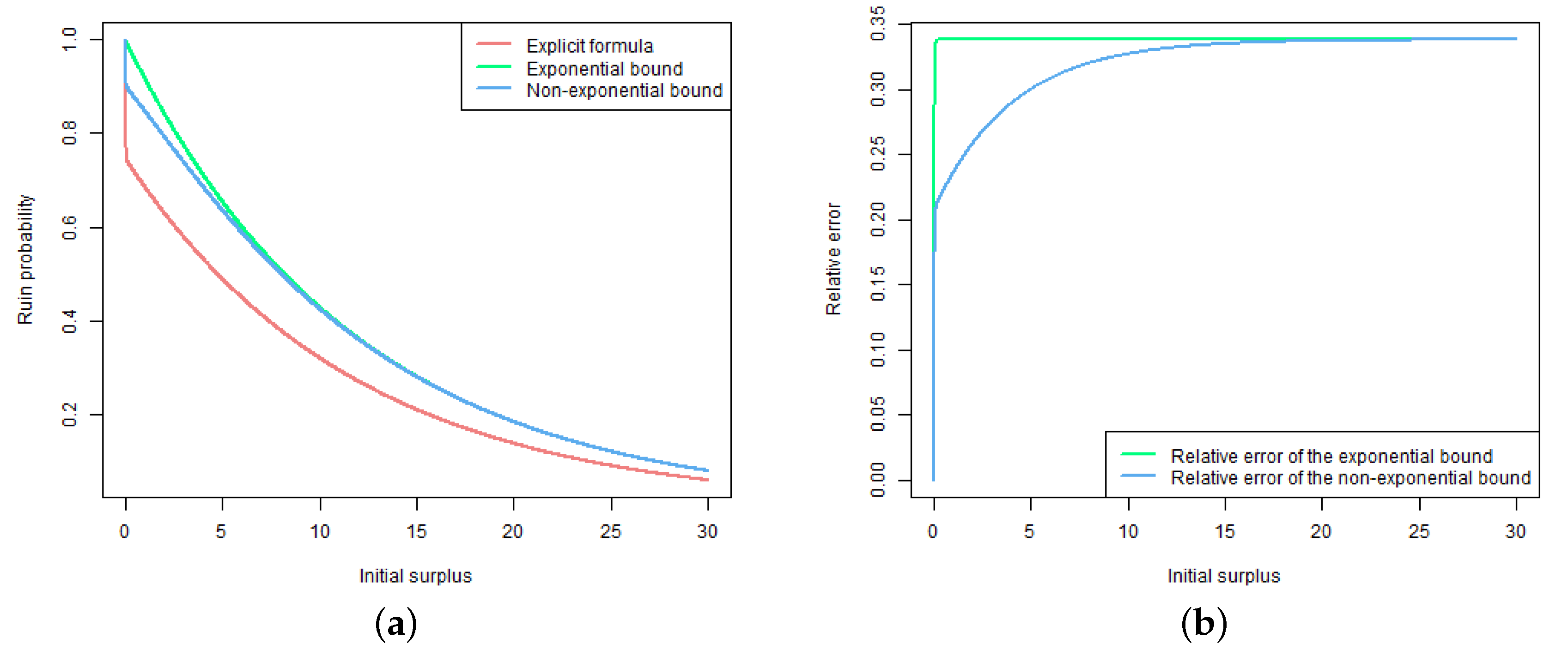
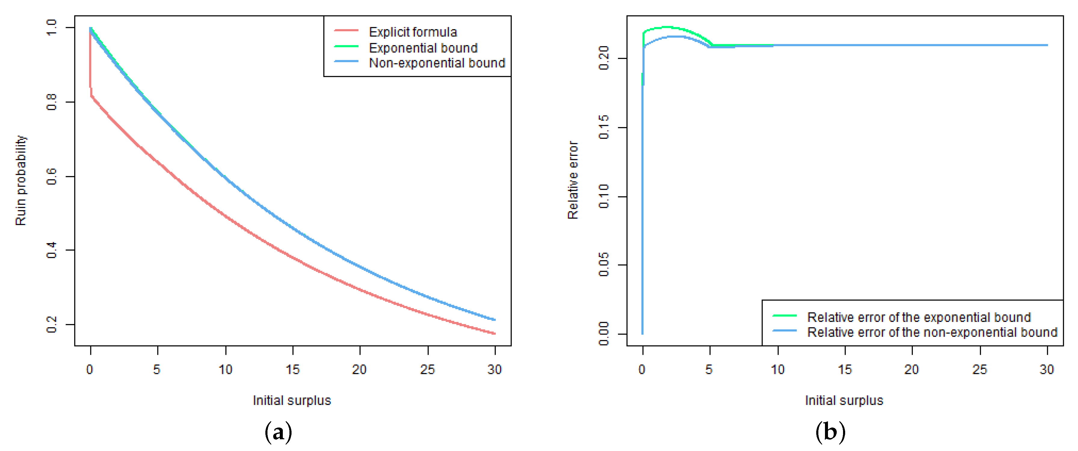
6. Numerical Illustrations

To analyze the results obtained in Section 3, Section 4 and Section 5, we consider a few numerical examples. In all of them, we set $\widehat{\lambda }=2.3$, $\widehat{\mu }=0.2$, $\lambda =0.1$ and $\mu =3$. All calculations are carried out using R software.

Example 1. 

Let $k=1$, i.e., we consider the model with a constant dividend strategy, and let $d=0.05$. We suppose that the premium and claim sizes are exponentially distributed with means $\widehat{\mu }=0.2$ and $\mu =3$.

By Theorems 3 and 4, we get ${\psi }_{\exp }\left(x\right)=e^{-0.08478126x}$ for all $x⩾0$, and we use Proposition 2 to calculate ${\psi }_{\mathrm{non}-\exp }\left(x\right)$. Moreover, by [62] (Theorem 2), we obtain

$$\psi \left(x\right)=0.747121e^{-0.084781x}+0.252879e^{-43.248552x},x⩾0.$$

Note that the exponent in the expression for ${\psi }_{\exp }\left(x\right)$ coincides with one of the exponents in the exact formula for $\psi \left(x\right)$. The results of computations are presented in

Table 1. Results of computations for the model considered in Example 1.

x	$\mathit{\psi }\left(\mathit{x}\right)$	${\mathit{\psi }}_{\mathbf{exp}}\left(\mathit{x}\right)$	$\frac{{\mathit{\psi }}_{\mathbf{exp}}\left(\mathit{x}\right)}{\mathit{\psi }\left(\mathit{x}\right)}-1$	${\mathit{\psi }}_{\mathbf{non}-\mathbf{exp}}\left(\mathit{x}\right)$	$\frac{{\mathit{\psi }}_{\mathbf{non}-\mathbf{exp}}\left(\mathit{x}\right)}{\mathit{\psi }\left(\mathit{x}\right)}-1$
0.2	0.734604	0.983187	0.3384	0.891300	0.2133
0.3	0.728359	0.974886	0.3385	0.886006	0.2164
0.7	0.704072	0.942380	0.3385	0.864594	0.2280
1	0.686390	0.918713	0.3385	0.848330	0.2359
2	0.630595	0.844034	0.3385	0.793602	0.2585
3	0.579336	0.775425	0.3385	0.739289	0.2761
5	0.488980	0.654485	0.3385	0.635932	0.3005
7	0.412715	0.552408	0.3385	0.542882	0.3154
10	0.320030	0.428351	0.3385	0.424847	0.3275
15	0.209455	0.280349	0.3385	0.279687	0.3353
20	0.137085	0.183485	0.3385	0.183359	0.3376
30	0.058721	0.078596	0.3385	0.078591	0.3384
50	0.010774	0.014421	0.3385	0.014421	0.3385
70	0.001977	0.002646	0.3385	0.002646	0.3385

for some values of x.

From Table 1 we conclude that the relative errors ${\psi }_{\exp }\left(x\right)/\psi \left(x\right)-1$ are approximately equal for all values of x, which is also easily seen if we compare formulas for ${\psi }_{\exp }\left(x\right)$ and $\psi \left(x\right)$. Moreover, in this case, the non-exponential bound ${\psi }_{\mathrm{non}-\exp }\left(x\right)$ turns out to be much tighter when the initial surplus is not so large and is becoming closer to ${\psi }_{\exp }\left(x\right)$ with increasing x (see also Figure 1).

Example 2. 

Let $k=2$, $b_1=5$, $d_1=0.05$ and $d_2=0.1$, and let the premium and claim sizes be exponentially distributed with means $\widehat{\mu }=0.2$ and $\mu =3$.

By Theorems 3 and 4, we get ${\psi }_{\exp }\left(x\right)=e^{-0.05186327x}$ for all $x⩾0$, and Theorem 8 and Remark 2 enable us to calculate ${\psi }_{\mathrm{non}-\exp }\left(x\right)$. Explicit formulas are found in [36] (Theorem 3 and Remark 6). Thus, we have

$$\psi \left(x\right)=0.530821e^{-0.084781x}+0.179668e^{-43.248552x}+0.289512,x\in [0,5],$$

$$\psi \left(x\right)=0.826718e^{-0.051863x}-7.043723·{10}^{38}{e}^{-19.28147x},x\in [5,\infty ).$$

We can notice that the exponent in the expression for ${\psi }_{\exp }\left(x\right)$ coincides with one of the exponents in the exact formula for $\psi \left(x\right)$ for $x⩾5$. The results of computations are given in

Table 2. Results of computations for the model considered in Example 2.

x	$\mathit{\psi }\left(\mathit{x}\right)$	${\mathit{\psi }}_{\mathbf{exp}}\left(\mathit{x}\right)$	$\frac{{\mathit{\psi }}_{\mathbf{exp}}\left(\mathit{x}\right)}{\mathit{\psi }\left(\mathit{x}\right)}-1$	${\mathit{\psi }}_{\mathbf{non}-\mathbf{exp}}\left(\mathit{x}\right)$	$\frac{{\mathit{\psi }}_{\mathbf{non}-\mathbf{exp}}\left(\mathit{x}\right)}{\mathit{\psi }\left(\mathit{x}\right)}-1$
0.2	0.811439	0.989681	0.2197	0.981379	0.2094
0.3	0.807002	0.984561	0.2200	0.976501	0.2100
0.7	0.789746	0.964347	0.2211	0.957182	0.2120
1	0.777184	0.949459	0.2217	0.942892	0.2132
2	0.737542	0.901472	0.2223	0.896528	0.2156
3	0.701123	0.855910	0.2208	0.852140	0.2154
5	0.636926	0.771579	0.2114	0.769284	0.2078
7	0.575029	0.695557	0.2096	0.694802	0.2083
10	0.492173	0.595334	0.2096	0.595056	0.2090
15	0.379750	0.459347	0.2096	0.459295	0.2095
20	0.293007	0.354423	0.2096	0.354413	0.2096
30	0.174437	0.211000	0.2096	0.211000	0.2096
50	0.061825	0.074783	0.2096	0.074783	0.2096
70	0.021912	0.026505	0.2096	0.026505	0.2096

for some values of x.

From Table 2 we see that the difference between the relative errors ${\psi }_{\exp }\left(x\right)/\psi \left(x\right)-1$ and ${\psi }_{\mathrm{non}-\exp }\left(x\right)/\psi \left(x\right)-1$ is not so significant as in Example 1 and also vanishes with increasing x (see also Figure 2). This can be explained, in particular, by the fact that to calculate ${\psi }_{\mathrm{non}-\exp }\left(x\right)$, we use Proposition 2 in Example 1 and Theorem 8 together with Remark 2 in Example 2.

Example 3. 

Let now the conditions of Example 2 hold with the difference that $d_1=0.1$ and $d_2=0.05$.

In this case, the exponential bound is the same as that given in Example 2, and ${\psi }_{\mathrm{non}-\exp }\left(x\right)$ is also calculated using Theorem 8 and Remark 2. By [36] (Theorem 3 and Remark 6), we have

$$\psi \left(x\right)=1.204304e^{-0.051863x}+0.218067e^{-19.28147x}-0.422371,x\in [0,5],$$

$$\psi \left(x\right)=0.077253e^{-0.084781x}+1.012903·{10}^{91}{e}^{-43.248552x},x\in [5,\infty ),$$

and the results of computations are presented in

Table 3. Results of computations for the model considered in Example 3.

x	$\mathit{\psi }\left(\mathit{x}\right)$	${\mathit{\psi }}_{\mathbf{exp}}\left(\mathit{x}\right)$	$\frac{{\mathit{\psi }}_{\mathbf{exp}}\left(\mathit{x}\right)}{\mathit{\psi }\left(\mathit{x}\right)}-1$	${\mathit{\psi }}_{\mathbf{non}-\mathbf{exp}}\left(\mathit{x}\right)$	$\frac{{\mathit{\psi }}_{\mathbf{non}-\mathbf{exp}}\left(\mathit{x}\right)}{\mathit{\psi }\left(\mathit{x}\right)}-1$
0.2	0.774117	0.989681	0.2785	0.982463	0.2691
0.3	0.764011	0.984561	0.2887	0.977524	0.2795
0.7	0.738996	0.964347	0.3050	0.958183	0.2966
1	0.721066	0.949459	0.3167	0.943881	0.3090
2	0.663275	0.901472	0.3591	0.897475	0.3531
3	0.608405	0.855910	0.4068	0.853047	0.4021
5	0.506845	0.771579	0.5223	0.770109	0.5194
7	0.426750	0.695557	0.6299	0.694055	0.6264
10	0.330912	0.595334	0.7991	0.594414	0.7963
15	0.216577	0.459347	1.1209	0.458798	1.1184
20	0.141747	0.354423	1.5004	0.354029	1.4976
30	0.060717	0.210100	2.4751	0.210771	2.4714
50	0.011141	0.074783	5.7126	0.074702	5.7054
70	0.002044	0.026505	11.9662	0.026476	11.9522

.

In this case, the exponent in the expression for ${\psi }_{\exp }\left(x\right)$ coincides with one of the exponents in the exact formula for $\psi \left(x\right)$ for $x\in [0,5]$. From Table 3 we deduce that the difference between the relative errors ${\psi }_{\exp }\left(x\right)/\psi \left(x\right)-1$ and ${\psi }_{\mathrm{non}-\exp }\left(x\right)/\psi \left(x\right)-1$ is also not significant and vanishes with increasing x (see also Figure 3). In contrast to Example 2, in this case, the relative errors of both the exponential and non-exponential bounds are acceptable for relatively small values of the initial surplus and are becoming extremely large with increasing x. This follows immediately from the fact that we use only the value of $d_{\max }$ to get the exponential bound, but dividends are actually paid with intensity $d_{\max }$ only when $x\in [0,5]$.

Example 4. 

Let $k=1$ and $d=0.05$. We suppose that the premium sizes are exponentially distributed with mean $\widehat{\mu }=0.2$, and claim sizes have the hyperexponential distribution described in Section 3.3 with $n=3$, $p_1=0.1$, $p_2=0.4$, $p_3=0.5$, ${\mu }_1=1$, ${\mu }_2=2.7$ and ${\mu }_3=3.64$.

By Theorems 3 and 5, we get ${\psi }_{\exp }\left(x\right)=e^{-0.07859704x}$ for all $x⩾0$ since $R=0.07859704$ is the only root of (13) on $(0,1/3.64)$. To calculate ${\psi }_{\mathrm{non}-\exp }\left(x\right)$, we apply Proposition 3. In addition, by Theorem 9, we get

$$\psi \left(x\right)=0.736579e^{-0.078597x}+0.006399e^{-0.336382x}+0.004177e^{-0.978789x}+0.252845e^{-43.251328x},x⩾0,$$

and the results of computations are presented in

Table 4. Results of computations for the model considered in Example 4.

x	$\mathit{\psi }\left(\mathit{x}\right)$	${\mathit{\psi }}_{\mathbf{exp}}\left(\mathit{x}\right)$	$\frac{{\mathit{\psi }}_{\mathbf{exp}}\left(\mathit{x}\right)}{\mathit{\psi }\left(\mathit{x}\right)}-1$	${\mathit{\psi }}_{\mathbf{non}-\mathbf{exp}}\left(\mathit{x}\right)$	$\frac{{\mathit{\psi }}_{\mathbf{non}-\mathbf{exp}}\left(\mathit{x}\right)}{\mathit{\psi }\left(\mathit{x}\right)}-1$
0.2	0.734553	0.984403	0.3401	0.894135	0.2173
0.3	0.728314	0.976697	0.3410	0.889691	0.2216
0.7	0.704311	0.946468	0.3438	0.871147	0.2369
1	0.687044	0.924412	0.3455	0.856609	0.2468
2	0.633290	0.854538	0.3494	0.806126	0.2729
3	0.584412	0.789946	0.3517	0.754893	0.2917
5	0.498441	0.675039	0.3543	0.656260	0.3166
7	0.425505	0.576846	0.3557	0.566634	0.3317
10	0.335864	0.455677	0.3567	0.451513	0.3443
15	0.226613	0.307600	0.3574	0.306636	0.3531
20	0.152952	0.207642	0.3576	0.207412	0.3561
30	0.069694	0.094618	0.3576	0.094604	0.3574
50	0.014471	0.019647	0.3576	0.019647	0.3576
70	0.003005	0.004079	0.3576	0.004079	0.3576

.

We can notice again that the exponent in the expression for ${\psi }_{\exp }\left(x\right)$ coincides with one of the exponents in the exact formula for $\psi \left(x\right)$. As in Example 1, ${\psi }_{\mathrm{non}-\exp }\left(x\right)$ is much tighter than ${\psi }_{\exp }\left(x\right)$ for relatively small values of the initial surplus and is becoming closer to it with increasing x (see also Figure 4).

Example 5. 

Let $k=1$ and $d=0.05$. We suppose that the premium and claim sizes have the Erlang distributions described in Section 3.4 with $\widehat{n}=2$, $\widehat{\beta }=0.1$, $n=2$ and $\beta =1.5$.

In this case, $R=0.1165578$ is the only root of (17) on $(0,1/1.5)$. Hence, Theorems 3 and 6 give that ${\psi }_{\exp }\left(x\right)=e^{-0.1165578x}$ for all $x⩾0$. To calculate ${\psi }_{\mathrm{non}-\exp }\left(x\right)$, we apply Proposition 4. In addition, by Theorem 10, we get

$$\psi \left(x\right)=0.77443e^{-0.116558x}-0.030942e^{-0.983004x}+0.256513e^{-46.561732x},x⩾0,$$

and the results of computations are presented in

Table 5. Results of computations for the model considered in Example 5.

x	$\mathit{\psi }\left(\mathit{x}\right)$	${\mathit{\psi }}_{\mathbf{exp}}\left(\mathit{x}\right)$	$\frac{{\mathit{\psi }}_{\mathbf{exp}}\left(\mathit{x}\right)}{\mathit{\psi }\left(\mathit{x}\right)}-1$	${\mathit{\psi }}_{\mathbf{non}-\mathbf{exp}}\left(\mathit{x}\right)$	$\frac{{\mathit{\psi }}_{\mathbf{non}-\mathbf{exp}}\left(\mathit{x}\right)}{\mathit{\psi }\left(\mathit{x}\right)}-1$
0.2	0.731189	0.976958	0.3361	0.958695	0.3111
0.3	0.724778	0.965637	0.3323	0.948061	0.3081
0.7	0.698203	0.921649	0.3200	0.906691	0.2986
1	0.677648	0.889979	0.3133	0.876812	0.2939
2	0.609064	0.792062	0.3005	0.783729	0.2868
3	0.544288	0.704918	0.2951	0.699832	0.2858
5	0.432167	0.558339	0.2920	0.556572	0.2879
7	0.342451	0.442239	0.2914	0.441661	0.2897
10	0.241421	0.311742	0.2913	0.311641	0.2909
15	0.134796	0.174058	0.2913	0.174053	0.2912
20	0.075262	0.097183	0.2913	0.097183	0.2913
30	0.023462	0.030296	0.2913	0.030296	0.2913
50	0.002280	0.002944	0.2913	0.002944	0.2913
70	0.000222	0.000286	0.2913	0.000286	0.2913

.

Here, we can also see that the exponent in the expression for ${\psi }_{\exp }\left(x\right)$ coincides with one of the exponents in the exact formula for $\psi \left(x\right)$, and ${\psi }_{\mathrm{non}-\exp }\left(x\right)$ is becoming closer to ${\psi }_{\exp }\left(x\right)$ with increasing x. In contrast to Examples 1 and 4, ${\psi }_{\mathrm{non}-\exp }\left(x\right)$ is not much tighter than ${\psi }_{\exp }\left(x\right)$ for relatively small values of the initial surplus (see also Figure 5).

7. Conclusions

In this article, we obtained an exponential bound for the ruin probability in the risk model with stochastic premiums and a multi-layer dividend strategy and investigated conditions, under which it holds for the exponential, hyperexponential and Erlang distributions of the premium and claim sizes. Using this exponential bound we constructed non-exponential upper bounds, which turn out to be tighter in a number of cases. Moreover, we derived explicit formulas for the ruin probability when the premium and claim sizes have either the hyperexponential or the Erlang distributions and used the formulas to investigate how tight the bounds are.

On the basis of the numerical examples considered above, we can make the following conclusions. First of all, in all the examples considered above, the exponent in the expression for ${\psi }_{\exp }\left(x\right)$ coincides with one of the exponents in the exact formula for $\psi \left(x\right)$.

Next, if $k=1$, which implies a constant dividend strategy, then the relative errors of the exponential bound are acceptable. If the premium and claim sizes have the exponential and hyperexponential distributions, ${\psi }_{\mathrm{non}-\exp }\left(x\right)$ is much tighter than ${\psi }_{\exp }\left(x\right)$ when the initial surplus is not so large, whereas this difference is not so significant if the premium and claim sizes have the Erlang distributions with $\widehat{n}=2$ and $n=2$. Moreover, ${\psi }_{\mathrm{non}-\exp }\left(x\right)$ is becoming closer to ${\psi }_{\exp }\left(x\right)$ with increasing x.

If $k=2$, then the results are acceptable provided that $d_2=d_{\max }$. If $d_1=d_{\max }$, the relative errors of both the exponential and non-exponential bounds are acceptable for relatively small values of the initial surplus and are becoming extremely large with increasing x. In addition, if $k=2$, the difference between the relative errors ${\psi }_{\exp }\left(x\right)/\psi \left(x\right)-1$ and ${\psi }_{\mathrm{non}-\exp }\left(x\right)/\psi \left(x\right)-1$ is not so significant, although ${\psi }_{\mathrm{non}-\exp }\left(x\right)$ is still somewhat tighter. This can be explained, in particular, by the fact that we use Theorem 8 and Remark 2 to calculate ${\psi }_{\mathrm{non}-\exp }\left(x\right)$ in this case, whereas Propositions 2–4 are applied to this end if $k=1$.

Finally, from all the examples considered above, we conclude that when the relative errors of the exponential bound are large, so are the relative errors of the non-exponential bound because it is constructed using the exponential one.

References

1. Grandell, J. Aspects of Risk Theory; Springer: New York, NY, USA, 1991. [Google Scholar]
2. Rolski, T.; Schmidli, H.; Schmidt, V.; Teugels, J. Stochastic Processes for Insurance and Finance; John Wiley & Sons: Chichester, UK, 1999. [Google Scholar]
3. Asmussen, S.; Albrecher, H. Ruin Probabilities; World Scientific: Singapore, 2010. [Google Scholar]
4. Mishura, Y.; Ragulina, O. Ruin Probabilities: Smoothness, Bounds, Supermartingale Approach; ISTE Press—Elsevier: London, UK, 2016. [Google Scholar]
5. Schmidli, H. Risk Theory; Springer: Cham, Switzerland, 2018. [Google Scholar]
6. Schmidli, H. Stochastic Control in Insurance; Springer: London, UK, 2008. [Google Scholar]
7. Gerber, H.U.; Shiu, E.S.W. On the time value of ruin. N. Am. Actuar. J. 1998, 2, 48–72. [Google Scholar] [CrossRef]
8. Chadjiconstantinidis, S.; Vrontos, S. On a renewal risk process with dependence under a Farlie–Gumbel– Morgenstern copula. Scand. Actuar. J. 2014, 2014, 125–158. [Google Scholar] [CrossRef] [Green Version]
9. Cheng, Y.; Tang, Q. Moments of the surplus before ruin and the deficit of ruin in the Erlang(2) risk process. N. Am. Actuar. J. 2003, 7, 1–12. [Google Scholar] [CrossRef]
10. Cossette, H.; Marceau, E.; Marri, F. On the compound Poisson risk model with dependence based on a generalized Farlie–Gumbel–Morgenstern copula. Insur. Math. Econ. 2008, 43, 444–455. [Google Scholar] [CrossRef]
11. Cossette, H.; Marceau, E.; Marri, F. Analysis of ruin measures for the classical compound Poisson risk model with dependence. Scand. Actuar. J. 2010, 2010, 221–245. [Google Scholar] [CrossRef]
12. Gerber, H.U.; Shiu, E.S.W. The time value of ruin in a Sparre Andersen model. N. Am. Actuar. J. 2005, 9, 49–69. [Google Scholar] [CrossRef]
13. Navickienė, O.; Sprindys, J.; Šiaulys, J. The Gerber–Shiu discounted penalty function for the bi-seasonal discrete time risk model. Informatica 2018, 29, 733–756. [Google Scholar] [CrossRef] [Green Version]
14. Sun, L.-J. The expected discounted penalty at ruin in the Erlang(2) risk process. Stat. Probab. Lett. 2005, 72, 205–217. [Google Scholar] [CrossRef]
15. De Finetti, B. Su un’impostazione alternativa dell teoria colletiva del rischio. Trans. XV Int. Congr. Actuar. 1957, 2, 433–443. [Google Scholar]
16. Li, S.; Garrido, J. On a class of renewal risk models with a constant dividend barrier. Insur. Math. Econ. 2004, 35, 691–701. [Google Scholar] [CrossRef]
17. Lin, X.S.; Pavlova, K.P. The compound Poisson risk model with a threshold dividend strategy. Insur. Math. Econ. 2006, 38, 57–80. [Google Scholar] [CrossRef]
18. Landriault, D. Constant dividend barrier in a risk model with interclaim-dependent claim sizes. Insur. Math. Econ. 2008, 42, 31–38. [Google Scholar] [CrossRef]
19. Li, B.; Wu, R.; Song, M. A renewal jump-diffusion process with threshold dividend strategy. J. Comput. Appl. Math. 2009, 228, 41–55. [Google Scholar] [CrossRef] [Green Version]
20. Chi, Y.; Lin, X.S. On the threshold dividend strategy for a generalized jump-diffusion risk model. Insur. Math. Econ. 2011, 48, 326–337. [Google Scholar] [CrossRef]
21. Shi, Y.; Liu, P.; Zhang, C. On the compound Poisson risk model with dependence and a threshold dividend strategy. Stat. Probab. Lett. 2013, 83, 1998–2006. [Google Scholar] [CrossRef]
22. Cossette, H.; Marceau, E.; Marri, F. On a compound Poisson risk model with dependence and in the presence of a constant dividend barrier. Appl. Stoch. Models Bus. Ind. 2014, 30, 82–98. [Google Scholar] [CrossRef]
23. Wang, W. The perturbed Sparre Andersen model with interest and a threshold dividend strategy. Methodol. Comput. Appl. Probab. 2015, 17, 251–283. [Google Scholar] [CrossRef]
24. Ragulina, O. The risk model with stochastic premiums, dependence and a threshold dividend strategy. Mod. Stoch. Theory Appl. 2017, 4, 315–351. [Google Scholar] [CrossRef] [Green Version]
25. Albrecher, H.; Hartinger, J. A risk model with multilayer dividend strategy. N. Am. Actuar. J. 2007, 11, 43–64. [Google Scholar] [CrossRef]
26. Badescu, A.; Drekic, S.; Landriault, D. On the analysis of a multi-threshold Markovian risk model. Scand. Actuar. J. 2007, 2007, 248–260. [Google Scholar] [CrossRef]
27. Lin, X.S.; Sendova, K.P. The compound Poisson risk model with multiple thresholds. Insur. Math. Econ. 2008, 42, 617–627. [Google Scholar] [CrossRef]
28. Badescu, A.; Landriault, D. Recursive calculation of the dividend moments in a multi-threshold risk model. N. Am. Actuar. J. 2008, 12, 74–88. [Google Scholar] [CrossRef]
29. Yang, H.; Zhang, Z. Gerber–Shiu discounted penalty function in a Sparre Andersen model with multi-layer dividend strategy. Insur. Math. Econ. 2008, 42, 984–991. [Google Scholar] [CrossRef]
30. Yang, H.; Zhang, Z. The perturbed compound Poisson risk model with multi-layer dividend strategy. Stat. Probab. Lett. 2009, 79, 70–78. [Google Scholar] [CrossRef]
31. Mitric, I.-R.; Sendova, K.P.; Tsai, C.C.-L. On a multi-threshold compound Poisson process perturbed by diffusion. Stat. Probab. Lett. 2010, 80, 366–375. [Google Scholar] [CrossRef]
32. Deng, C.; Zhou, J.; Deng, Y. The Gerber–Shiu discounted penalty function in a delayed renewal risk model with multi-layer dividend strategy. Stat. Probab. Lett. 2012, 82, 1648–1656. [Google Scholar] [CrossRef]
33. Jiang, W.; Yang, Z.; Li, X. The discounted penalty function with multi-layer dividend strategy in the phase-type risk model. Stat. Probab. Lett. 2012, 82, 1358–1366. [Google Scholar] [CrossRef]
34. Zhou, Z.; Xiao, H.; Deng, Y. Markov-dependent risk model with multi-layer dividend strategy. Appl. Math. Comput. 2015, 252, 273–286. [Google Scholar] [CrossRef]
35. Xie, J.-H.; Zou, W. On the expected discounted penalty function for a risk model with dependence under a multi-layer dividend strategy. Comm. Stat. Theory Methods 2017, 46, 1898–1915. [Google Scholar] [CrossRef]
36. Ragulina, O. The risk model with stochastic premiums and a multi-layer dividend strategy. Mod. Stoch. Theory Appl. 2019, 6, 285–309. [Google Scholar] [CrossRef]
37. Albrecher, H.; Constantinescu, C.; Loisel, S. Explicit ruin formulas for models with dependence among risks. Insur. Math. Econ. 2011, 48, 265–270. [Google Scholar] [CrossRef] [Green Version]
38. Constantinescu, C.; Samorodnitsky, G.; Zhu, W. Ruin probabilities in classical risk models with gamma claims. Scand. Actuar. J. 2018, 2018, 555–575. [Google Scholar] [CrossRef]
39. Dufresne, F.; Gerber, H.U. Three methods to calculate the probability of ruin. ASTIN Bull. 1989, 19, 71–90. [Google Scholar] [CrossRef] [Green Version]
40. Gómez-Déniz, E.; Sarabia, J.M.; Calderín-Ojeda, E. Ruin probability functions and severity of ruin as a statistical decision problem. Risks 2019, 7, 68. [Google Scholar] [CrossRef] [Green Version]
41. Ramsay, C.M. A solution to the ruin problem for Pareto distributions. Insur. Math. Econ. 2003, 33, 109–116. [Google Scholar] [CrossRef]
42. Mishura, Y.S.; Ragulina, O.Y.; Stroev, O.M. Analytic property of infinite-horizon survival probability in a risk model with additional funds. Theory Probab. Math. Stat. 2015, 91, 131–143. [Google Scholar] [CrossRef]
43. Thorin, O. The ruin problem in case the tail of the claim distribution is completely monotone. Scand. Actuar. J. 1973, 1973, 100–119. [Google Scholar] [CrossRef]
44. Navickienė, O.; Sprindys, J.; Šiaulys, J. Ruin probability for the bi-seasonal discrete time risk model with dependent claims. Mod. Stoch. Theory Appl. 2019, 6, 133–144. [Google Scholar] [CrossRef] [Green Version]
45. Grigutis, A.; Šiaulys, J. Ultimate time survival probability in three-risk discrete time risk model. Mathematics 2020, 8, 147. [Google Scholar] [CrossRef] [Green Version]
46. Gerber, H.U. Martingales in risk theory. Z. Mitt. Ver. Schweiz. 1973, 73, 205–216. [Google Scholar]
47. Boikov, A.V. The Cramér–Lundberg model with stochastic premium process. Theory Probab. Appl. 2003, 47, 489–493. [Google Scholar] [CrossRef]
48. Yang, H.; Zhang, L. Martingale method for ruin probability in an autoregressive model with constant interest rate. Probab. Eng. Inf. Sci. 2003, 17, 183–198. [Google Scholar] [CrossRef] [Green Version]
49. Grandell, J.; Schmidli, H. Ruin probabilities in a diffusion enviroment. J. Appl. Probab. 2011, 48A, 39–50. [Google Scholar] [CrossRef]
50. Mishura, Y.; Ragulina, O.; Stroev, O. Practical approaches to the estimation of the ruin probability in a risk model with additional funds. Mod. Stoch. Theory Appl. 2014, 1, 167–180. [Google Scholar] [CrossRef] [Green Version]
51. Mishura, Y.; Perestyuk, M.; Ragulina, O. Ruin probability in a risk model with variable premium intensity and risky investments. Opusc. Math. 2015, 35, 333–352. [Google Scholar] [CrossRef]
52. Kievinaitě, D.; Šiaulys, J. Exponential bounds for the tail probability of the supremum of an inhomogeneous random walk. Mod. Stoch. Theory Appl. 2018, 5, 129–143. [Google Scholar] [CrossRef] [Green Version]
53. Kizineviě, E.; Šiaulys, J. The exponential estimate of the ultimate ruin probability for the non-homogeneous renewal risk model. Risks 2018, 6, 20. [Google Scholar] [CrossRef] [Green Version]
54. Andrulytė, I.M.; Bernackaitė, E.; Kievinaitė, D.; Šiaulys, J. A Lundberg-type inequality for an inhomogeneous renewal risk model. Mod. Stoch. Theory Appl. 2015, 2, 173–184. [Google Scholar] [CrossRef] [Green Version]
55. Yang, H. Non-exponential bounds for ruin probability with interest effect included. Scand. Actuar. J. 1999, 1999, 66–79. [Google Scholar] [CrossRef]
56. Embrechts, P.; Villasenor, J.A. Ruin estimates for large claims. Insur. Math. Econ. 1988, 7, 269–274. [Google Scholar] [CrossRef]
57. De Vylder, F.; Goovaerts, M. Bounds for classical ruin probabilities. Insur. Math. Econ. 1984, 3, 121–131. [Google Scholar] [CrossRef]
58. Sundt, B.; Teugels, J. Ruin estimates under interest force. Insur. Math. Econ. 1995, 16, 7–22. [Google Scholar] [CrossRef]
59. Cai, J.; Garrido, J. Two-sided bounds for ruin probabilities when the adjustment coefficient does not exist. Scand. Actuar. J. 1999, 1999, 80–92. [Google Scholar] [CrossRef]
60. Kalashnikov, V. Bounds for ruin probabilities in the presence of large claims and their comparison. N. Am. Actuar. J. 1999, 3, 116–128. [Google Scholar] [CrossRef]
61. Konstantinides, D.; Tang, Q.; Tsitsiashvili, G. Estimates for the ruin probability in the classical risk model with constant interest force in the presence of heavy tails. Insur. Math. Econ. 2002, 31, 447–460. [Google Scholar] [CrossRef] [Green Version]
62. Ragulina, O. Simple approximations for the ruin probability in the risk model with stochastic premiums and a constant dividend strategy. Mod. Stoch. Theory Appl. 2020, 7, 245–265. [Google Scholar] [CrossRef]
63. Mordecki, E. Ruin probabilities for Lévy processes with mixed-exponential negative jumps. Theory Probab. Appl. 2003, 48, 170–176. [Google Scholar] [CrossRef] [Green Version]
64. Bao, Z. The expected discounted penalty at ruin in the risk process with random income. Appl. Math. Comput. 2006, 179, 559–566. [Google Scholar] [CrossRef]
65. Lewis, A.; Mordecki, E. Wiener-Hopf factorization for Lévy processes having positive jumps with rational transforms. J. Appl. Probab. 2008, 45, 118–134. [Google Scholar] [CrossRef] [Green Version]
66. Yang, H.; Zhang, Z. On a class of renewal risk model with random income. Appl. Stoch. Models Bus. Ind. 2009, 25, 678–695. [Google Scholar] [CrossRef]
67. Labbé, C.; Sendova, K.P. The expected discounted penalty function under a risk model with stochastic income. Appl. Math. Comput. 2009, 215, 1852–1867. [Google Scholar] [CrossRef]
68. Zhang, Z.; Yang, H. A generalized penalty function in the Sparre Andersen risk model with two-sided jumps. Stat. Probab. Lett. 2010, 80, 597–607. [Google Scholar] [CrossRef]
69. Zhao, X.; Yin, C. The Gerber–Shiu expected discounted penalty function for Lévy insurance risk processes. Acta Math. Appl. Sin. 2010, 26, 575–586. [Google Scholar] [CrossRef]
70. Zhao, Y.; Yin, C. The expected discounted penalty function under a renewal risk model with stochastic income. Appl. Math. Comput. 2012, 218, 6144–6154. [Google Scholar] [CrossRef]
71. Xie, J.; Zou, W. On a risk model with random incomes and dependence between claim sizes and claim intervals. Indag. Math. 2013, 24, 557–580. [Google Scholar] [CrossRef]
72. Wang, Y.; Yu, W.; Huang, Y. Estimating the Gerber–Shiu function in a compound Poisson risk model with stochastic premium income. Discret. Dyn. Nat. Soc. 2019, 2019, 5071268. [Google Scholar] [CrossRef]
Figure 1. Comparison of the results for the model considered in Example 1: (a) Ruin probability given by the explicit formula as well as the exponential and non-exponential bounds for it. (b) Relative errors of the exponential and non-exponential bounds.
Mathematics 08 01885 g001
Figure 2. Comparison of the results for the model considered in Example 2: (a) Ruin probability given by the explicit formula as well as the exponential and non-exponential bounds for it. (b) Relative errors of the exponential and non-exponential bounds.
Mathematics 08 01885 g002
Figure 3. Comparison of the results for the model considered in Example 3: (a) Ruin probability given by the explicit formula as well as the exponential and non-exponential bounds for it. (b) Relative errors of the exponential and non-exponential bounds.
Mathematics 08 01885 g003
Figure 4. Comparison of the results for the model considered in Example 4: (a) Ruin probability given by the explicit formula as well as the exponential and non-exponential bounds for it. (b) Relative errors of the exponential and non-exponential bounds.
Mathematics 08 01885 g004
Figure 5. Comparison of the results for the model considered in Example 5: (a) Ruin probability given by the explicit formula as well as the exponential and non-exponential bounds for it. (b) Relative errors of the exponential and non-exponential bounds.
Mathematics 08 01885 g005